FepiM: A Novel Inverse Piecewise Method to Determine Isothermal Flow Curves for Hot Working

Abstract

In forming simulations, flow curves are cardinal inputs to predict features, such as forming forces and material flow. The laboratory-scale experiments to determine them, like compression or tensile tests, are affected by deformation heating, restricting direct flow curve determination. In principle, the current analytical and inverse methods determine flow curves from these tests, but while the analytical methods assume a simplified temperature profile, the inverse methods require a closed-form flow curve equation, which mostly cannot capture complex material behavior like multiple recrystallization cycles. Therefore, the inverse piecewise flow curve determination method “FepiM” previously developed and published by the current authors is extended by introducing a two-step procedure to obtain isothermal flow curves at elevated temperatures and different strain rates. Thereby, the flow curve is represented as tabular data instead of an equation to reproduce complex flow curve shapes while also compensating the effect of inhomogeneous temperature profiles on the flow stress. First, a flow curve at the highest temperature is determined. In the second step, using this first flow curve as a reference, the flow curves at lower temperatures are obtained via interpolation. Flow curves from conventional compression tests for aluminum and copper in the temperature range of 20–500 °C are predicted, and it is shown that these flow curves can reproduce the experimental forces with a maximum deviation of less than 1%. Therefore, the proposed new piecewise method accurately predicts isothermal flow curves for compression tests, and the method could be further extended to highly inhomogeneous methods in the future.

1. Introduction

Precise and reliable flow curves play a vital role in capturing relevant characteristics, like forming force, material flow, and internal stresses in metal forming simulations. Generally, laboratory-scale experiments, e.g., compression tests, tensile tests, torsion tests, etc., are conducted to determine these flow curves [1]. Though these experiments are performed under controlled conditions, several aspects like friction, deformation heating, heat transfer, etc., restrict the precision when directly converting experimental data to flow curves [2]. Inverse modeling can be used to overcome these issues as all testing conditions are mimicked via FE simulations. Typically, inverse modeling is based on optimizing the parameters of an analytical flow curve equation to match the measured force-displacement curve. Obviously, the prediction accuracy then depends on the capabilities of the chosen analytical equation. In contrast, inverse flow curve determination can do without analytical equations if a piecewise approach is followed, where the flow curve is constructed sequentially. Currently, these approaches are restricted to determining flow curves from room-temperature tensile tests. The current paper aims to extend the inverse piecewise flow curve determination to elevated temperatures and different strain rates. Conventional compression tests are used here for two main reasons: Firstly, analytical flow stress evaluation concepts are well established for these tests and thus can be used for validation of the novel approach, and secondly compression tests are widespread in hot working of bulk materials due to the prevailing compressive stress states [3]. As lubricated compression tests are rather homogeneous, only moderate accuracy improvements are to be expected. However, once validated, the novel piecewise approach may greatly improve the evaluation accuracy compared to analytical methods for highly inhomogeneous experiments like torsion tests [4] or hot tensile tests [5] beyond necking.

To set the stage, established conventional and inverse flow stress determination approaches are reviewed in the following section with special emphasis on the ability to reproduce inhomogeneity inside the test specimen.

2. State of the Art

In compression tests, inhomogeneity due to friction can be controlled to some extent by lubrication mostly in combination with special sample geometries, e.g., Rastegaev samples with collar to contain a lubricant pit [6]. In contrast, the temperature inhomogeneity due to the conversion of plastic work to heat energy the so-called “deformation heating” is unavoidable. This phenomenon is more prevalent for experiments at lower temperatures and higher strain rates where the material exhibits high flow stress values. Concurrently, experiments at high strain rates do not have ample time to balance this temperature increase through heat transfer to the tool and environment [7]. The temperature of the specimen increases with deformation and deviates from the desired nominal temperature, typically set at the start of the experiment via an isothermal furnace. Since the flow stress of a material is a function of temperature, temperature changes due to deformation heating inevitably influence the measured forces. Thus, the flow curve calculated from experimental data does not correspond to the nominal testing temperature but to an average temperature slightly above that. To instead obtain an isothermal flow curve, the further processing steps described below in detail are indispensable.

These isothermal flow curves are essentially required for finite element (FE) simulations of metal-forming processes as tabular data of a flow curve field, i.e., the flow stress ${\mathsf{\sigma }}_{\mathrm{f}}$ as a function of constant strain $\mathsf{\phi }$, strain rate $\dot{\mathsf{\phi }}$, and temperature $\mathrm{T}$ must be provided [8]. In addition, several micromechanical-based material models identify critical conditions, such as the onset of dynamic recrystallization (DRX), through flow curves at isothermal conditions [9]. The methods to obtain isothermal flow curves documented in the literature can be divided into two categories: analytical and inverse methods. Both are reviewed below for flow curve determination mostly via compression tests.

2.1. Analytical Method for Isothermal Flow Curve Determination

Cylindrical uniaxial compression tests are one of the most commonly used tests to obtain flow curves [3]. The average flow stress ${\mathsf{\sigma }}_{\mathrm{f}}$ and plastic strain ${\mathsf{\phi }}_{\mathrm{measured}}$ from an experiment performed at a nominal testing temperature ${\mathrm{T}}_{\mathrm{testing}}$ and strain rate of ${\dot{\mathsf{\phi }}}_{\mathrm{measured}}$ can be calculated as a function of the displacement of the tool based on actual measurements using [1]:

$${\mathsf{\sigma }}_{\mathrm{f},\mathrm{measured}}=\frac{\mathrm{F}}{\mathrm{A}} \mathrm{and} {\mathsf{\phi }}_{\mathrm{measured}}=\left|\ln \frac{{\mathrm{h}}_0}{{\mathrm{h}}_1}\right|$$

(1)

where F and A are the current force and current cross-sectional area, respectively, and ${\mathrm{h}}_0$ and ${\mathrm{h}}_1$ are the original and current heights of the specimen. However, due to deformation heating, the flow curve obtained via Equation (1) fails to correspond to a constant ${\mathrm{T}}_{\mathrm{testing}}$. The procedure to correct this temperature-induced deviation of the flow stress is referred to as “temperature compensation” [10].

The existing analytical methods achieve this compensation in two steps and they work with tabular data of a flow curve field, i.e., sampled data points of ${\mathsf{\sigma }}_{\mathrm{f},\mathrm{measured}}$, ${\mathsf{\phi }}_{\mathrm{measured}}$ calculated from experiments performed at the nominal testing temperature ${\mathrm{T}}_{\mathrm{testing}}$. At first, the average temperature deviation from ${\mathrm{T}}_{\mathrm{testing}}$ at each data point is calculated. Laasraoui et al. [11] obtain the heat generated during deformation using Equation (2)

$$\mathsf{\Delta }{\mathrm{T}}_{+}= \mathrm{D} \frac{\int {\mathsf{\sigma }}_{\mathrm{f},\mathrm{measured}}\left(\mathsf{\phi }\right){\mathrm{d}\mathsf{\phi }}_{\mathrm{measured}}}{{\mathsf{\rho } \mathrm{c}}_{\mathrm{p}}}$$

(2)

where the term $\int {\mathsf{\sigma }}_{\mathrm{f}} \mathrm{d}\mathsf{\phi }$ corresponds to the area under the measured flow curve at different strain levels, $\mathsf{\rho }$ and ${\mathrm{c}}_{\mathrm{p}}$ are the density and specific heat capacity of the material, respectively. $\mathrm{D} (0<\mathrm{D}<1)$ is the dissipation coefficient that represents the proportion of deformation energy that is converted to heat and typically ranges from 0.9 to 0.95 [11]. In addition to Equation (2), Kopp et al. [10] also consider heat transfer between the specimen and tool, defined by Equation (3)

$$\mathsf{\Delta }{\mathrm{T}}_{-}=-\frac{2\mathsf{\alpha }\mathrm{A}}{{\mathsf{\rho } \mathrm{c}}_{\mathrm{p}} \mathrm{V}} ({\mathrm{T}}_{\mathrm{t}-1}-{\mathrm{T}}_{\mathrm{tool}})\mathsf{\Delta }\mathrm{t}$$

(3)

where $\mathrm{A}$ and $\mathrm{V}$ are the contact area between the specimen and tool and volume of the specimen, respectively, ${\mathrm{T}}_{\mathrm{Die}}$ is the tool temperatures, $\mathsf{\alpha }$ is the interfacial heat transfer coefficient (IHC) between the specimen and tool, ${\mathrm{T}}_{\mathrm{t}-1}$ is the specimen temperature from the last time increment, and $\mathsf{\Delta }\mathrm{t}$ is the timestep size. The heat lost to the environment due to convection and radiation is considered insignificant in comparison and therefore neglected. Using Equations (2) and (3), the net average temperature change ($\mathsf{\Delta }{\mathrm{T}}_{+}+ \mathsf{\Delta }{\mathrm{T}}_{-}$) is calculated. Zhao et al. [7] further proposed to consider the heat generated due to friction, but when using Rastegaev compression test samples, this addition can be ignored [10].

In the second step of temperature compensation, ${\mathrm{T}}_{\mathrm{actual} }({\mathrm{T}}_{\mathrm{testing} }+ \mathsf{\Delta }\mathrm{T}$) is thereafter used to correct the measured flow stress ${\mathsf{\sigma }}_{\mathrm{f},\mathrm{measured}}$ to its corresponding nominal testing temperature. Kopp et al. [10] and Zhao et al. [7] used a similar linear interpolation equation shown below

$${\mathsf{\sigma }}_{\mathrm{f},\mathrm{actual}}={\mathsf{\sigma }}_{\mathrm{f},\mathrm{measured}}+\mathsf{\Delta }\mathrm{T} {\left.\frac{\mathrm{d}{\mathsf{\sigma }}_{\mathrm{f}}}{\mathrm{d}T}\right|}_{\mathsf{\epsilon }.\dot{\mathsf{\epsilon }}}.$$

(4)

By plotting data of ${\mathsf{\sigma }}_{\mathrm{f},\mathrm{measured}}$ with respect to ${\mathrm{T}}_{\mathrm{actual}}$ and according to ${\mathrm{T}}_{\mathrm{actual}}$ and $\mathsf{\Delta }\mathrm{T}$, the two nearest sampled data points on the plot are obtained to calculate the derivative of flow stress with respect to temperature. Using this derivative in Equation (4), the desired actual flow stress value corresponding to ${\mathrm{T}}_{\mathrm{actual}}$ can be obtained.

Alternatively, Xiong et al. [12] proposed to fit the array of data points ${\mathsf{\sigma }}_{\mathrm{f},\mathrm{measured}}$, ${\mathsf{\phi }}_{\mathrm{measured}}$ and ${\mathrm{T}}_{\mathrm{actual}}$ at a constant strain rate to a thin plate spline (TPS) surface. Then, desired isothermal flow curves at constant ${\mathrm{T}}_{\mathrm{testing}}$ are extracted from the fit. This concept eliminated undesirable kinks that appear in the isothermal flow curves determined from Equation (4), especially for high-strength materials.

Though the above two-step analytical methods derive isothermal flow curves from experimental data, this offline approach fails to consider the inhomogeneity that occur during experiments. For example, although temperature inhomogeneity is expected due to heat transfer between the specimen and tool as well as to the environment, Equation (2) describes temperature raise as an average quantity by only considering the global flow stress and plastic strain values. Similarly, the flow stress calculation in Equation (1) cannot describe the average flow stress after the onset of bulging [13].

2.2. Inverse Methods for Isothermal Flow Curve Determination

Equation based methods: To overcome the challenges posed by inhomogeneity inside the specimen, online temperature compensation methods based on inverse modeling were developed where the flow curve is represented by empirical constitutive functions. Therefore, an FE model of the experiments is used, to iteratively determine the unknown parameters in the chosen empirical equation such that the error between the simulated and experimental forces is minimized. Isothermal flow curves are then extracted from the optimized constitutive function. Simulations inherently address deformation heating and other heat transfer mechanisms, and hence, the additional steps discussed above are not required. Forestier et al. [14] performed 3D coupled thermomechanical compression test simulations to inversely identity the parameters of the Norton–Hoff constitutive law. Cao et al. [15] recently determined flow curves beyond necking from tensile test experiments by optimizing parameters of a modified Swift constitutive law. However, the accuracy of these models highly depends on the a priori chosen constitutive model [5]. In addition, flow curve description for materials exhibiting complex flow behavior like multiple dynamic recrystallization cycles cannot typically be captured by these models.

Piecewise methods: Alternatively, inverse piecewise flow curve determination methods were introduced. Instead of fitting a constitutive model, here, the flow curve is determined in a piecewise manner by minimizing the deviation between the simulated and experimental forces at different displacements points sequentially. As mentioned earlier the flow curve determination becomes independent of any constitutive equation. The IFD (inverse FE procedure based on digital image correlation) concept by Kamaya et al. [16] is illustrated in Figure 1, where experimental force versus axial strain in the necking region is determined and sampled at different strain levels. The strain in the necking proportion is measured using digital image correlation (DIC). As shown in Figure 1, the tensile test FE simulation is performed until the strain in the necking zone reaches the sampled strain ${\mathsf{\phi }}_{\mathrm{i}}$ measured in experiments, and an arbitrary flow stress ${\mathsf{\sigma }}_{\mathrm{i}}$ is assigned to the measured strain. Then, by iteratively performing simulations, ${\mathsf{\sigma }}_{\mathrm{i}}$ is optimized such that the error between the experimental and simulated forces is minimized. This is repeated at different strains. Zhao et al. [17] also developed a similar approach to predict the flow curves in tensile tests beyond necking and used analytical methods to obtain the experimental force versus axial strain curve. Therefore, these proposed methods require local strain information in the necking zone, and approximations based on analytical equations or additional experimental measurement techniques like DIC are used to obtain this data. At the same time, these flow curves were determined at room temperature and a quasistatic strain rate where the temperature rise due to deformation heating is compensated by heat transfer to the tool and also by convection and radiation [7].

2.3. Assessment of the Literature and Problem Statement

The analytical methods described ignore the thermal inhomogeneity during flow curve evaluation. In contrast, the conventional inverse methods capture the inhomogeneity through simulation models, but their accuracy is highly dependent on the chosen constitutive equation. Although piecewise inverse methods overcome this additional limitation, they are currently restricted to determine flow curves at room temperature and quasistatic rate conditions where a homogenous temperature profile in the specimen can be assumed. Moreover, the existing inverse piecewise methods are restricted to tensile tests and have limited extendibility to bulk material-testing methods when the strain in the specimen is inhomogeneous, e.g., torsion tests or unlubricated compression tests. In these cases, the maximum strain is generally found inside the bulk specimen, and DIC is thus not applicable.

To overcome all limitations mentioned, an inverse piecewise flow curve determination approach “flow curve determination through explicit piecewise inverse modeling (FepiM)” was developed and published [18] by the current authors, where flow curves are determined by using only force displacement (FD) data. So far, only the strain inhomogeneity in the specimen was considered, and the methodology was restricted to room temperature. Here, a novel simulation-based online temperature compensation method is introduced into FepiM where temperature and strain rate inhomogeneity are also considered during deformation. This universally enables the determination of isothermal flow curves for hot working simulations using the FepiM approach and to do without a constitutive model. Although the possible gains in accuracy are slim this approach is applied to conventional hot compression tests first. This is mostly to enable a thorough validation by comparing the results to flow curves determined via established analytical analysis. Ultimately, this approach promises to provide far greater advantages when applied to highly inhomogeneous experiments like the aforementioned torsion tests in the future.

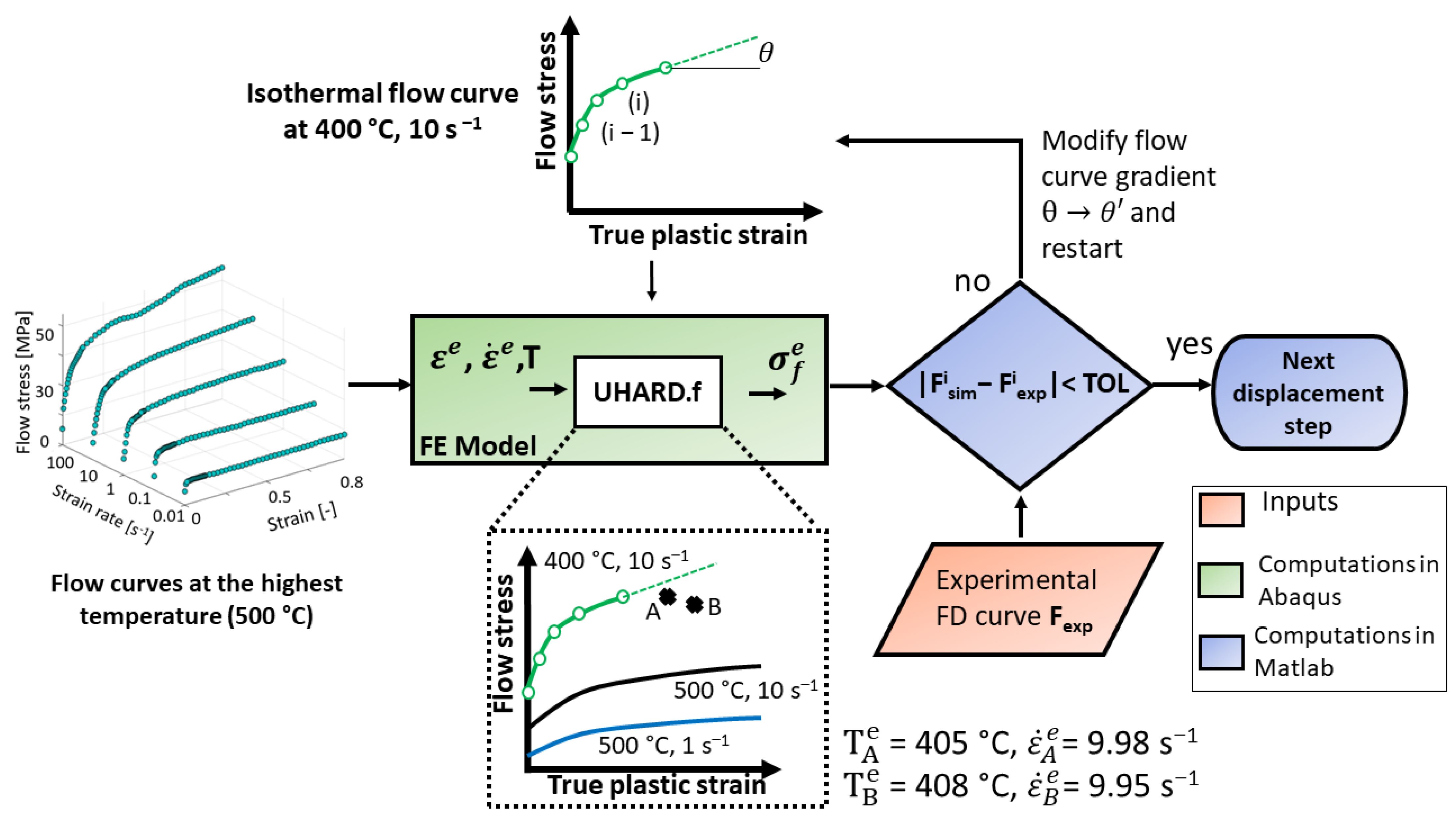
3. Methods and Procedure

This chapter first introduces the compression test FE model and the general procedure to sample the experimental data. Since the piecewise flow curve determination is at the core of FepiM and its further extension, the FepiM approach developed earlier is briefly reviewed after. Finally, the extension to the FepiM method comprising of a two-step simulation-based online temperature compensation method is introduced in detail. In the first step of the temperature compensation, flow curves at the highest temperature are determined, and considering these as a reference, flow curves at a lower temperature are determined.

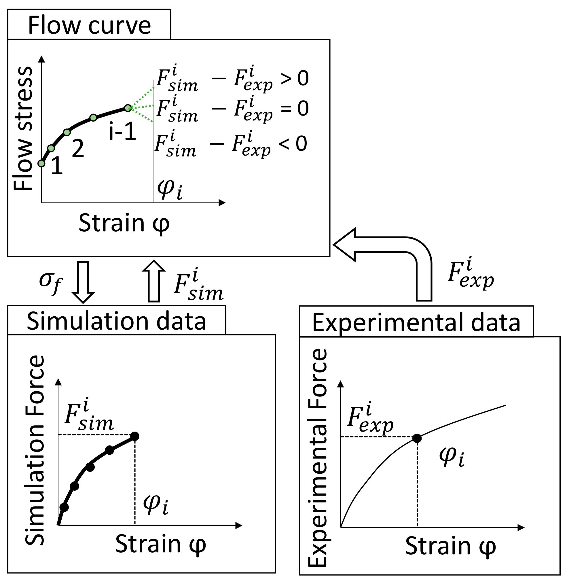
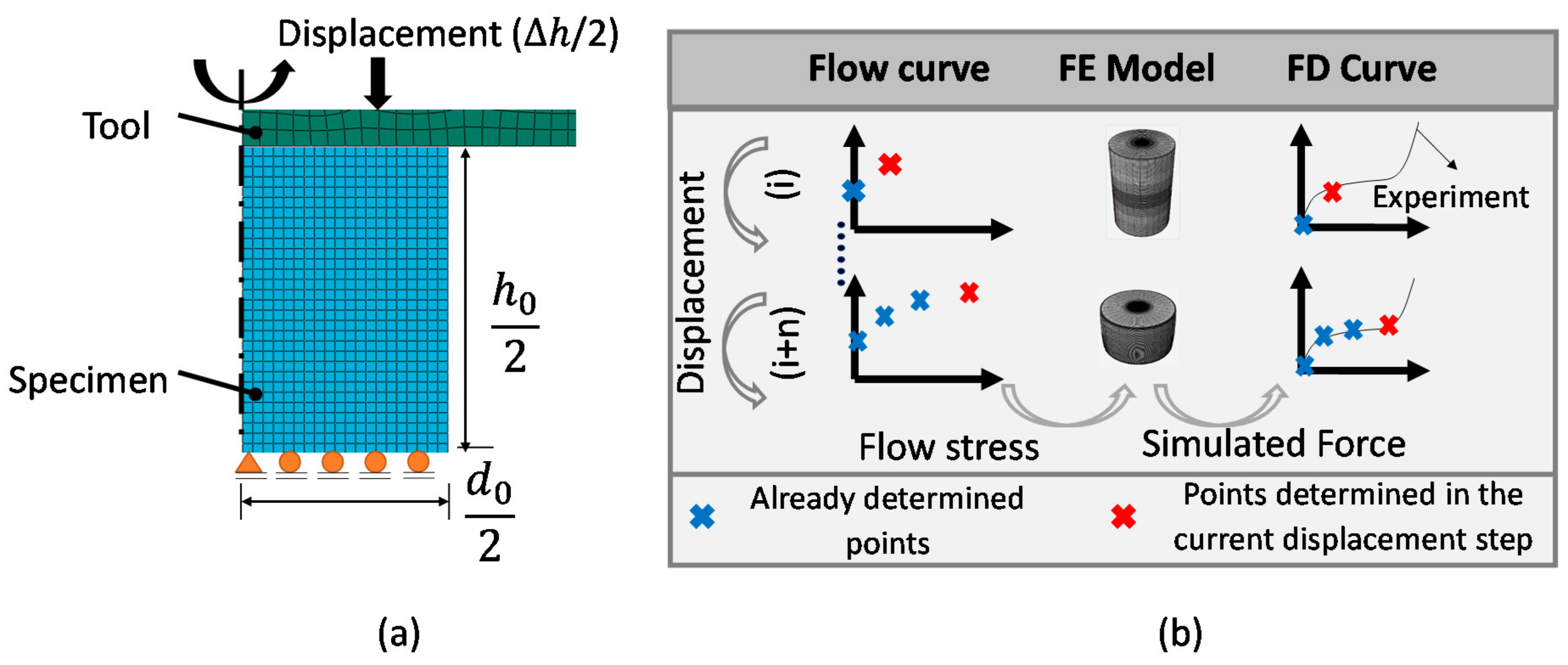
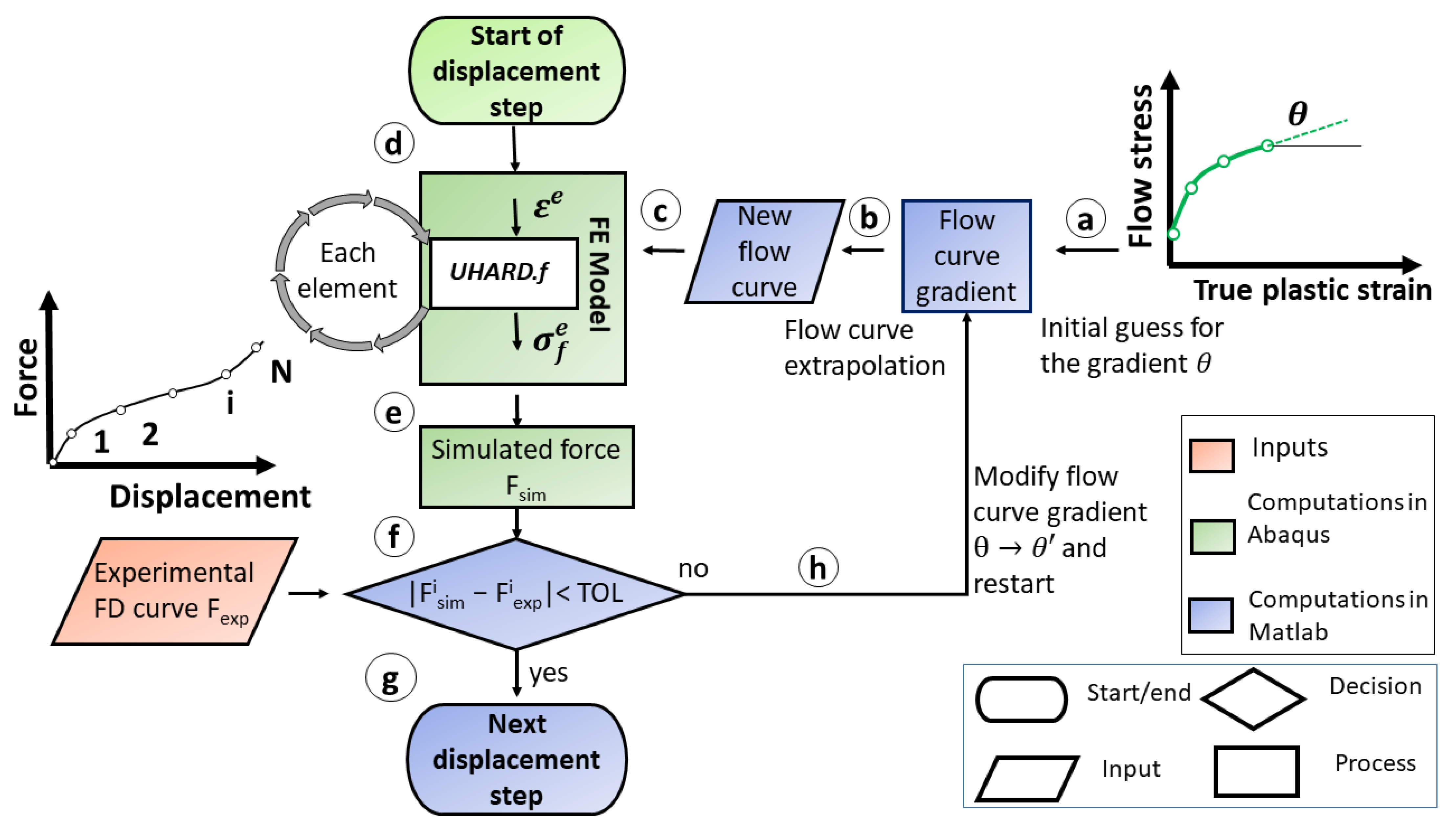
3.1. FE Model and Method of Consecutive Flow Curve Point Determination

The inverse flow curve determination is based on a FE model that mimics the experimental compression tests using the commercial FE software Abaqus/Standard 2016. Considering the geometrical symmetry, only one quarter of the actual compression test specimen is modeled. Moreover, its rotational symmetry is exploited, and thus a 2D axisymmetric model suffices. The FE model is shown in Figure 2a. Coulomb friction and interfacial heat transfer coefficient (IHC) are defined between the tool and specimen. At the beginning of the simulation, each element in the model is assigned the nominal testing temperature ${\mathrm{T}}_{\mathrm{testing}}$, and a temperature increase might occur during simulation due to deformation heating in the specimen. In the current paper, the workpiece is discretized with an element size of 0.3 mm. As Rastegaev samples and a lubricant are used, a low friction coefficient of 0.005 is used between tool and work piece while an IHC of 0.004 W/(K mm²) is used at the metal-ceramic interface which is adopted from [10]. A dissipation coefficient of 0.95 is used.

FepiM employs the abovementioned FE model to determine the piecewise flow curve. The yield stress and the experimental force displacement (FD) curve are given as an input to FepiM. The FD curve is then sampled into different displacement steps. An optimal flow curve point comprised of flow stress and plastic strain is determined at each displacement step such that the error between the experimental and simulated force is minimal. These flow curve points are sequentially determined up until the full displacement is captured and each flow curve point in the output flow curve corresponds to one displacement step in the sampled FD curve. This method is also illustrated in Figure 2b. It is important to note that sequential also implies that once determined flow curve points are fixed henceforward and only the section of the flow curve with strains greater than the last displacement step is considered. In addition, using the Abaqus restart function enables the computation to progress with displacement like in a conventional simulation without the need for any recalculation. The exact procedure to obtain these optimal flow curve points is detailed in the subsection below. Determining a flow curve point at every point on the experimental FD curve can be redundant and computationally expensive. Instead, based on the severity of change in the slope of the FD curve, only some significant displacement steps are resampled and used. These resampled points are called evaluation points (EPs). For details on the procedure to obtain these EPs, the reader is referred to [18].

3.2. The FepiM Approach

The explicit piecewise flow curve determination approach FepiM employs an iterative scheme to determine the flow curve points and minimize the error between the experimental and simulated forces. The scheme for obtaining flow curve points is discussed below and is additionally illustrated via a block diagram in Figure 3. The input experimental FD curve is divided into a total of N Eps, and a flow curve point (${\mathsf{\phi }}^{\mathrm{j}},{\mathsf{\sigma }}_{\mathrm{f}}{}^{\mathrm{j}}$) (j = 1 to N) corresponding to each EP is determined.

The FepiM approach is implemented using the software package MATLAB R2018b. Thus, MATLAB scripts are used to control and perform iterations in Abaqus/Standard as well as to obtain optimal flow curve points, as discussed in more detail below. The UHARD [8] subroutine available within the Abaqus/Standard framework is used to link FepiM to Abaqus/Standard via the modification of the flow curve data as well as via assigning the flow stress to different elements in the model. The different steps involved in the iterative scheme for FepiM flow curve determination are discussed below. Here, it is assumed that the flow curve up until (${\mathsf{\phi }}^{\mathrm{j}},{\mathsf{\sigma }}_{\mathrm{f}}{}^{\mathrm{j}}$) (j = 1 to i) is known and does not change in further iterations.

Step (a) Initial gradient: To obtain a new flow curve point at the EP i + 1, the known flow curve (${\mathsf{\phi }}^{\mathrm{j}},{\mathsf{\sigma }}_{\mathrm{f}}{}^{\mathrm{j}}$) (j = 1 to i) must be extrapolated based on an initial gradient $\mathsf{\theta }$. This gradient is obtained by calculating the slope of the two previous flow curve points (${\mathsf{\phi }}^{\mathrm{j}},{\mathsf{\sigma }}_{\mathrm{f}}{}^{\mathrm{j}}$) (j = i and i − 1).

Step (b) Flow curve extrapolation: The flow curve (${\mathsf{\phi }}^{\mathrm{j}},{\mathsf{\sigma }}_{\mathrm{f}}{}^{\mathrm{j}}$) (j = 1 to i) is then extrapolated based on this gradient (up to a strain larger than encountered in this displacement step), and the whole flow curve is stored as an ASCII file.

Step (c) FE simulation step: The FE compression test simulation in Abaqus is performed for the given EP using the flow curve obtained in (b) as an input.

Step (d) Flow stress assignment: During the simulation, the UHARD subroutine integrated with the simulation obtains the plastic strain ${\mathsf{\epsilon }}^{\mathrm{e}}$ of every element in the FE model through the Abaqus framework. In turn, UHARD reads the flow curve data stored in the ASCII file and calculates the elements flow stress ${\mathsf{\sigma }}_{\mathrm{f}}^{\mathrm{e}}$ by linear interpolation. The necessity of using UHARD and storing the flow curve data in an ASCII is discussed below.

Step (e) Extraction of global simulated force: Then, at the end of the FE simulation step the global simulated force (${\mathrm{F}}_{\mathrm{sim}}^{\mathrm{i}}$) is extracted.

Step (f) Force comparison and convergence check: ${\mathrm{F}}_{\mathrm{sim}}^{\mathrm{i}}$ is compared to the experimental force ${\mathrm{F}}_{\exp }^{\mathrm{i}}$ at the EP. If the absolute error between the simulated and the experimental force is converged to a user-defined tolerance limit (+/−2 N is used in this paper), the iterations are stopped; otherwise, further iterations are performed.

Step (g) Modifications for optimal gradient $\mathsf{\theta }$: If convergence is not achieved in (f), then (b) to (f) are repeated with a new gradient $\mathsf{\theta }\to {\mathsf{\theta }}^{\prime }$. The new gradient is calculated with respect to the relative error between the experimental and simulated force

$${\mathsf{\theta }}^{\prime }=\mathsf{\theta }+\mathrm{H} ({\mathrm{F}}_{\exp }^{\mathrm{i}}-{\mathrm{F}}_{\mathrm{sim}}^{\mathrm{i}}).$$

(5)

H is a user-defined parameter affecting convergence. If H is too small, the number of iterations for convergence is high, and if it is too large, the predicted gradient exceeds the optimal value and causes instabilities in the further simulation.

Step (h) Progress to next EP: After convergence in (f), the point on the extrapolated flow curve section corresponding to the current EP is obtained. This is done by identifying the element with the maximum plastic strain in the FE model and choosing its corresponding von Mises stress as a new flow curve point. FepiM then progresses to the next EP, and the sequence from (a) to (g) is repeated for each displacement step until j = N is reached.

The Abaqus restart functionality is used to move to the next EP after convergence in (f). This avoids rerunning the simulation from the first EP again. However, because Abaqus restricts changing material data during restarts, a separate UHARD is developed where the flow curve data stored as an ASCII file is read during simulations, and after each displacement step, the optimized new flow curve point is added to the flow curve file.

The iterative FepiM scheme was tested and showed good accuracy when determining flow curves with a strain inhomogeneity in the specimen during deformation [18]. Here, the FepiM approach is further exploited to determine flow curves when there is a temperature inhomogeneity in the specimen due to deformation heating alongside the strain inhomogeneity already considered. This requires further extension of the algorithm to handle these severely inhomogeneous conditions and to determine isothermal flow curves from experimental data.

3.3. Stepwise Flow Curve Determination Procedure

As discussed already, some level of temperature inhomogeneity in the specimen can be expected due to the heat transfer to the tool as well as to the environment. This also implies an inhomogeneity in strength and thus strain and also strain rate. Therefore, isothermal, constant strain rate flow curves cannot be determined using the method introduced in the previous section and shown in Figure 3. Commonly, the force-displacement curves from different experiments are converted to flow curve data and then the flow curve field is temperature compensated offline by linearly interpolating between the flow curve data obtained from other temperatures. Opposed to conventional flow curve determination, here, isothermal flow curves are determined through online temperature compensation where temperature inhomogeneity in the specimen is also considered. For that, a stepwise procedure is incorporated into FepiM where flow curves are determined starting from the highest temperature. This way, flow curves at the higher temperature act as a reference for the temperature compensation to determine the flow curves at lower temperatures.

In the first step of the procedure, i.e., for the flow curves at the highest temperature there is no reference available to compensate for the decrease in flow stress due to the temperature rise. Hence, these flow curves must be handled separately from the other flow curves. In the subsections below, the procedure for the highest temperature and strain rate flow curves is introduced first followed by the procedure for lower temperatures and strain rates. To keep things simple, the procedure is exemplified via a flow curve field consisting of only two temperatures (500 and 400 °C) and two strain rates of 10 s⁻¹ and 1 s⁻¹.

3.3.1. Determination of Flow Curves at the Highest Temperature and Strain Rate

The conventional piecewise flow curve determination illustrated in Figure 3 is combined with an analytical temperature compensation method to determine flow curves at the highest temperature, i.e., 500 °C. The experimental FD curve determined at ${\mathrm{T}}_{\mathrm{testing}}$ = 500 °C is used, and all the elements in the FE model are initially set to this temperature. At each EP, in addition to the flow curve point determination, the interpolated element temperature available as an output from the FE simulation is considered and averaged over the whole specimen. Now, to correct the flow stress due to the temperature change during deformation, a separate FE model at the closest lower temperature (here ${\mathrm{T}}_{\mathrm{testing}}$ = 400 °C) is built, and its corresponding flow curve and the average specimen temperature are determined independently as well. For illustration, two flow curves with a strain rate of 10 s⁻¹ starting at 500 °C (red) and 400 °C (blue) as well as their respective average temperature increase are shown in Figure 4. Then, the desired temperature compensated flow curve at 500 °C (green) is determined using Equation (4) in Section 1. This procedure is repeated for all strain rates to obtain all flow curves at the highest temperature.

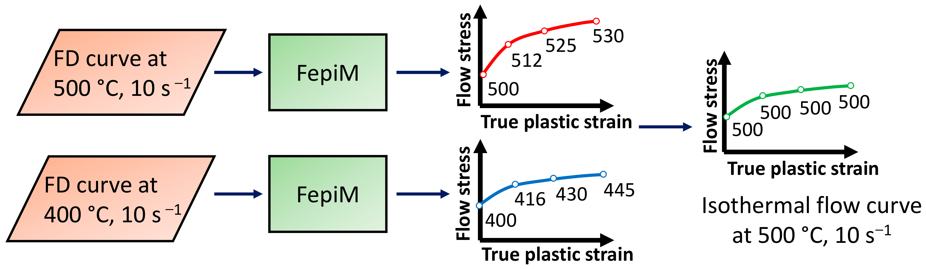
3.3.2. Determination of Flow Curves at Lower Temperatures and Strain Rates

For temperatures other than the highest, an online temperature compensation concept is used where the flow curve points corresponding to the nominal testing temperature are determined directly from the simulation. This is achieved by incorporating an extra interpolation layer for temperature into the FepiM approach discussed in Section 2.2. The procedure is illustrated in Figure 5 and discussed hereafter based on the determination of the flow curve at 400 °C, 1 s⁻¹. As discussed in Section 2.2, the flow curve considered (here 400 °C, 10 s⁻¹) is initially extrapolated to a sufficiently large strain using the gradient $\mathsf{\theta }$. This flow curve and all the flow curves at the highest temperature (here 500 °C) are imported into the UHARD subroutine. During deformation, due to deformation heating, the temperature of the individual elements in the specimen then rises above the nominal temperature of 400 °C. The UHARD subroutine thus assigns flow stress to these elements by linearly interpolating between the flow curves at 500 °C and the new 400 °C, 1 s⁻¹ flow curve. For example, the temperatures at elements A and B in Figure 5 are 405 and 408 °C, respectively. After flow stress assignment, the global simulated force is compared to the sampled experimental force, again in accordance with Section 2.2. The iterations are stopped if the error is below the user-defined tolerance limit; otherwise, the procedure is repeated with a modified gradient $\mathsf{\theta }\to {\mathsf{\theta }}^{\prime }$ until convergence. After convergence, the maximum plastic strain at the EP is used to store the final flow curve point on the curve at 400 °C, 10 s⁻¹, and the flow curve is added to the known flow curve field.

Similarly, also the strain rate is interpolated for all elements that differ from the nominal rate (10 s⁻¹ in this example). This is also shown in Figure 5 for points A and B with strain rates of 9.98 s⁻¹ and 9.95 s⁻¹, respectively. N.b., no extrapolation is performed for temperatures or strain rates outside of the know flow curves. Temperatures below 400°C and strain rates above 10 s⁻¹ would be mapped to the 400 °C, 10 s⁻¹ flow curve instead.

The procedure detailed above is repeated for the remaining temperatures and strain rates to obtain a complete flow curve field. In summary, it determines isothermal flow curves at constant strain rate, where the data points on the curves correspond to a desired nominal temperature and strain rate.

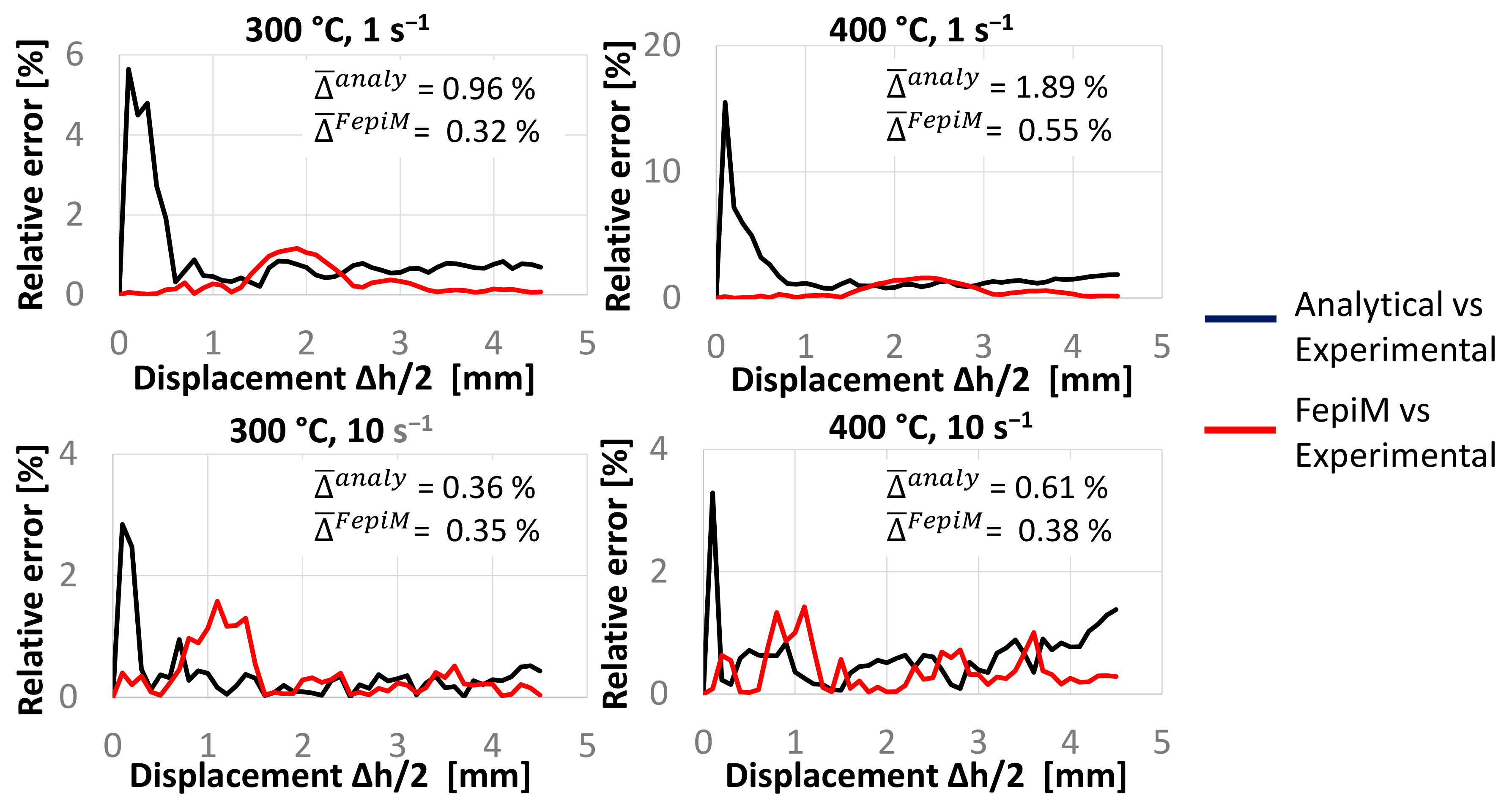
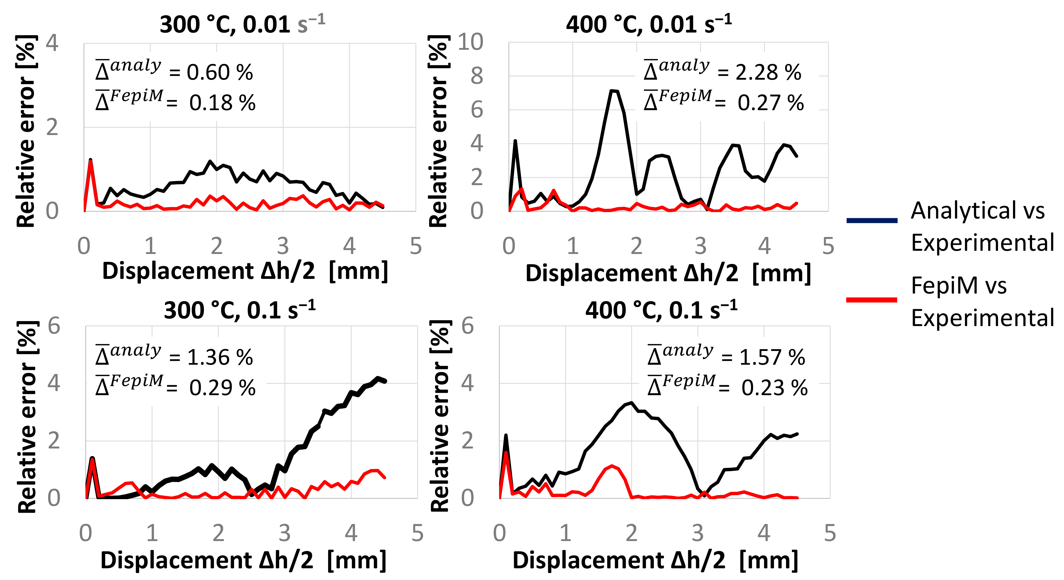
4. Results/Practical Examples

In this section, the application of FepiM is demonstrated by determining flow curves for two different metal alloys. Pure aluminum (AA1050) and electrolytically refined copper (Cu ETP) were chosen, considering their distinctly different flow curve shapes. The experiments to determine the corresponding FD curves are described first. Furthermore, this section seeks to validate the accuracy and robustness of the FepiM algorithm. To achieve this, FepiM is compared against the conventional analytical approach by Kopp et al. [10]. This approach was chosen as it provides good accuracy in most cases, especially for the conducted compression test employing Rastegaev samples. The results for both materials are presented in two separate subsections.

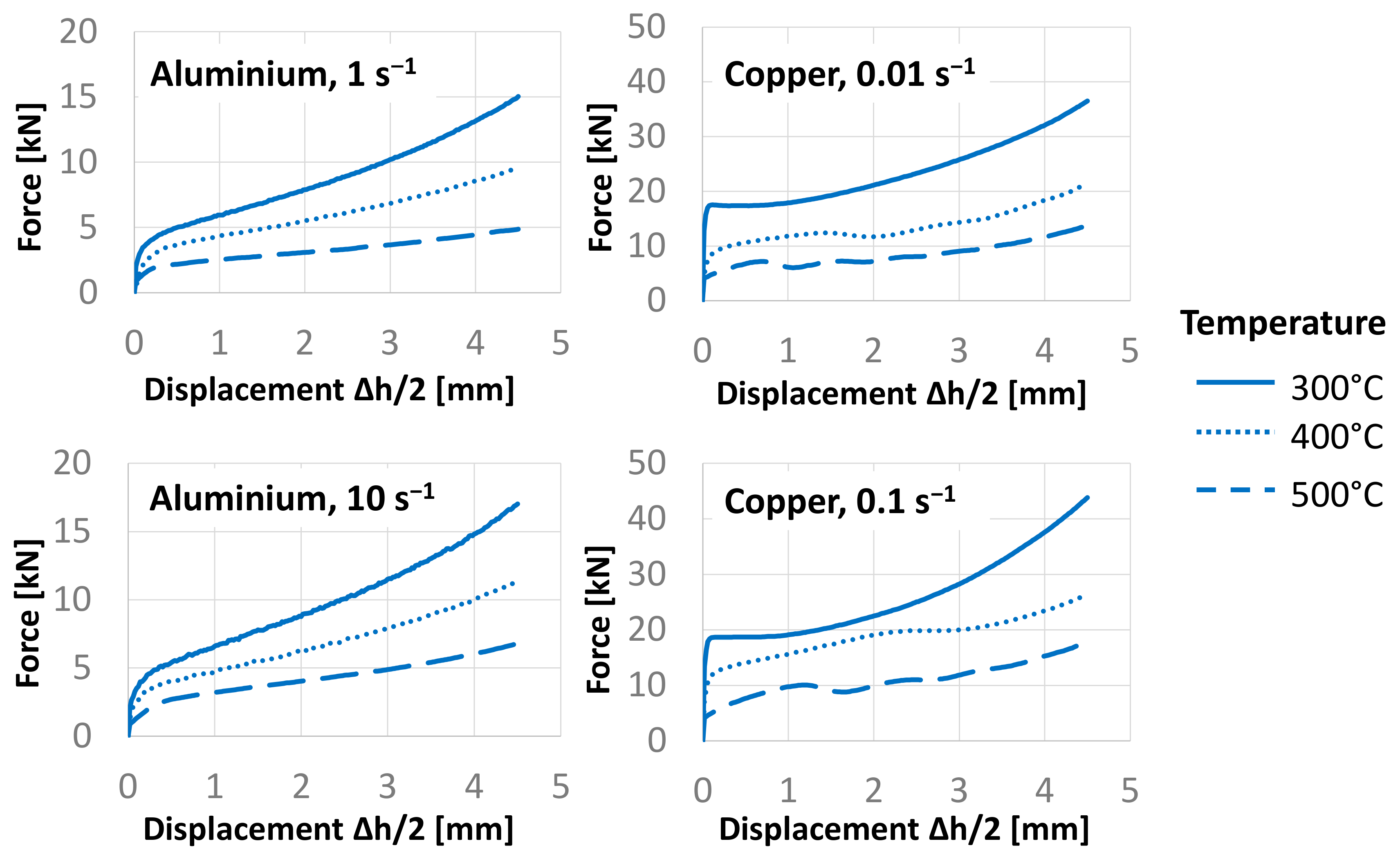
4.1. Compression Tests

The FD curves used to determine flow curves via FepiM, were recorded for the strain rates of 0.01 s⁻¹, 0.1 s⁻¹,1 s⁻¹, 10 s⁻¹, 100 s⁻¹ for aluminum and 0.01 s⁻¹, 0.1 s⁻¹, and 1 s⁻¹ for copper and at the nominal testing temperature of 20, 100, 200, 300, 400, and 500 °C through cylindrical compression tests using specimen of 12 × 18 mm and 10 × 15 mm diameter and height for aluminum and copper, respectively. A Servo-hydraulic testing machine (“Servotest”) is used to perform the trials. The compression tool along with the specimen is enclosed in an isothermal furnace, ensuring that the test setup is at a nominal testing temperature as the experiment starts and that the specimen temperature never drops below the nominal testing temperature during the test. Friction is minimized by using Rastegaev specimens and a Teflon lubricant. The experimental FD curves for aluminum at 500, 400, and 300 °C and strain rates of 1 s⁻¹ and 10 s⁻¹ as well as for copper at 500, 400, and 300 °C and strain rates of 0.01 s⁻¹ and 0.1 s⁻¹ are shown in Figure 6. In accordance with the FE model, the displacement in the FD curves is displayed as one half the of the tool displacement. The FD curves of aluminum show a monotonous increase, whereas for copper a more complex non-monotonous behavior is visible.

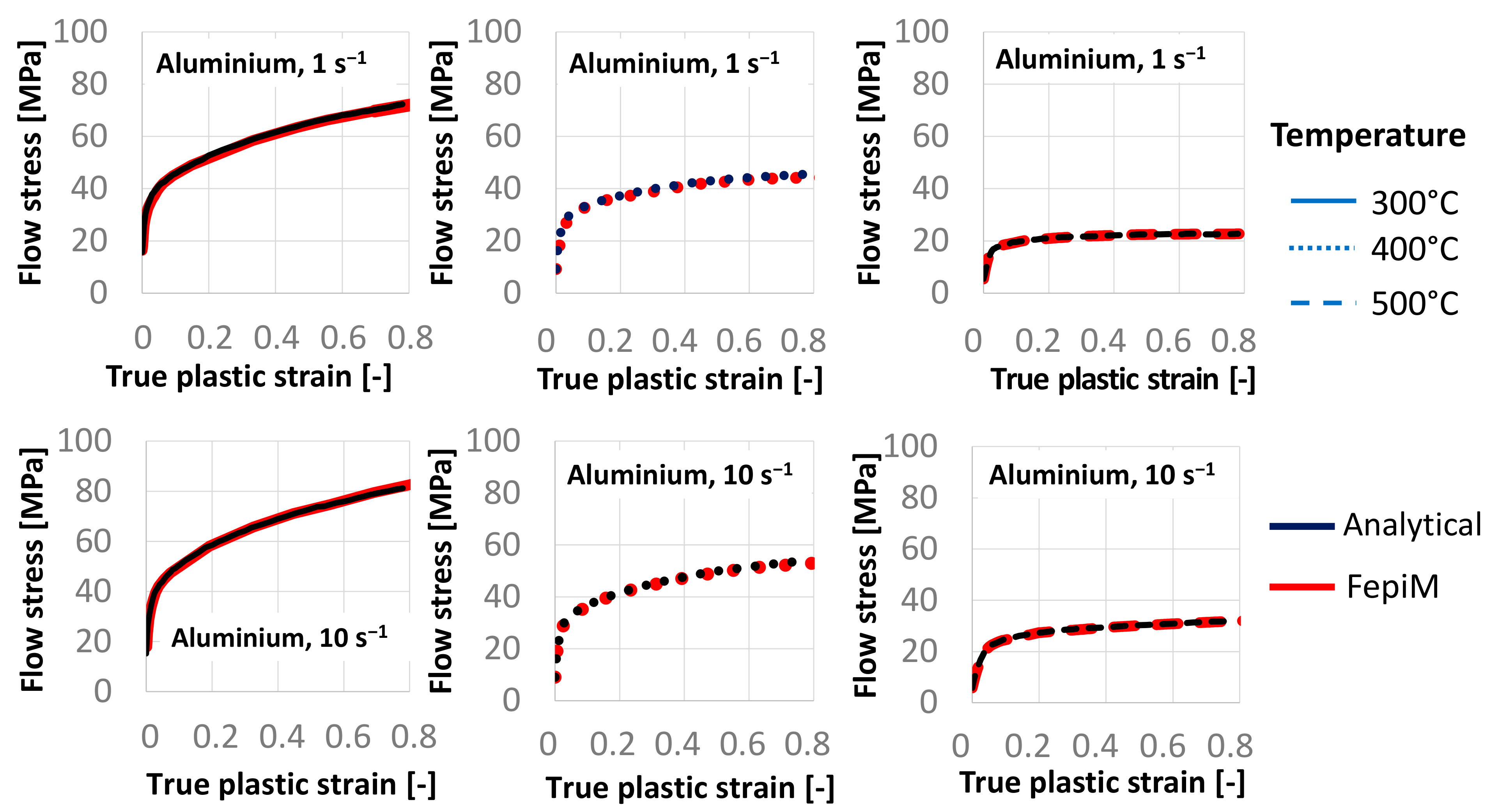
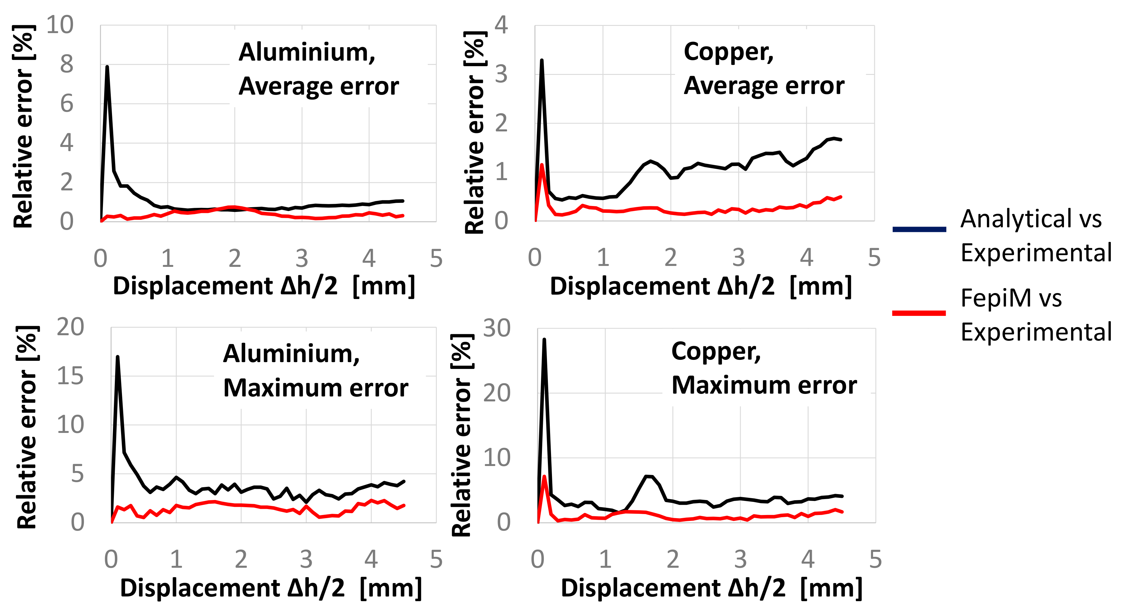
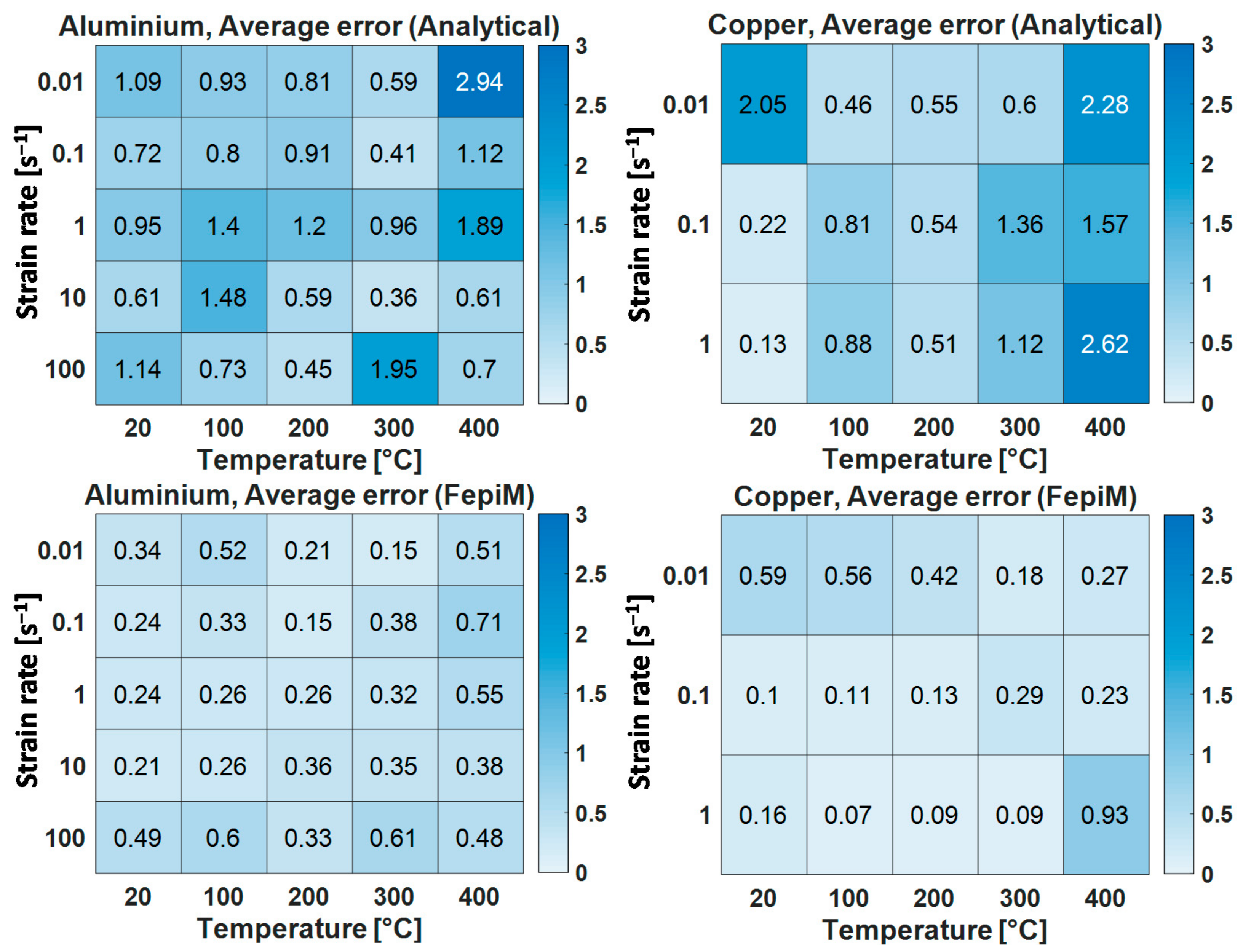
4.2. FepiM Flow Curves for Aluminum

The flow curves for aluminum were determined according to the procedure introduced above starting with the flow curve at 500 °C and 100 s⁻¹ and ending with the flow curve at 20 °C and 0.01 s⁻¹. Some resulting FepiM and temperature-compensated analytical flow curves for three temperatures (500, 400, and 300 °C) and two strain rates (1 s⁻¹ and 10 s⁻¹) are shown in Figure 7. It can be seen in the figure that aluminum flow curves show monotonic hardening and that the FepiM flow curves mostly match the analytical flow curve. A thorough comparison of analytical and FepiM flow curves with respect to the experimental are presented below in Section 4.

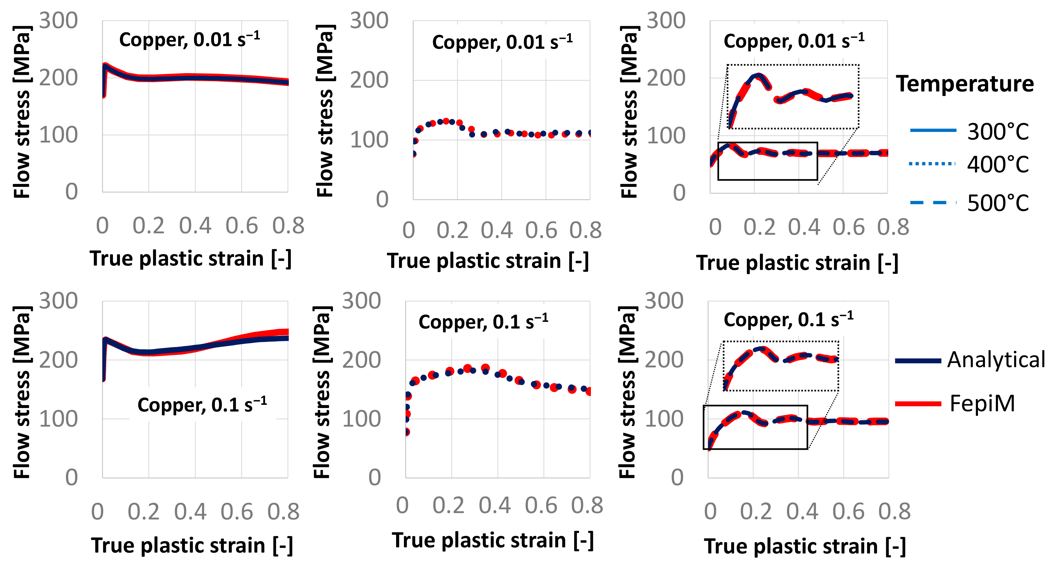
4.3. FepiM Flow Curves for Copper

Using the FepiM approach, additional flow curves for copper between 20 °C to 500 °C and strain rates of 0.01 s⁻¹, 0.1 s⁻¹, and 1 s⁻¹ were determined. In Figure 8, the flow curves determined with FepiM are shown in comparison to the analytically determined flow curves for temperatures of 500, 400, and 300 °C and 0.01 s⁻¹, 0.1 s⁻¹ strain rates. The nonmonotonous hardening of copper especially at higher temperatures where dynamic recrystallization with multiple peaks occurs is well captured by the flow curves determined with FepiM. While the analytical approach also captures the complex hardening, it would be difficult to mimic such behavior based on conventional inverse modeling approaches where a matching empirical flow curve equation is required. Again, an in-depth analysis of the flow curves is given below in Section 4.

5. Discussion

This section presents a quantitative analysis of the FepiM and the analytical flow curves. However, before presenting the details, it is important to state that for compression tests a very good agreement of FepiM and analytical flow curves is to be expected. This is already obvious from the results presented above and as previously mentioned is caused by the comparably low inhomogeneity in the compression specimen. However, the detailed analysis presented hereafter is only feasible because a precise analytical assessment of the hot compression tests is possible. The same comparison and thus validation would be impossible for inhomogeneous torsion tests, as analytical analysis methods fail to obtain precise results for these tests.

For the quantitative analysis simulations of the compression tests replicating, all experiments conducted in Section 3 are performed using the same FE model as for the inverse flow curve determination. The entire flow curve fields identified before are fed into the simulations. This analysis allows for a direct comparison of the simulated FD curves with the experimental data and the analysis of the accuracy of FepiM method and the analytical method with temperature compensation. The relative error ($\left|\mathsf{\Delta }\right|=({\mathrm{F}}_{\mathrm{simulation}}-{\mathrm{F}}_{\mathrm{experimental}})/{\mathrm{F}}_{\mathrm{experimental}}·100$) between the simulated and experimental FD curves is used as a measure of accuracy.

In Figure 9 and Figure 10, the relative error between the simulated (via analytical and FepiM flow curves) and experimental FD curves for aluminum and copper is shown, respectively. To illustrate the evaluation, only the error for the experiments conducted at a nominal temperature of 300 and 400 °C is shown. When simulating the experiments conducted at a nominal temperature of 500 °C, the specimen temperature increases above 500 °C during compression, but since the isothermal flow curves above 500 °C are not available, a similar evaluation is not possible for these experiments.

As shown in Figure 9 for aluminum, the relative error in the FepiM flow curves is sometimes higher than the error in the analytical flow curves, e.g., for the 300 °C, 10 s⁻¹ case between displacement of 0.5 and 1.5 mm the error in the FepiM flow curves (red) is above the error in analytical flow curve (black). However, this error never exceeds 2% and therefore is acceptable. At the same time, this error can be further reduced by choosing more EPs during the flow curve evaluation but at the cost of computational time. Nevertheless, the overall average relative error ($\overline{\mathsf{\Delta }}$) over the whole displacement is smaller for FepiM in all four cases shown, i.e., between 0.32–0.55% for FepiM compared to 0.36–1.89% for the analytical flow curves. The relative error in the analytical flow curves reaches a maximum value at the beginning; notably, for the 400 °C, 1 s⁻¹ case, a maximum error of 16% is observed, and this error drops to below 2% as the simulation progresses. Simultaneously, the error in the FepiM flow curves is near constant. This is because the online temperature compensation method in FepiM allows flow curve evaluation considering the inhomogeneity in temperature, whereas the analytical flow curves are determined by averaging the temperature over the specimen.

In the case of copper shown in Figure 10, the average relative error in the FepiM flow curves is again low, ranging around 0.18–0.29%, whereas the error in the analytical flow curves is between 0.6–2.3%. A maximum error of around 7% is observed in the analytical flow curve at 400 °C, 0.01 s⁻¹, and the error fluctuates as the simulation progresses, while the error in the FepiM flow curves is below 2% throughout. As for aluminum, in most cases, the error in the analytical flow curves increases with displacement, whereas the error in the FepiM flow curves is rather constant and lies below the analytical flow curves almost everywhere.

Additionally, the same analysis was performed for all experimental conditions (0.01 s⁻¹, 0.1 s⁻¹,1 s⁻¹, 10 s⁻¹, and 100 s⁻¹ for aluminum and 0.01 s⁻¹, 0.1 s⁻¹, and 1 s⁻¹ for copper and at the nominal testing temperatures of 20, 100, 200, 300, 400, and 500 °C). The relative error in dependence of displacement is calculated in each case with respect to the analytical and FepiM flow curves. From this analysis, the average error and the maximum error over the displacement is obtained and plotted in Figure 11. The average and maximum error for the FepiM flow curves is consistently low compared to the analytical flow curves. This analysis can provide intuition on the accuracy of the flow curves when using the complete flow curve field in a process simulation. The maximum error of 17% at the beginning in the analytical flow curve for the aluminum case is caused by the 100 °C, 10 s⁻¹ flow curve, while the 30% at the same point in the copper case corresponds to the 400 °C, 1 s⁻¹ flow curve; both of which are not displayed in Figure 9 and Figure 10.

In Figure 12, the average relative error ($\overline{\mathsf{\Delta }}$) is shown for each experimental condition in a heatmap. The error is calculated with respect to the experimental FD curve for both aluminum and copper. It is observed that the average error for the FepiM flow curves is always below 1% for all the conditions, whereas the error in the analytical flow curves is higher with a maximum average error of around 3%.

Overall, the robustness of FepiM was assessed based on flow curves determined for two different materials with distinctly different flow curve shapes. The FepiM curves were compared to analytically determined flow curves. As seen, the FepiM flow curves were on par with or slightly better than the analytical curves for most cases. The slight advantage of FepiM is expected, as it explicitly considers the temperature inhomogeneity in the specimen and that is captured only in an average sense in the analytical methods [10]. Additionally, flow curves with several recrystallization cycles are reproduced well, which is difficult to achieve using conventional inverse modeling based on flow curve equations [5]. Finally, the FepiM approach proved to be more versatile than other piecewise approaches like IFD [16], as it was successfully applied to compression tests where a strain measurement inside the specimen using DIC is impossible.

6. Conclusions and Future Scope

This paper extends the applicability of the FepiM approach developed earlier to flow curves obtained at elevated temperatures. Generally, the FepiM approach can do without explicit and sophisticated strain measurements like DIC while at the same time overcoming the limitations of conventional inverse modeling where an empirical flow curve equation is required a priori. The FepiM approach is extended by a two-step strategy to determine an entire isothermal flow curve field for hot working applications. In the first step, the flow curves at the highest temperature are determined using a combined piecewise and analytical approach, and in the second step, these flow curves are used as references to determine the flow curves at all lower temperatures. The temperature compensation method can consider temperature and strain rate inhomogeneity online while determining the flow curves without further postprocessing. Flow curves for aluminum and copper were determined, and the force-displacement curves derived from simulations using FepiM flow curves showed an error between 0.1–1%, whereas the flow curves determined by the analytical method showed an error between 0.1–3%.

Here, only compression tests based on Rastegaev samples were considered. These trials prevent friction and do not entail distinct temperature inhomogeneity. Thus, no great differences between the FepiM results and the analytical analysis were to be expected. However, the FepiM results were always on par with the analytical ones and often even superior. The advantages are expected to further increase for experimental conditions with much larger inhomogeneity. Thus, the longer-term aim is to apply the FepiM approach to determine flow curves from compression tests without lubrication and then adopt the approach to other material testing methods like tensile tests with high strain inhomogeneity due to necking [5] for torsion tests with equally high strain and strain rate inhomogeneity along the radial direction [4] during deformation and where analytical simplifications do not hold.

References

1. Dieter, G.E. Bulk Workability Testing: Chapter 4. In Handbook of Workability and Process Design; Dieter, G.E., Kuhn, H.A., Semiatin, S.L., Eds.; ASM: Novelty, OH, USA, 2003; pp. 47–56. ISBN 0-87170-778-0. [Google Scholar]
2. Goetz, R.L.; Semiatin, S.L. The Adiabatic Correction Factor for Deformation Heating during the Uniaxial Compression Test. J. Mater. Eng. Perform. 2001, 10, 710–717. [Google Scholar] [CrossRef]
3. Poehlandt, K. Materials Testing for the Metal Forming Industry; Springer: Berlin/Heidelberg, Germany, 1989; ISBN 0-387-50651-9. [Google Scholar]
4. Khoddam, S.; Hodgson, P.D. Conversion of the hot torsion test results into flow curve with multiple regimes of hardening. J. Mater. Process. Technol. 2004, 153–154, 839–845. [Google Scholar] [CrossRef]
5. Tu, S.; Ren, X.; He, J.; Zhang, Z. Stress–strain curves of metallic materials and post-necking strain hardening characterization: A review. Fatigue Fract. Eng. Mater. Struct. 2020, 43, 3–19. [Google Scholar] [CrossRef] [Green Version]
6. Rastegaev, M.V. Neue Methoden der homogenen Stauchung von Proben zur Bestimmung der Fließspannung und des Koeffizienten der inneren Reibung. Zavod. Lab. 1940, 3, 354–355. [Google Scholar]
7. Zhao, D. Testing for Deformation Modeling. In Mechanical Testing and Evaluation: ASM Handbook; Kuhn, H.A., Medlin, D., Eds.; ASM International: Russell Township, OH, USA, 2000; pp. 798–810. ISBN 978-0-87170-389-7. [Google Scholar]
8. Smith, M. ABAQUS/Standard User’s Manual, Version 6.9; Dassault Systemes Simulia Corp: Providence, RI, USA, 2009. [Google Scholar]
9. Lohmar, J.; Bambach, M. Influence of Different Interpolation Techniques on the Determination of the Critical Conditions for the Onset of Dynamic Recrystallisation. Mater. Sci. Forum 2013, 762, 331–336. [Google Scholar] [CrossRef]
10. Kopp, R.; Luce, R.; Leisten, B.; Wolske, M.; Tschirnich, M.; Rehrmann, T.; Volles, R. Flow stress measuring by use of cylindrical compression test and special application to metal forming processes. Steel Res. 2001, 72, 394–401. [Google Scholar] [CrossRef]
11. Laasraoui, A.; Jonas, J.J. Prediction of steel flow stresses at high temperatures and strain rates. Metallurg. Mater. Trans. A 1991, 22, 1545–1558. [Google Scholar] [CrossRef]
12. Xiong, W.; Lohmar, J.; Bambach, M.; Hirt, G. A new method to determine isothermal flow curves for integrated process and microstructural simulation in metal forming. Int. J. Mater. Form. 2015, 8, 59–66. [Google Scholar] [CrossRef]
13. Solhjoo, S.; Khoddam, S. Evaluation of barreling and friction in uniaxial compression test: A kinematic analysis. Int. J. Mech. Sci. 2019, 156, 486–493. [Google Scholar] [CrossRef]
14. Forestier, R.; Massoni, E.; Chastel, Y. Estimation of constitutive parameters using an inverse method coupled to a 3D finite element software. J. Mater. Eng. Perform. 2002, 125–126, 594–601. [Google Scholar] [CrossRef]
15. Cao, J.; Li, F.; Ma, W.; Li, D.; Wang, K.; Ren, J.; Nie, H.; Dang, W. Constitutive equation for describing true stress–strain curves over a large range of strains. Philos. Mag. Lett. 2020, 100, 476–485. [Google Scholar] [CrossRef]
16. Kamaya, M.; Kawakubo, M. A procedure for determining the true stress–strain curve over a large range of strains using digital image correlation and finite element analysis. Mech. Mater. 2011, 43, 243–253. [Google Scholar] [CrossRef]
17. Zhao, K.; Wang, L.; Chang, Y.; Yan, J. Identification of post-necking stress–strain curve for sheet metals by inverse method. Mech. Mater. 2016, 92, 107–118. [Google Scholar] [CrossRef]
18. Vuppala, A.; Krämer, A.; Braun, A.; Lohmar, J.; Hirt, G. A New Inverse Explicit Flow Curve Determination Method for Compression Tests. Procedia Manuf. 2020, 47, 824–830. [Google Scholar] [CrossRef]
Figure 1. Illustration of piecewise flow curve determination based on the concept put forward by Kamaya et al. [16].
Metals 11 00602 g001
Figure 2. (a) Schematic of the finite element (FE) Model and (b) illustration of the concept of consecutive flow curve point determination.
Metals 11 00602 g002
Figure 3. Block diagram of the iterative scheme in flow curve determination through explicit piecewise inverse modeling (FepiM).
Metals 11 00602 g003
Figure 4. Block diagram for the flow curve determination at the highest temperature and strain rate.
Metals 11 00602 g004
Figure 5. Block diagram for flow curve determination at lower temperatures and strain rates.
Metals 11 00602 g005
Figure 6. Example force displacement (FD) curves for aluminum and copper at three temperatures and two strain rates.
Metals 11 00602 g006
Figure 7. Flow curves for aluminum at different temperatures and strain rates.
Metals 11 00602 g007
Figure 8. Flow curves for copper at different temperatures and strain rates.
Metals 11 00602 g008
Figure 9. Validation analysis for some aluminum flow curves.
Metals 11 00602 g009
Figure 10. Validation analysis for some copper flow curves.
Metals 11 00602 g010
Figure 11. The average and maximum relative error for the complete flow curve field for aluminum and copper.
Metals 11 00602 g011
Figure 12. Relative average error for the complete flow curve fields.
Metals 11 00602 g012
Publisher’s Note: MDPI stays neutral with regard to jurisdictional claims in published maps and institutional affiliations.