Fatigue Models Based on Real Load Spectra and Corrected S-N Curve for Estimating the Residual Service Life of the Remanufactured Excavator Beam

Abstract

To more accurately predict the residual fatigue cycles and estimate the service life of the remanufactured excavator, the fatigue models integrating the corrected S-N curve, the RFC algorithm, the FEA model, and the mechanism dynamic model are established depending on the real load spectra under experimental working conditions and the corrected S-N curve of the beam metal remanufactured with the welding process. Depending on the test data of the unidirectional stress history and the servo displacements of the major cylinders, the mechanism dynamic model was first established to illustrate the real load spectra applied on the pivots of the working beam. The load spectra are further used in the finite element analysis (FEA) model to obtain the stress contours of the beam relevant to the sampling time, which is the stress spectra at any nodes on the beam in theory. Subsequently, the rain flow counting (RFC) algorithm based on the dual parameters of the cyclic stress amplitude and mean is established to provide the frequency spectra in the longevity region on the beam. Furthermore, due to the fatigue property changes of the beam metal remanufactured with the welding process, its S-N curve is corrected based on the detail fatigue rating (DFR) method to compute the stress cycles at each stress level on the crisis nodes. Finally, the total stress cycles that can be burdened by the remanufactured beam is computed under the Miner’s linear fatigue cumulative criterion. The total number of stress cycles is eventually converted to the fatigue and service life depending on the proportion of the sampling time under relevant working conditions. The results show that integrated fatigue models provide a practical approach to enhancing the accuracy of the estimation on the residual service life of the remanufactured excavator beam. It is significant for improving the reliability and safety of the remanufactured excavator.

1. Introduction

The core motivation of this paper is to use a comprehensive fatigue model based on the real load spectrum and the modified S-N curve to predict the residual life of the remanufactured excavator beam. China has prospered the market for remanufacturing engineering technology of construction machinery by promoting sustainable development strategy [1,2,3]. In this market, hydraulic excavators account for nearly one-third to half of the sales volume [4]. Therefore, improving the reliability of the remanufacturing excavator and prolonging its service life are of great significance to the quality improvement and market prosperity of the remanufacturing construction machinery. Excavator is now widely used in energy, mining, transportation, water conservancy, modern military engineering and other construction projects. The working conditions are very complex and these applications are often associated with torsional force bearing because the material is subject to variable loading conditions. The structural parts of the working device will suffer fatigue damage for a long time under the action of complex alternating loads. When the damage accumulates to a certain extent. This can lead to fatigue damage. A large number of studies have shown that more than 80% of component failures are caused by fatigue.

Structural fatigue is the main factor affecting the service life of machinery. The boom is one of the main components of the hydraulic excavator’s working device. It is a box structure welded with steel plates. The welding part is the part of the structure whose geometrical shape changes greatly. It is easy to produce stress concentration and fatigue crack. Therefore, it is often the place to evaluate the focus of life learning. Zhuang [5] evaluated the life of the front support part of the boom and optimized the support end of the cylinder. Cheng [6] adopts the nominal stress method to analyze the fatigue life of the hydraulic excavator working device based on the measured load. According to the actual product of the excavator. Jun [7] carried out dynamic modeling and simulation on the whole excavator working device. According to the simulation results, the dynamic stress fatigue reliability test of the actual excavator working device is carried out.

Actually, besides the dynamic properties effect on the accuracy of the estimation on fatigue life, many factors also affect it, such as the types and conditions of materials, geometric structures of components, variations of loads, and the complex states of stress while the machinery is under various working conditions [8]. Especially for the remanufactured components, the material mechanical property changes caused by the repair processes also take significant effects on the fatigue life estimation. Welding is the most usual repair process in remanufacturing. Suhir E. [9] studied the effect of elastic deformations on welding materials using the probabilistic principle-Miner rule. S.R. Sin used a quasi-static tensile-shear test to perform the fatigue analysis on a multi-lap spot welded joint of high strength steel and put forward a kind of method for measuring the fatigue life of high-strength steel plates with multi-lap spot welding [10]. All results showed that the mechanical properties of welding materials dramatically changed the fatigue life of the machinery.

As known, the S-N curve reflects the fatigue property of the material. Zhu [11] checked the static strength of the boom by simulating the load spectrum of each hinge point of the working device, predicted the fatigue life of the boom by miner criterion, and determined the minimum fatigue life position. Therefore, the S-N curve should be corrected for indicating the stress cycles of fatigue limit that can be burdened by the welding materials. Cheng introduced the classic method on the fatigue prediction for the working beam of the excavator, in which the factors of fatigue notch and coefficients of dispersion are seriously considered for correcting the S-N curve [6]. Many researchers developed various methods to improve the accuracy of the S-N curve considering various machinery structures and working conditions. Wang modified the S-N curves of metals by using the interval analysis model under the theory of non-probability set. It is easier to acquire a more accurate amplitude of equivalent stress even if the statistical data from the fatigue tests is insufficient [12]. Gao also established an empirical model upon the decreasing fatigue strength to simplify the test of the S-N curve with much fewer data samples than before, whatever for materials or components with given structures [13].

Either the S-N correction or the mechanism dynamic analysis both depends on the stress of the machinery and its changes. However, the stress depends on the real working load and responds to the machinery changes. That means the intensity, periodicity, frequency, and deviation of the working load under real working conditions and the corresponding stress fluctuation will remarkably affect the estimation of the fatigue life. Since they are critical to estimating the fatigue life for the machinery with a given material and structure, the time plots responding to the intensity of real working load and stress at critical points need to be established as the technical basis for the fatigue life prediction. Those plots relevant to the working loads at pivot points on components are called the load spectra and the corresponding stress plots at crisis points on components are called the stress spectra. In this paper, a dynamic model considering the real excavating conditions is proposed to simulate the real excavating loads and stress spectra. Subsequently, a fatigue property model for the remanufactured beam with welding structures is established by correcting the S-N curve. Consequently, the integrated fatigue models based on real load spectra and corrected S-N curves are employed for estimating the residual service life of the remanufactured excavator beam. These models facilitate the elevation of the estimation accuracy since more real conditions of loads and mechanism are considered besides the fatigue properties of the materials. Particularly the dynamic machinery model based on the real load spectra plays a remarkable role in accurately estimating the residual fatigue life of the excavator beam.

2. Materials and Methods

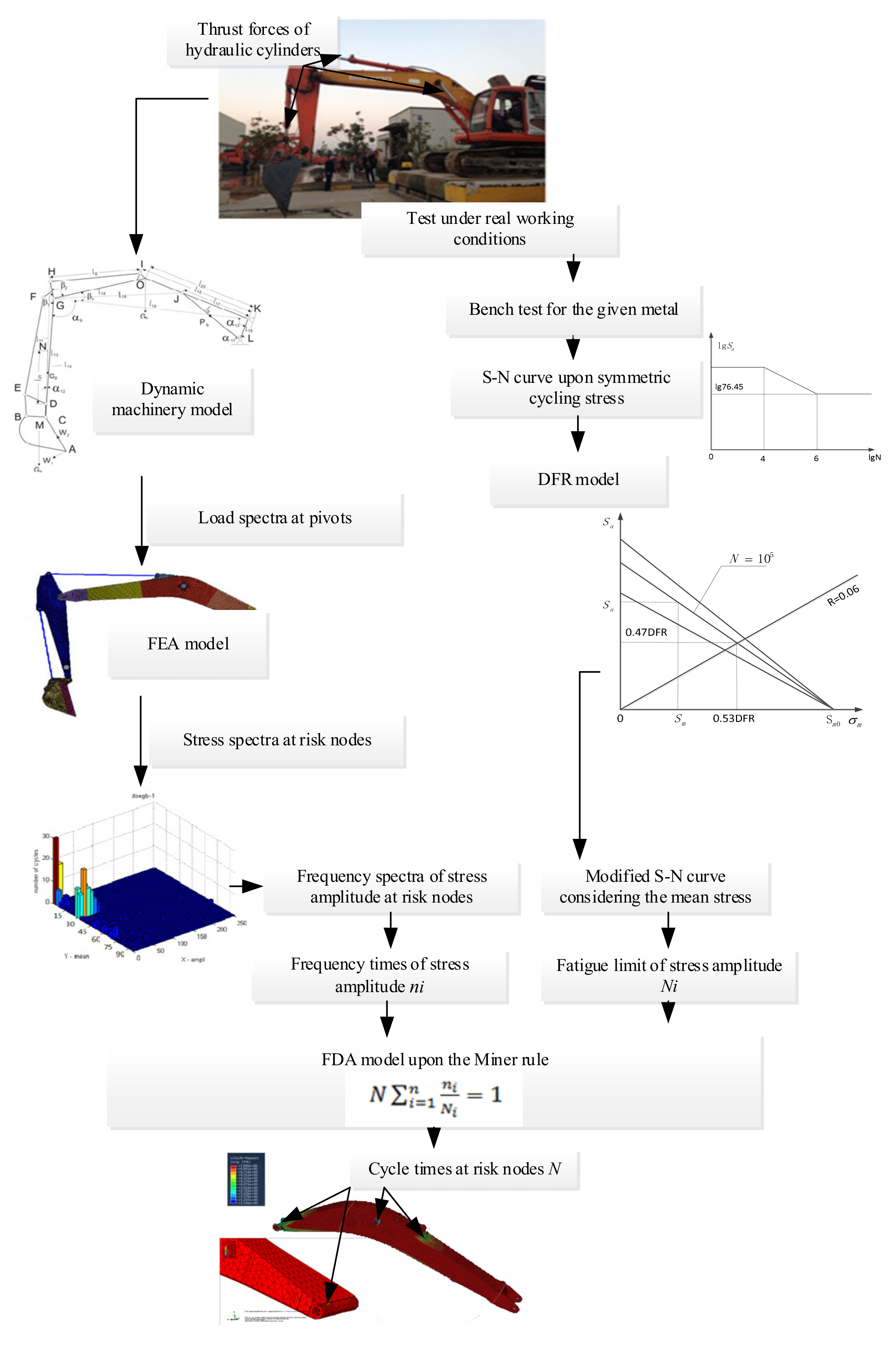
The Technical Framework and the Critical Models for the Fatigue Life Prediction

A series of fatigue models including the dynamic machinery model, the FEA model, the RFC algorithm, and the structural DFR model is established for predicting the fatigue life at risk points on the remanufactured beam of the hydraulic excavator. The dynamic machinery model simulates the load spectra at pivots of the excavator beam. Depending on the FEA model and reasonable boundary conditions, the load spectra are converted into the stress spectra at the risk points on the excavator beam. With the rain-flow counting (RFC) method, the frequency spectrum of the stress amplitude and mean is obtained depending on the stress spectrum. With the detail fatigue rating (DFR) model, the S-N curve based on the fatigue properties of metals is corrected via converting the non-zero mean stress to the equivalent symmetrical stress. The number of cycles of fatigue limit is decided depending on the stress amplitudes. Finally, the fatigue life is estimated based on the model of fatigue damage accumulation (FDA) upon the Miner rule. All critical models and methods are integrated to predict accurately the fatigue life of the excavator beam with considering the performances of remanufactured machinery and real working conditions. The technical framework of the fatigue life prediction on the excavator beam is illustrated in Figure 1.

Here are 2 critical models which one is the dynamic machinery model and the other one is the DFR model. Therefore, they form 2 technical routines to obtain the frequency times of stress amplitude and the fatigue limit of stress amplitude respectively. By plugging these 2 critical parameters into the FDA model with the Miner rule, the total cycle times based on the examples of the real working conditions are accurately estimated. In theory, the total cycle times can be finally converted to the service life at any points on the remanufactured beam. However, only the fatigue life at risk points is estimated in this paper due to the computing limit. The experimental data validates the theoretical calculation on the fatigue life of the remanufactured excavators.

Since the FDA model and the RFC method is the usually used approaches to the fatigue life prediction, the following paragraphs will focus on the other critical models for more accurate estimation rather than repeating the establishments of the FDA model and the RFC method. The critical models include the dynamic machinery model, the FEA model, and the DFR model. They are integrated to compute the cycle times and convert to the service life.

3. The Dynamic Machinery Model for Load Spectra at Pivots

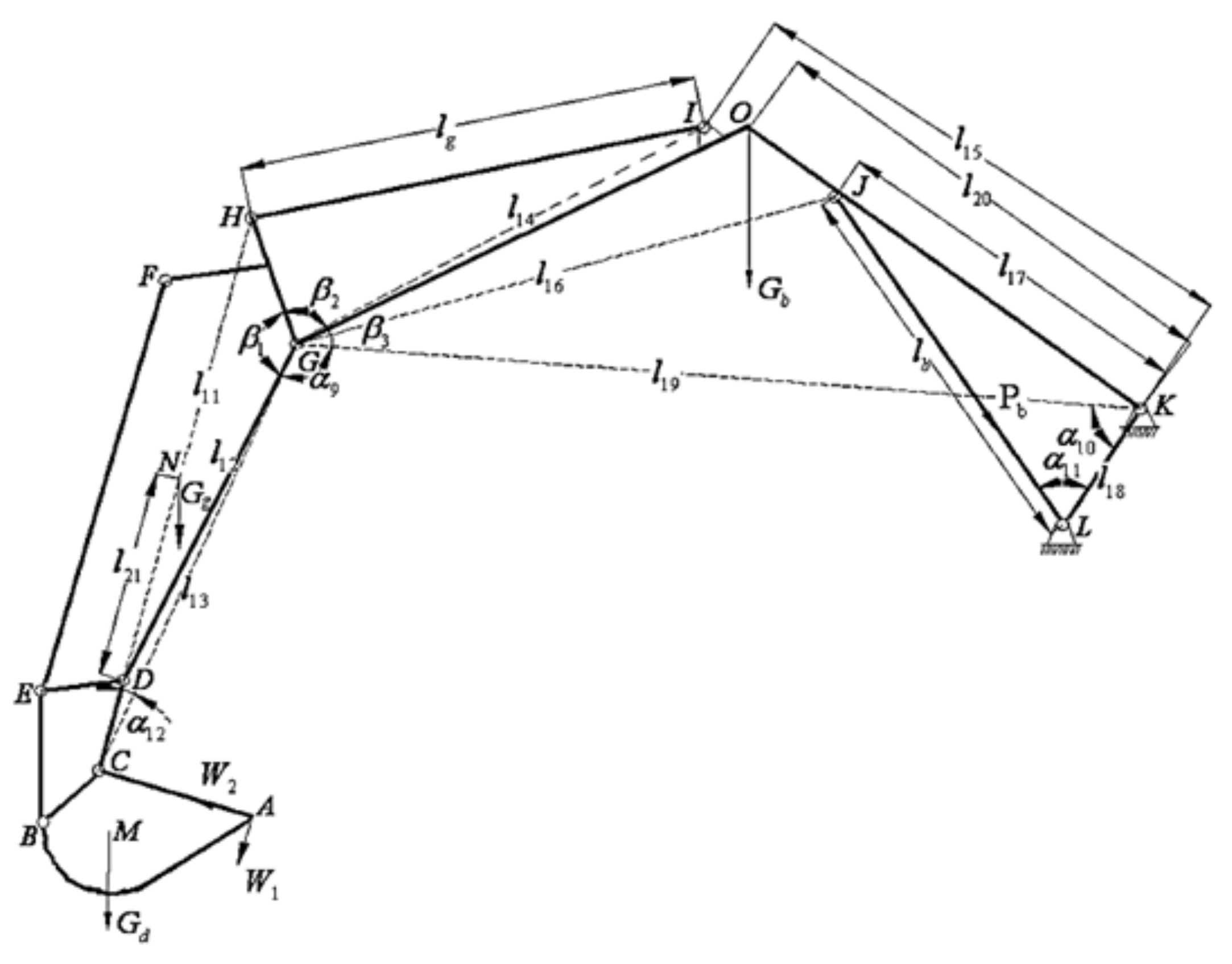
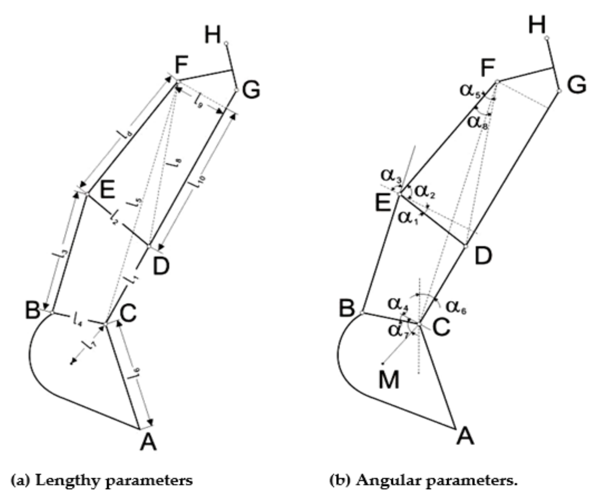
3.1. The Geometric Parameters of the Excavator Beam

The working beam of the hydraulic excavator consists of the bucket, the bucket arm, the swing boom, and 4 main cylinders. All parts are connected by pivots and driven by cylinders to complete the task of excavating. The schematic diagram of machinery and the geometric parameters of the working beam are illustrated in Figure 2. The forehead of the bucket arm is a 4 bars mechanism that is named linkage machinery. Its geometric model including the lengthy and angular parameters is illuminated as Figure 3. The implications of all alphabets are explained in the annotation table.

Through solving the triangles in the geometric model, all geometric parameters including angular parameters can be formulated by the lengthy parameters of the beam machinery. All lengthy parameters are constant parameters except the lengths of the cylinders. The fourth cylinder and the third one is symmetrically and synchronously assembled under both sides of the swing boom. For simplifying the machinery diagram, these two cylinders are represented by one variable of $l_b$ ($l_b$ is the length of the arm cylinder of the hydraulic excavator). Therefore, the geometric model of the beam machinery is a 3-freedom mechanism depending on the lengths of the 3 groups of main cylinders $l_d$, $l_{\mathrm{g}}$, $l_b$ ($l_d$ is the length of the bucket cylinder of the hydraulic excavator; $l_{\mathrm{g}}$ is the length of the bucket rod cylinder of the hydraulic excavator). The associated initial length of the cylinder rod is expressed as a variable $d_1, d_2, d_3$ (The three in turn are the initial length of the bucket cylinder, bucket rod cylinder and boom cylinder of the hydraulic excavator).

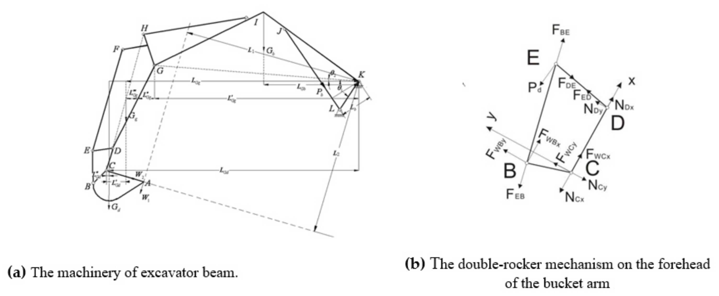
3.2. The Dynamic Machinery Model Driven by Thrust Forces of Hydraulic Cylinders

Many literatures estimated firstly the excavating resistant forces at the tooth tip of bucket depending on the mechanical properties of soils and stones for the machinery design [14]. The excavating resistant force is a special type of boundary condition of the dynamic model for the beam machinery. Therefore, it is critical to solving the dynamic model and shall be computed firstly. However, the theoretical estimations on the excavating resistant forces had excessive errors due to the uncertainty and diversity of the soils and stones. Further, the direct test for the excavating resistant forces is extremely difficult since it is impossible to install the sensors and strain gauges on the tooth tips of the bucket.

Therefore, this dynamic model of the beam machinery as Figure 4a is proposed to estimate the excavating resistant forces by using the thrust forces of cylinders since it is easier to accurately obtain the thrust forces of cylinders. The thrust force of the bucket cylinder is the product of the compressive stress and the section area of the cylinder rod. The compressive stress of the cylinder rod, as a type of simple unidirectional stress state, can be easily monitored in real-time while the excavator works. Subsequently, the supporting force at each pivot is obtained through plugging the excavating resistant forces into the model of beam machinery. When the thrust forces of cylinders are monitored in real-time, the time history of supporting force at each pivot is computed for the acquisition of the load spectra at pivots.

3.3. The Solutions of the Load Spectra at the Bucket Tooth Tip and Pivots

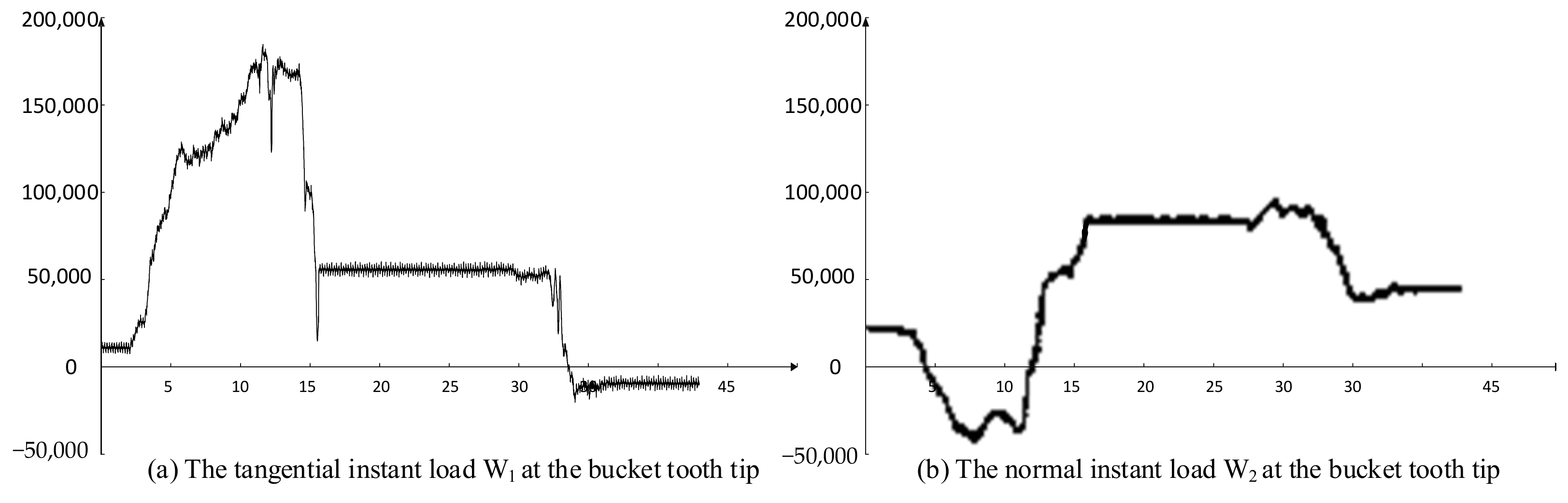
3.3.1. The Tangential Vector of Excavating Force W₁ at the Bucket Tooth Tip

The tangential vector of the excavating resistant force can be computed through analyzing the mechanical model of the double-rocker mechanism at the forehead of the bucket arm, as shown in Figure 4b. Assuming the double-rocker mechanism as the free body, the pivot C as the origin of coordinates, the direction of bucket arm as x-axis, and the direction perpendicular to bucket arm as y-axis, a local coordinate system is established on the bucket arm and the moment equilibrium equation of pivot C is established considering the gravity of bucket as the following:

$$W_1{l}_6=P_d{l}_{5}sin{\alpha }_5+N_{Dy}{l}_1+G_d{l}_{7}cos\left({\alpha }_4+{\alpha }_7-{\alpha }_6\right)$$

(1)

The equilibrium equations of the pivot B, C, D, and E in Figure 4b can be established as below:

$$\left\{\begin{array}{c}{F}_{wBx}=F_{EB}\mathit{sin}{\alpha }_3\\ F_{wBy}=F_{EB}\mathit{cos}{\alpha }_3\end{array}\right.$$

(2)

$$\left\{\begin{array}{c}{F}_{wcx}=N_{cx}\\ F_{wcy}=N_{cy}\end{array}\right.$$

(3)

$$\left\{\begin{array}{c}{F}_{ED}\mathit{cos}{\alpha }_1+N_{Dy}=0\\ F_{ED}\mathit{sin}{\alpha }_1+N_{Dx}=0\end{array}\right.$$

(4)

$$\left\{\begin{array}{c}{P}_d\mathit{cos}{\alpha }_2+F_{BE}\mathit{cos}{\alpha }_3=F_{DE}\mathit{cos}{\alpha }_1\\ P_d\mathit{sin}{\alpha }_2+F_{DE}\mathit{sin}{\alpha }_1=F_{BE}\mathit{sin}{\alpha }_3\end{array}\right.$$

(5)

Solving the equation set above, the tangential force of W₁ can be obtained as below:

$$W_1=\left[\frac{l_5}{l_6}\mathit{sin}{\alpha }_5-\frac{\mathit{sin}\left({\alpha }_2+{\alpha }_3\right)}{\mathit{sin}\left({\alpha }_3-{\alpha }_1\right)}\frac{l_1}{l_6}\mathit{cos}{\alpha }_1\right]{\sigma }_d{A}_d+G_d\frac{l_7}{l_6}\mathit{cos}\left({\alpha }_4+{\alpha }_7-{\alpha }_6\right)$$

(6)

3.3.2. The Normal Vector of Excavating Force W₂ at the Bucket Tooth Tip

Similarly, the normal vector of the excavating resistant force can be computed through analyzing the mechanical model of the whole machinery of the excavator beam, as shown in Figure 4a. Assuming the whole machinery as the free body, the moment equilibrium equation of the pivot K is established as following:

$$W_2{L}_2+W_1{L}_1=P_b{L}_b+\left(G_b{L}_{Gb}+G_g{L}_{Gg}+G_d{L}_{Gd}\right)$$

(7)

In which,

$$L_1=l_{19}\mathit{cos}\left[{\alpha }_9-\left({\alpha }_{12}+{\alpha }_4+{\alpha }_6-\frac{\pi }{2}\right)\right]-l_{13}\mathit{cos}\left({\alpha }_{12}+{\alpha }_4+{\alpha }_6-\frac{\pi }{2}\right)-l_6$$

(8)

$$L_2=l_{13}\mathit{sin}\left({\alpha }_{12}+{\alpha }_4+{\alpha }_6-\frac{\pi }{2}\right)+l_{19}\mathit{sin}\left[{\alpha }_9-\left({\alpha }_{12}+{\alpha }_4+{\alpha }_6-\frac{\pi }{2}\right)\right]$$

(9)

$$L_b=l_{18}\mathit{sin}{\alpha }_{11}$$

(10)

The arms of forces $L_{Gb}$, $L_{Gg}$, $L_{Gd}$ (The three in turn are the arm gravity, bucket rod gravity, bucket gravity to hinge point K moment arm) can be expressed by the geometric parameters of the beam machinery as shown in Figure 3.

$$L_{Gb}=l_{20}\mathit{cos}\left({\mathit{cos}}^{-1}\frac{l_{17}^2+l_{19}^2-l_{16}^2}{2l_{17}{l}_{19}}+{\alpha }_{10}-{\theta }_1\right)$$

(11)

$$L_{Gg}=L_{Gg}^{\prime }+L_{Gg}^{″}+L_{Gg}^{‴}$$

(12)

$$L_{Gd}=L_{Gg}+L_{Gd}^{\prime }-L_{Gd}^{″}$$

(13)

Through solving the triangles in the beam machinery, all geometric parameters including angular parameters in the equations listed above, can be formulated by the lengths of the cylinders and the machinery parts. It is easier to obtain the normal force of W₂ (W₂ is the normal force of the excavation force at the bucket tooth tip) as below.

3.3.3. The Solution of Load Spectra at Pivots

$$\begin{array}{c}{W}_2=\frac{P_b{l}_{18}\mathit{sin}{\alpha }_{11}-W_1\left\{l_{19}\mathit{cos}\left[{\alpha }_9-\left({\alpha }_{12}+{\alpha }_4+{\alpha }_6-\frac{\pi }{2}\right)\right]-l_{13}\mathit{cos}\left({\alpha }_{12}+{\alpha }_4+{\alpha }_6-\frac{\pi }{2}\right)-l_6\right\}}{\left\{l_{13}\mathit{sin}\left({\alpha }_{12}+{\alpha }_4+{\alpha }_6-\frac{\pi }{2}\right)+l_{19}\mathit{sin}\left[{\alpha }_9-\left({\alpha }_{12}+{\alpha }_4+{\alpha }_6-\frac{\pi }{2}\right)\right]\right\}}\\ +\frac{\left[G_b{l}_{20}\mathit{cos}\left({\mathit{cos}}^{-1}\frac{l_{17}^2+l_{19}^2-l_{16}^2}{2l_{17}{l}_{19}}+{\alpha }_{10}-{\theta }_1\right)+G_g\left(L_{Gg}^{\prime }+L_{Gg}^{″}+L_{Gg}^{‴}\right)+G_d\left(L_{Gg}+L_{Gd}^{″}-L_{Gd}^{\prime }\right)\right]}{\left\{l_{13}\mathit{sin}\left({\alpha }_{12}+{\alpha }_4+{\alpha }_6-\frac{\pi }{2}\right)+l_{19}\mathit{sin}\left[{\alpha }_9-\left({\alpha }_{12}+{\alpha }_4+{\alpha }_6-\frac{\pi }{2}\right)\right]\right\}}\end{array}$$

(14)

After being solved, the excavating forces at the bucket tooth tips are considered as the boundary conditions of the dynamic model of the beam machinery. Assuming the bucket as the free body, the force equilibrium equations is established while considering the gravity of the bucket as the following:

$$\left\{\begin{array}{c}{W}_2\mathit{cos}\left(\pi -{\theta }_3\right)+F_{Cx}=W_1\mathit{cos}\left({\theta }_3-\frac{1}{2}\pi \right)+F_{EB}\mathit{cos}{\gamma }_2+G_d\mathit{cos}{\alpha }_6\\ W_2\mathit{sin}\left(\pi -{\theta }_3\right)+W_1\mathit{sin}\left({\theta }_3-\frac{1}{2}\pi \right)+F_{Cy}=F_{EB}\mathit{sin}{\gamma }_2+G_d\mathit{sin}{\alpha }_6\end{array}\right.$$

(15)

Hence, depending on Equation (5), the supporting reaction forces at pivot C is obtained as:

$$\{\begin{array}{c}{F}_{Cx}=W_1\mathit{cos}\left({\theta }_3-\frac{1}{2}\pi \right)+P_d\frac{\mathit{cos}{\alpha }_1\mathit{sin}{\alpha }_2+\mathit{sin}{\alpha }_1\mathit{cos}{\alpha }_2}{\mathit{cos}{\alpha }_1\mathit{sin}{\alpha }_3-\mathit{sin}{\alpha }_1\mathit{cos}{\alpha }_3}\mathit{cos}{\gamma }_2+G_d\mathit{cos}{\alpha }_6-W_2\mathit{cos}\left(\pi -{\theta }_3\right)\\ F_{Cy}=P_d\frac{\mathit{cos}{\alpha }_1\mathit{sin}{\alpha }_2+\mathit{sin}{\alpha }_1\mathit{cos}{\alpha }_2}{\mathit{cos}{\alpha }_1\mathit{sin}{\alpha }_3-\mathit{sin}{\alpha }_1\mathit{cos}{\alpha }_3}\mathit{sin}{\gamma }_2+G_d\mathit{sin}{\alpha }_6-W_2\mathit{sin}\left(\pi -{\theta }_3\right)-W_1\mathit{sin}\left({\theta }_3-\frac{1}{2}\pi \right)\end{array}$$

(16)

Depending on Equations (2)–(5), the support reaction forces at pivot D is obtained as,

$$\left\{\begin{array}{c}{F}_{Dx}=-P_d\frac{\mathit{sin}\left({\alpha }_2+{\alpha }_3\right)}{\mathit{sin}\left({\alpha }_3-{\alpha }_1\right)}\mathit{sin}{\alpha }_1\\ F_{Dx}=-P_d\frac{\mathit{sin}\left({\alpha }_2+{\alpha }_3\right)}{\mathit{sin}\left({\alpha }_3-{\alpha }_1\right)}\mathit{cos}{\alpha }_1\end{array}\right.$$

(17)

Similarly, depending on Figure 3, the forces equilibrium equations of the bucket arm is obtained,

$$\left\{\begin{array}{c}{W}_2\mathit{cos}\left(\pi -{\theta }_3\right)+F_{Gx}=W_1\mathit{cos}\left({\theta }_3-\frac{1}{2}\pi \right)+G_d\mathit{cos}{\alpha }_6+G_g\mathit{cos}{\alpha }_6+P_g\mathit{cos}{\theta }_4\\ W_2\mathit{sin}\left(\pi -{\theta }_3\right)+W_1\mathit{sin}\left({\theta }_3-\frac{1}{2}\pi \right)+F_{Gy}+P_g\mathit{sin}{\theta }_4=G_d\mathit{sin}{\alpha }_6+G_g\mathit{sin}{\alpha }_6\end{array}\right.$$

(18)

Hence, the support reaction forces at pivot G is obtained as:

$$\left\{\begin{array}{c}{F}_{Gx}=W_1\mathit{cos}\left({\theta }_3-\frac{1}{2}\pi \right)+G_d\mathit{cos}{\alpha }_6+G_g\mathit{cos}{\alpha }_6+P_g\mathit{cos}{\theta }_4-W_2\mathit{cos}\left(\pi -{\theta }_3\right)\\ F_{Gy}=G_d\mathit{sin}{\alpha }_6+G_g\mathit{sin}{\alpha }_6-W_2\mathit{sin}\left(\pi -{\theta }_3\right)-W_1\mathit{sin}\left({\theta }_3-\frac{1}{2}\pi \right)-P_g\mathit{sin}{\theta }_4\end{array}\right.$$

(19)

Further, the forces at the pivots of I and J are presented as the following formulas according to the principle of a two-force rod. The force directions of the pivot I and J are along with the direction of the bucket arm cylinder HI and the boom cylinder JL.

$$F_I=P_g={\sigma }_g{A}_g$$

(20)

$$F_J=P_b={\sigma }_b{A}_b$$

(21)

In summary, all pivots on the excavator beam can be analyzed by the equilibrium equations of forces and moments according to Figure 4. All equilibrium equations can be finally indicated by only 6 independent variables of cylinder thrust forces of $P_d$, $P_g$, $P_b$ (The three in turn are the thrust of the bucket cylinder, the boom cylinder and the bucket rod cylinder that are measured by the test) and the corresponding cylinder lengths of $l_d$, $l_g$, $l_b$. These 6 independent variables are relevant to the working time $t$, therefore the load spectra at pivots in the time domain can be indicated by the general formula below,

$$\left\{\begin{array}{c}{F}_{PIVOTx}\left(t\right)=f_x\left[P_d\left(t\right),P_d\left(t\right), P_b\left(t\right), l_d\left(t\right), l_g\left(t\right), l_b\left(t\right)\right]\\ F_{PIVOTy}\left(t\right)=f_y\left[P_d\left(t\right),P_d\left(t\right), P_b\left(t\right), l_d\left(t\right), l_g\left(t\right), l_b\left(t\right)\right]\end{array}\right.$$

(22)

After the 6 independent variables tested or monitored in works in real-time are plugged into the formula set (22), the load spectra in the time domain can be computed for the further stimulation of the stress changes on the machinery parts.

4. The Stress Spectra and Frequency Spectra at Risk Nodes

4.1. The Stress Spectra by FEA Modeling

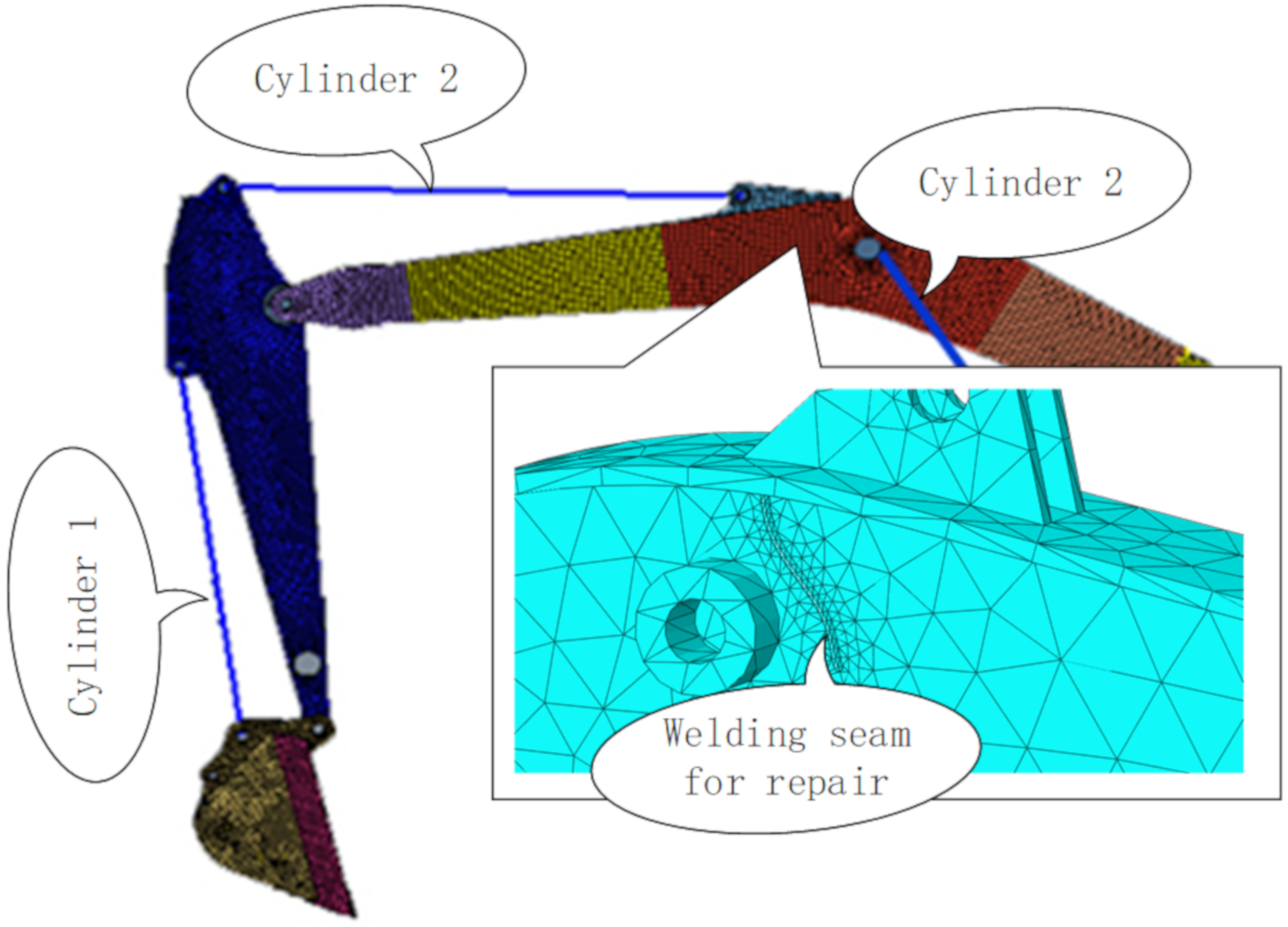
4.1.1. The FEA Model of the Remanufactured Beam Considering the Repaired Welding Joint

Furthermore, for obtaining the stress spectra at any node on the machinery, a FEA model is established by using the 3D modeling and meshing software. The load spectrum in the time domain obtained above is loaded at the given pivot as the boundary conditions of the FEA model and subsequently, the stress spectrum at any nodes on the machinery parts is computed. Since the lengthy dimensions of the whole excavating beam are much greater than the thickness, the meshes with four nodes shell elements are generated for the preprocessing. The kind of 2D shell meshes are drawn on the neutral layer that is extracted from the lengthy dimensions. The mesh nodes should align with each other through patching or linking the discrete faces with the 1D elements. The section properties of shell elements are defined depending on the real thicknesses and the materials of the steel plates used on the excavating beam.

The preprocessing model is illustrated in Figure 5. The various colors represent various thicknesses of the shell elements with the various section properties. That means the excavating beam consists of various steel plates with various thicknesses. Considering the condition of remanufacturing, the FEA model for repair welding boom was created and fatigue life prediction would be made in this paper. Due to the same working condition as above, the modeling process and mash process were provided. Firstly, the 3D model of the boom was created by writing code and the weld for the 3D model was created on weld design interface. And the Fillet weld as the welding model was selected. And then the model will be imported to finite element software for analysis. The FEA model of the repair welding arm is shown in Figure 5. Finally, considering the special shape, a regular tetrahedral mesh was created at unimportant positions, and then the welding area has partially meshed. The mud model of the repair welding arm is shown in Figure 5.

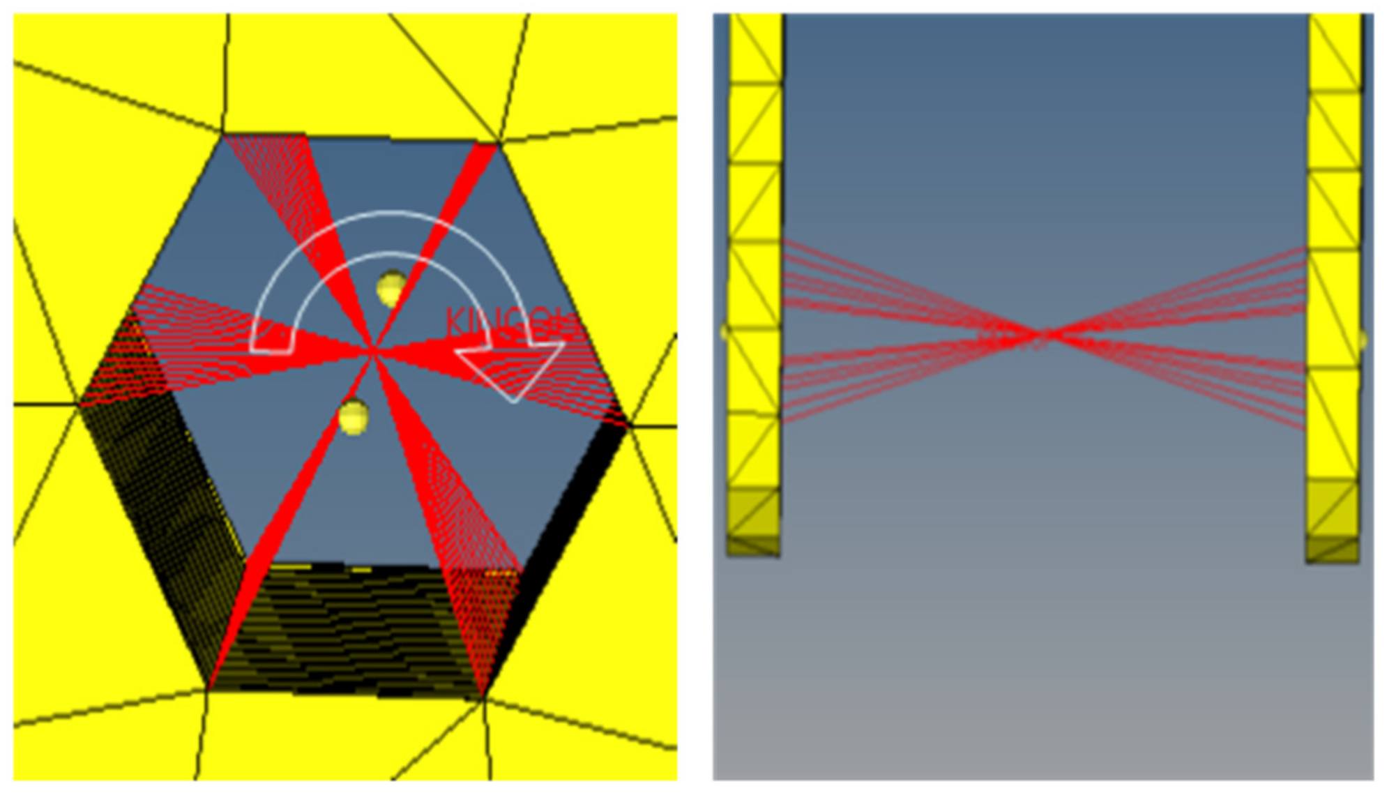
4.1.2. The Boundary Condition Setting and the Loading at Pivots

Since the transient dynamic FEA method is established for the acquisition of stress spectra, the analytical step is configured with a time cycle. Those cycles and periods keep correspondence with the sampling cycle and the period of the test. Considering the mechanism and hydraulic damps, the Rayleigh damping coefficient is configured from 1 to 10 and the mass array coefficient of Rayleigh damp as 3, and the stiffness array coefficient as 0. All pivots linking the parts with each other and the framework is defined as a fixed constraint only 1 DOF (Degree of Freedom) of the rotation on the pivot axis is released. The constraint model of the pivot is proposed as Figure 6.

While the bucket arm and the swing beam are separated as the free bodies, the thrust forces of cylinders and the supporting reaction forces at pivots will be loaded as the boundary conditions of the machinery parts. The load amplitude is defined by the load spectrum computed by the machinery dynamic model mentioned above. The load spectrum in the time domain is loaded at the given pivot on the arm and beam parts as the boundary conditions of the FEA model. By using the standard solver, the stress and the corresponding variation at each node on the beam parts is computed at various moment in the sampling cycle. Hence the stress spectrum at any given node, usually the key node on the risk section of the part, can be acquired in the time domain.

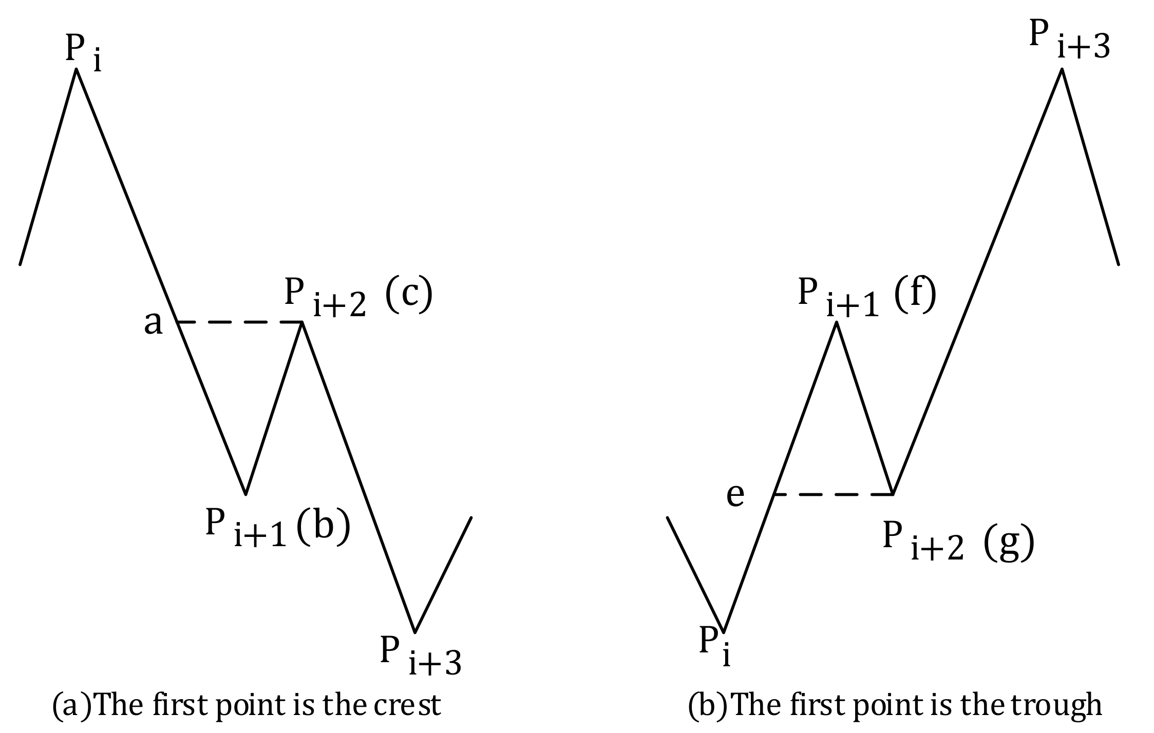
4.2. The Frequency Spectra by RFC Method

Depending on the stress spectrum at the risk nodes, the frequency spectrum of the stress amplitude and mean can be obtained using the RFC (Rain Flow Counting) method. The frequency spectrum is the hypothesis for the estimation of the fatigue damage by considering the structure. The RFC method with double variables is usually used in mechanical engineering. It counts the frequency number relevant to the variable of the stress amplitude and the stress mean. It exactly reflects the fatigue characteristics of the machinery under the actions of dynamic and static strength [15]. Therefore, the RFC method is usually used to process the stress spectrum and obtain the frequency spectrum as the data input for the DFR (Detailed Fatigue Rating) model.

The four-points RFC method obtains the frequency number via cycling counting every four peaks and valleys of the stress spectrum. Its principle can be demonstrated as the Figure 7.

That means a cycling count consists of four neighboring peaks and valleys if satisfying the rules below,

$${\mathrm{P}}_{\mathrm{i}}\ge {\mathrm{P}}_{\mathrm{i}+2} \mathrm{and} {\mathrm{P}}_{\mathrm{i}+1}\ge {\mathrm{P}}_{\mathrm{i}+3}\hspace{1em}\hspace{1em}\hspace{1em}(\mathrm{i} = 1, 2\dots )$$

$$\mathrm{or} {\mathrm{P}}_{\mathrm{i}}\le {\mathrm{P}}_{\mathrm{i}+2} \mathrm{and} {\mathrm{P}}_{\mathrm{i}+1}\le {\mathrm{P}}_{\mathrm{i}+3}\hspace{1em}\hspace{1em}(\mathrm{i} = 1, 2\dots )$$

Meanwhile, the stress amplitude in the counting cycle is ${\mathrm{S}}_{\mathrm{a}}=\left|{\mathrm{P}}_{\mathrm{i}+1}-{\mathrm{P}}_{\mathrm{i}+2}\right|/2$. The stress mean in the counting cycle is ${\mathrm{S}}_{\mathrm{m}}=\left|{\mathrm{P}}_{\mathrm{i}+1}+{\mathrm{P}}_{\mathrm{i}+2}\right|/2$. After recording the stress amplitude and mean, the peak value ${\mathrm{P}}_{\mathrm{i}}$ and the valley value ${\mathrm{P}}_{\mathrm{i}+1}$ are extracted from the stress spectrum. Cycling the counting step based on the rules above, the stress spectrum in the time domain is transferred to the discrete number of cycles relevant to the stress amplitude and mean. Any time-domain signal can be transferred to a matrix of rain flow with residues, which also can be recovered to the continuous time-domain signal. Consequently, the frequency spectrum at any node in the domains of stress amplitude and mean can be effectively obtained via processing the stress spectrum in the time domain with the RFC method.

5. The Fatigue Life Prediction Based on the DFR Model

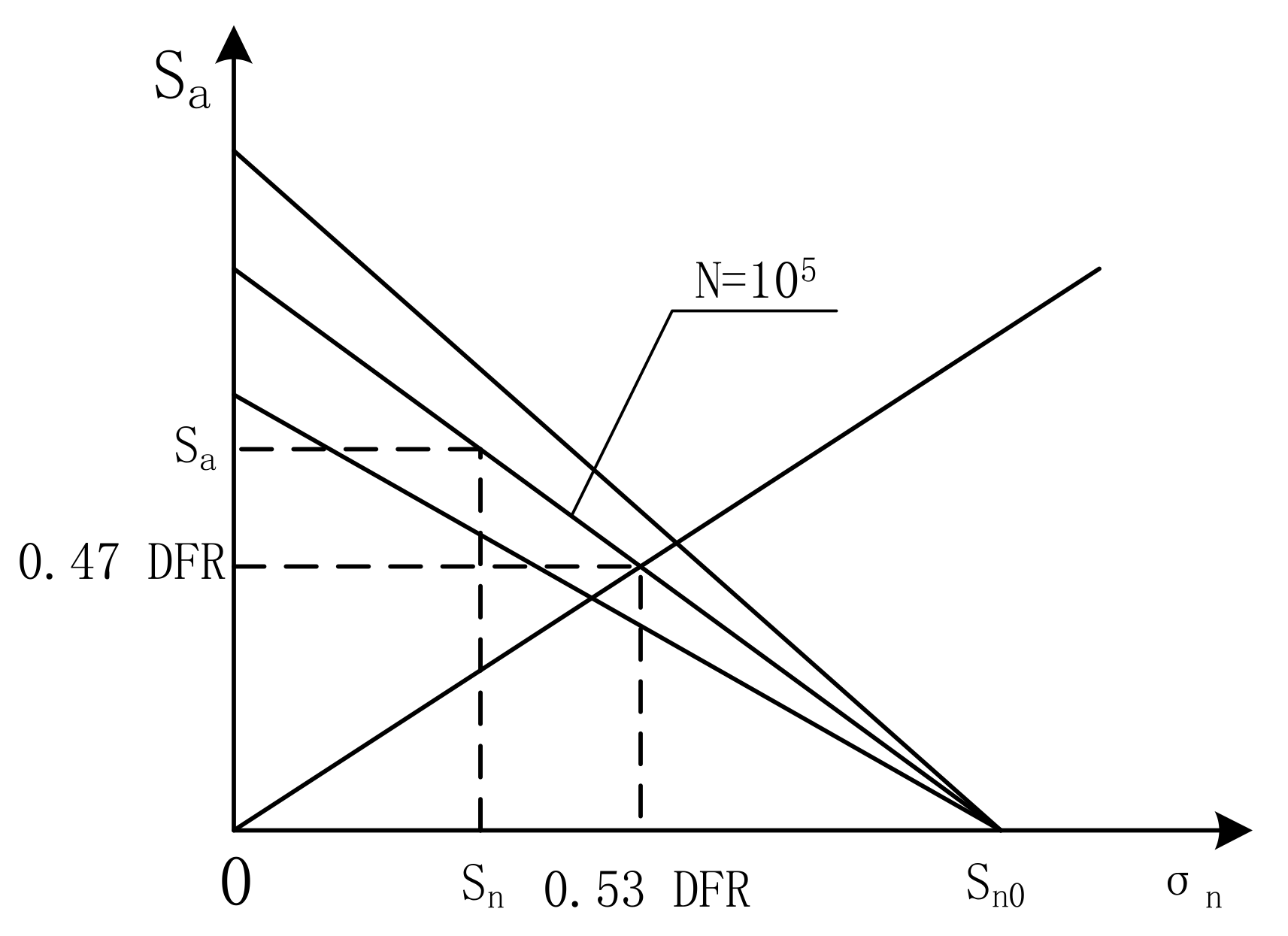
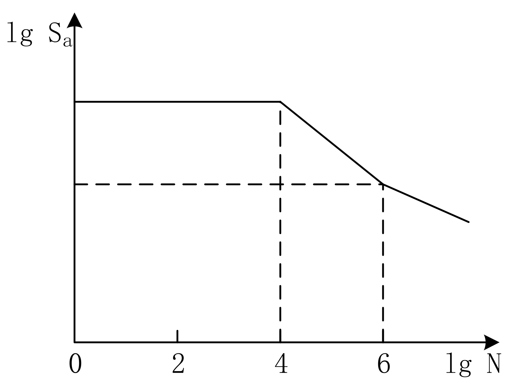
5.1. The Corrected S-N Curve by the DFR Method Depending on the Beam Structure

The S-N curve is generally conservative while estimating the mid-long fatigue life under the extremely lower stress. The S-N curve only indicates the real fatigue life (the number of stress cycles before the fatigue fracture) in the bench test under the symmetric cycling stress. That means the stress mean is nearly zero while the fatigue life of the given material is measured on the test bench. Therefore, it is hard for the S-N curve to indicate the characteristics of the fatigue while the stress mean is non-zero and the stress amplitude is not large. For better indicating the real fatigue property under various stress amplitudes and means, the S-N curve needs to be corrected by the DFR (Detailed Fatigue Rating) model.

The DFR model is a set of theoretic equations that can be used to correct the S-N curve depending on the experimental data from the bench test. DFR hypothesizes that the fatigue life obeys the two-parameter Weibull distribution while the stress amplitude S_a and fatigue life N vary with the inverse relationship in the long-life regime (N > 10⁴) [16]. The equivalent life curves are straight lines and all of them intersect with the abscissa axis at S_m0 (material parameter) in the long-life regime. Besides, the fatigue damage obeys the Miner accumulated fatigue damage rule.

The longevity region is the life interval which distributed like Weibull with the cycle times between 10⁴–10⁶ [16]. According to the DFR method, the linear relation between cycle times N and stress S_a is,

$$\mathrm{lgN}=\mathrm{A}+\mathrm{Blg}{S}_a$$

(23)

in which A is the material parameter and the B are the constants for the S-N slope in the double logarithm coordinate. Depending on the structure of the remanufactured beam, when life N = 10⁵, S_max = DFR, S_a = 0.47DFR, S_m = 0.53DFR. Substituting N =10⁵ into the Equation (23), there is

$$\mathrm{lgN}=\lg \frac{{10}^5}{{\left(0.47\mathrm{DFR}\right)}^B}+\lg {\left(S_{aD}\right)}^B$$

(24)

in which, $S_{aD}$ is the stress amplitude on the curve of equivalent fatigue life while the mean stress S_m = 0.53DFR as shown in Figure 8.

$$S_{aD}=\frac{S_{mo}-0.53\mathrm{DFR}}{S_{mo}-S_m}{S}_a$$

(25)

Plugging the Equation (25) into (24), the structure expression under the long life of the S-N curve is established like

$$\mathrm{lgN}=\lg \frac{{10}^5}{{\left(0.47\mathrm{DFR}\right)}^B}+\lg {\left(\frac{S_{mo}-0.53\mathrm{DFR}}{S_{mo}-S_m}{S}_a\right)}^B$$

(26)

Long-life area refers to the characteristics of life which is more than the number of cycle life span [17]. Assuming N to be constant, the curve is linear and the following Equation (27) is valid in the long life interval.

$$\mathrm{lgN}= \mathrm{A}\prime + \mathrm{B}\prime \lg S_a$$

(27)

By the statistical analysis on cycle times, the S-N curve slope is $B^{\prime }$= 5.68 under the condition of N $\ge {10}^6$ depending on the reference [18]. When plugging N = 10⁶ into (26), there is

$$S_a\left[{10}^6\right]=\frac{0.47\left(S_{mo}-S_m\right)\mathrm{DFR}}{S_{mo}-0.53\mathrm{DFR}}{S}^{-1}$$

(28)

In which, $\mathrm{S}={10}^{-\frac{1}{B}}$ is the slope of the S-N curve in a long-life regime.

Plugging N = 10⁶ into the Equation (27), the following Equation (29) is obtained.

$$A^{\prime }=\lg {10}^6-B^{\prime }\lg S_a\left[{10}^6\right]$$

(29)

Solving the Equation (27) with (28) and (29), the structure of S-N curve expression under N $\ge {10}^6$ long life is established as the equation (30).

$$\mathrm{lgN}=\lg \left\{{10}^6{\left[\frac{\left(S_{mo}-0.53\mathrm{DFR}\right)S_a}{0.47\mathrm{DFR}\left(S_{mo}-S_m\right)}\right]}^{B^{\prime }}*S^{B^{\prime }}\right\}$$

(30)

5.2. The Fatigue Life Prediction by the Miner Rule on the FDA Model

The fatigue life of the beam structure is estimated based on the S-N curve of the excavator beam and Miner linear fatigue criterion. According to the Miner criterion, when the damage cumulative value reaches 1, the structure won’t work. This article will rule the Miner correction based on the FDA model as follows:

$$N{\displaystyle \sum }_{i=1}^n\frac{n_i}{N_i}=a$$

(31)

Among them, n is the level of the stress spectrum.$n_i$ is the frequency times of the cyclic stress at a stress level during a working cycle. $N_i$ is the number of cycles at a stress level. $N$ is the total number of cycles at all stress levels before the failure of the remanufacturing beam.

The stress amplitude $S_a$ at a level, the mean stress $S_m$ and the frequency times $n_i$ relevant to the stress amplitude and the mean stress can be counted by RFC method depending on the stress spectra at crisis nodes. Besides, the circles $N_i$ at a stress level can be computed out via Equations (26) and (27). Through putting the $N_i$ and $n_i$ into Equation (31), the total working cycles N before the failure of the remanufacturing beam can be computed. Further depending on the working hours per day, the working days per year, and the sampling time of all load spectra, the fatigue life at each node on the remanufactured beam is estimated consequently.

6. Case Study on the Remanufactured Excavator Beam

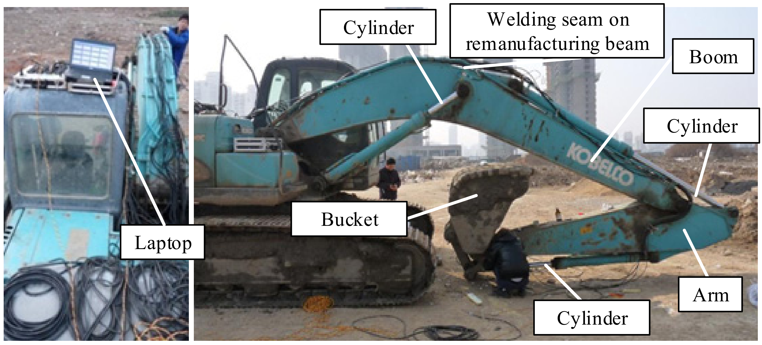
6.1. The Working Conditions of the Remanufactured Excavator Beam

The field test was conducted on the Kobelco SK210LC-8 excavator (This equipment is purchased in Wuhan from Hubei Jiushengxiang Machinery Equipment Co., Ltd., Wuhan, China) made in Japan, as shown in Figure 9. Assuming that the piston rod of the oil cylinder is only subjected to unidirectional stress, the stress history of the 3 main oil cylinders is measured while fixing the bucket and the arm, only moving the boom to excavate the soil ground. In this figure, the x coordinate axis represents the number of sampling points during the sampling time 43 s with the sampling frequency 256 Hz. The y-axis represents the unidirectional stress in MPa. The stress history of the 3 groups of main cylinders is illustrated in Figure 10a. Meanwhile, the displacements of the piston rods of the main cylinders are measured and recorded by the wire displacement sensors. Furthermore, Figure 10b is obtained by fitting the displacement data of the main cylinders. The cross-sectional area of the piston rod of the main cylinders is respectively 5176 mm², 7166 mm², 2 × 5760 mm². Subsequently, the load history of the cylinders is computed through the unidirectional stress times the sectional area of the piston rod of the oil cylinders. Meanwhile, the changing force arms in the beam structure are computed depending on the displacement history of the cylinder rods. Both the histories of loads and displacements of the main cylinders are the key to the solutions of the forces on the bucket tooth tip and the beam pivots.

The measuring instrument is ASMC1-9 dynamic strain gauge developed by Jinan Sigma Co., Ltd., Jinan, Shandong. It has 9 channels and the strain measuring range is ±60,000 με with high accuracy and a variety of group bridge methods. Data from equipment instruction manual.

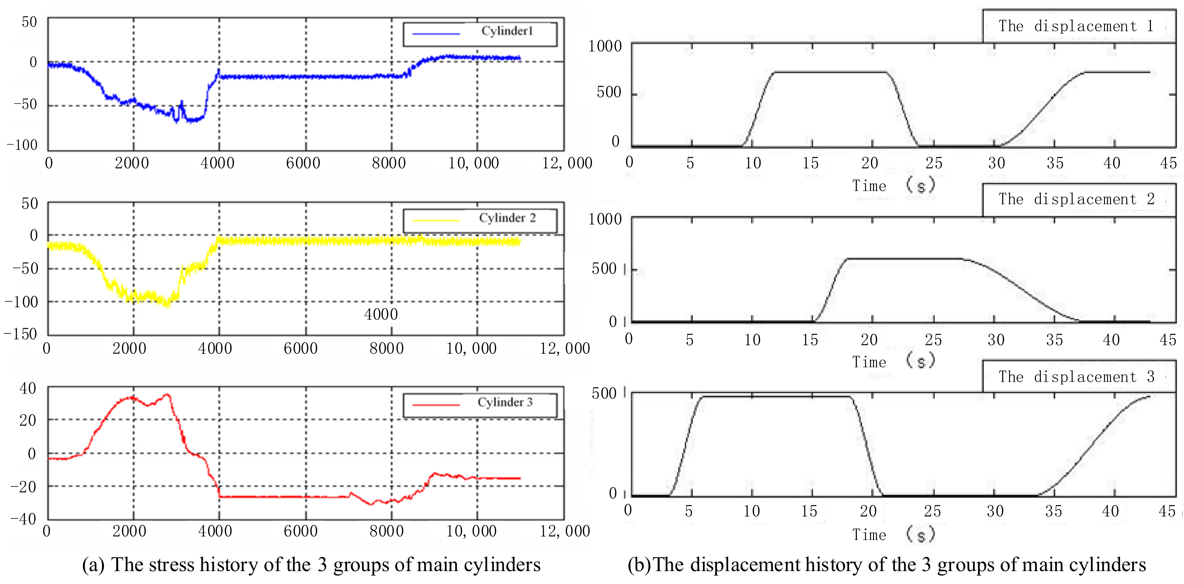
6.2. The Load Spectra of the Excavating Force Computed by the Dynamic Machinery Model

The tangential force W₁ and the normal force W₂ on the bucket tooth tip in the sampling cycles can be acquired via solving the dynamic machinery model depending on the Equations (6) and (14). The load spectra on the bucket tooth tip is computed and plotted out in Figure 11.

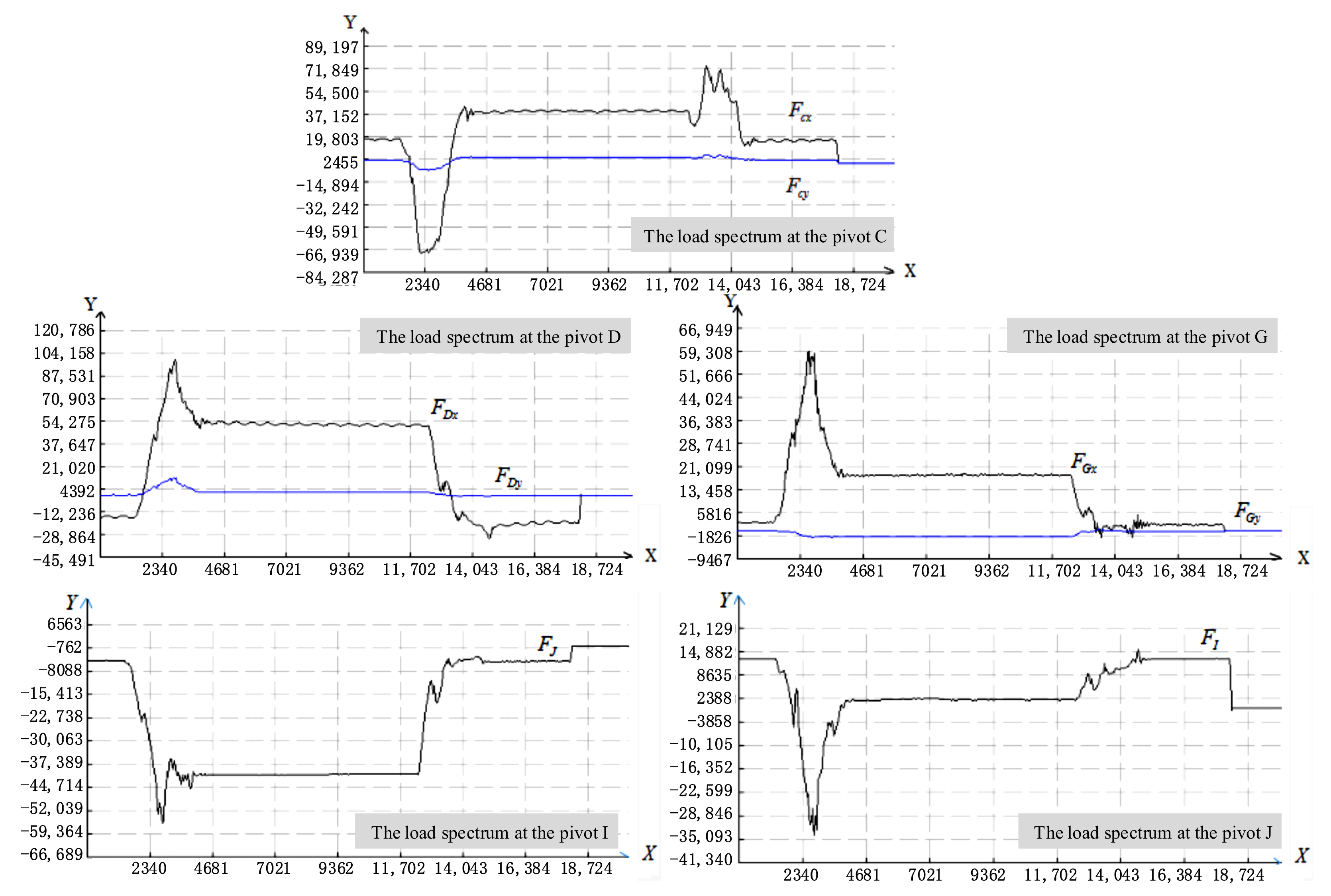
6.3. The Load Spectra of the Key Nodes on the Remanufactured Beam

Mechanism dynamics is the theoretical basis of modern machinery which is applied to analyze the relationship between the stress while working and the mechanical motion of machinery. By force analysis on each component of the working beam, the working load of bucket tooth tip and bucket cylinder, and the thrust of bucket arm cylinder and boom cylinder piston rods are computed relying on the working time. The computational formulas about the changing of normal and tangential working load on each pivot are deduced based on analyzing geometrical parameters of working devices. This paper sets an example on the working load of the bucket tooth tip and applies the deduced computational formulas to study its mechanism dynamics. As shown in Figure 12, the load spectra of 5 key pivots are recorded.

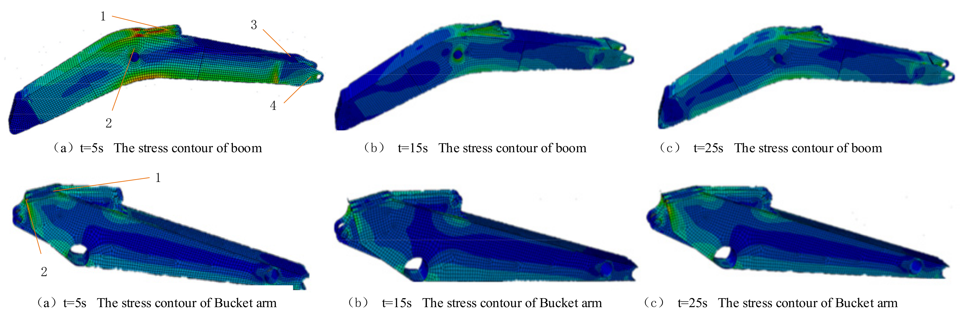
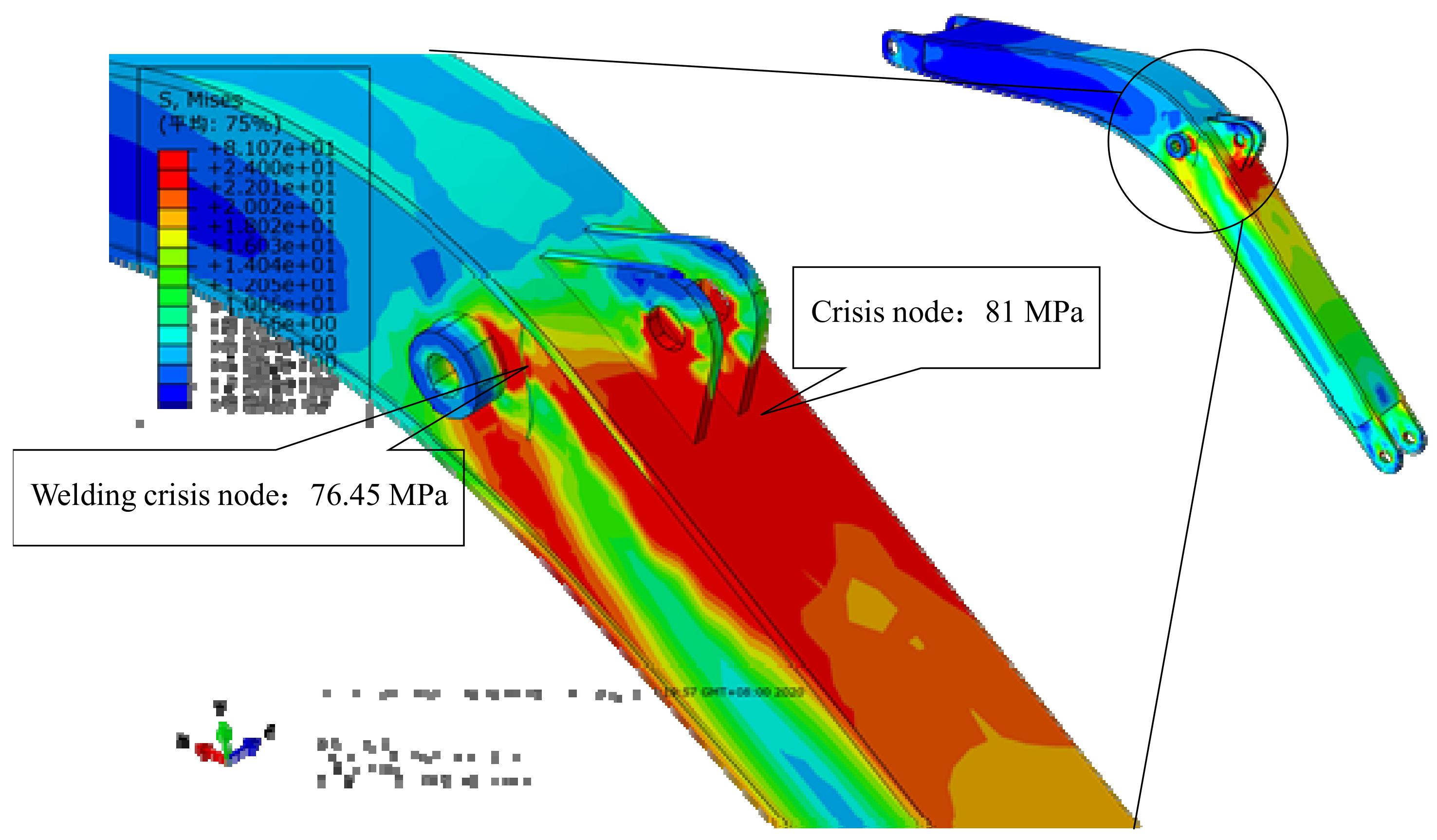
6.4. The Stress Contours on the Boom and Arm

Various operating conditions of hydraulic excavator are consisted of the movement among boom cylinder, bucket arm cylinder and bucket cylinder. The main load on it comes from axial force and bending moment. When the bucket arm is excavating, the dangerous section probably appears on the boom because of the maximum arm of force that the bucket arm cylinder put on it. Therefore, the static stress analysis and fatigue life study on working devices have proceeded under the digging working condition in this paper.

Firstly, a FEA model of the excavator beam is established through generating the meshes with 4-node shell elements since the axial dimensions of the beam are much broader than the lateral dimensions. The thickness of shell elements is consistent with the real dimensions of the beam. The thickness of the steel plate is listed in

Table 1. The thickness of the steel plate.

	Thickness	Cover Plate/mm	Side Plate/mm
Part
Beam		12/12	14/14
Arm		14/14	14/14
Bucket		20	20/20

. Besides, the material performances are indicated by the parameters in

Table 2. Material parameters of the excavator beam.

Material	Modulus of Elasticity/MPa	Poisson’s Ratio	Density/(t·mm−3)
16Mn	2.06 × 105	0.3	7.85 × 10−9

. Eventually, all load spectra at pivots are applied to the FEA model according to the hinged constraints. The dynamic stresses contours on the working beam during the sampling cycle is simulated as shown in Figure 13.

It is apparent seeing from the FEA model that the higher stress regions are located on node 1, node 2. At the moment of 5 s, the maximum stress is 75 MPa located on node 2 and the stress of node 4 on the bucket arm ear plate is around 56 MPa. Other regions work under lower stress so that their fatigue life is longer than the four nodes. According to Figure 13, the regions on the boom and the arm under higher stresses can be confirmed at various moments. Considering the random alternating load while working, 4 nodes on the boom and 2 on the arm are more likely to suffer fatigue failure under an excavating cycle.

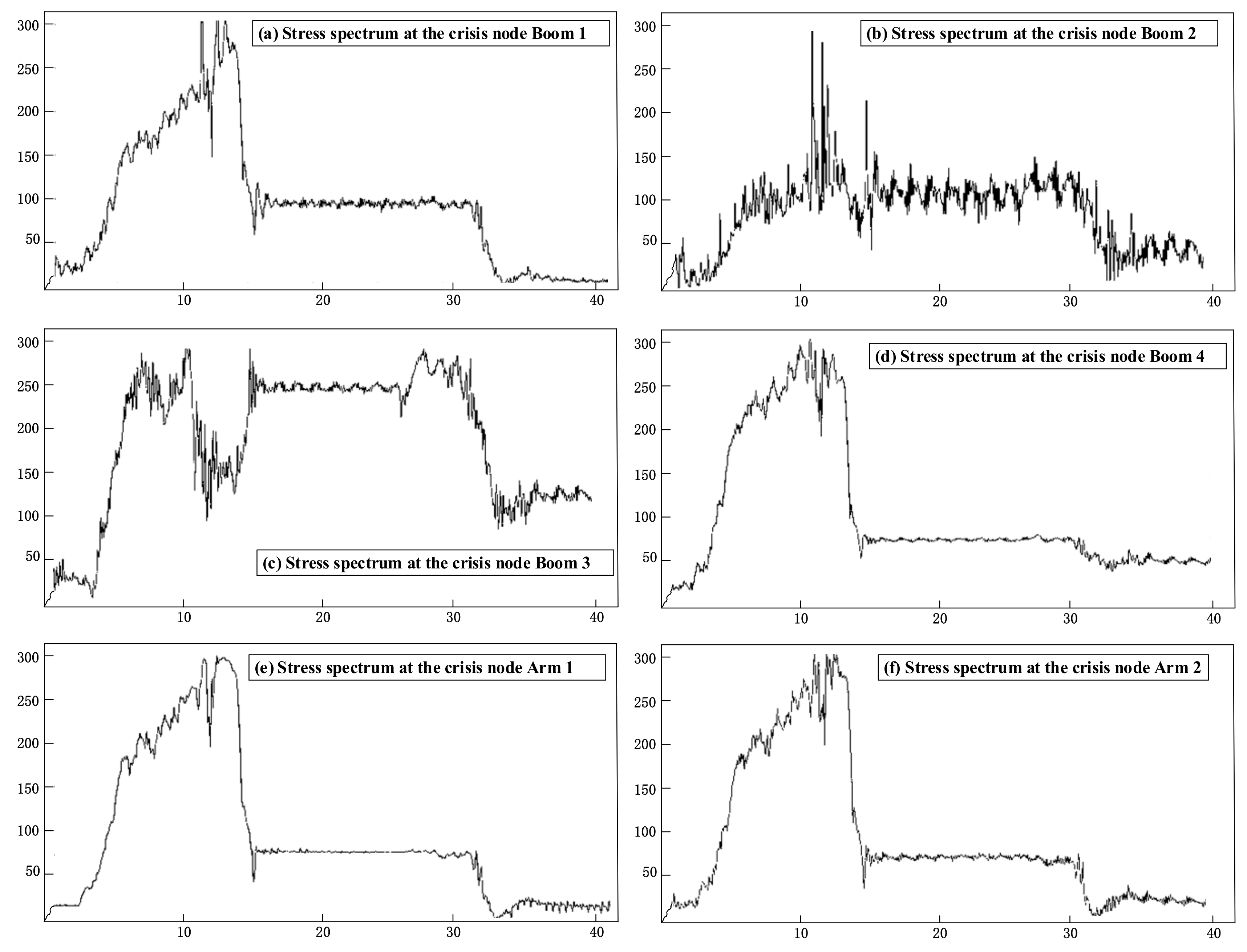
6.5. The Stress Spectra at the Key Nodes on the Boom and the Arm

Depending on the dynamic analytical results shown in Figure 13, it can be seen that the boom is mainly affected by the bending moment and the axial force. They cause the stress on the upper and lower cover plates is greater than that of both sides of beam plates. Meanwhile the structural shape of the boom at the reaming hole of the cylinder changes, which is prone to form the stress concentration around the reaming hole, as shown in Figure 13b.

The ear plate and the front flapper on the boom are in contact with the bucket cylinder and the bucket respectively. The external loads are usually applied on the contact points to form the high-stress areas, as shown in Figure 13a–c. Therefore, the beam safety and reliability must compute the fatigue life of the high-stress areas on the boom under the action of random external loads.4 nodes in the high-stress areas are selected as indicated in Figure 13a and their Element IDs in the FEA model are 45416/45473/46873/46895 respectively. The stress spectra at the 4 crisis nodes are output in Figure 14a–d, in which the x coordinate axis represents the sampling time and the coordinate axis represents the Mises stress at the crisis nodes.

Similarly, depending on the FEA data in Figure 13, it is apparent to find higher stress concentration exists in the boundary area at the reaming hole connecting the ear plate on the bucket arm to the boom. Therefore, the fatigue life at the bucket ear plate and the reaming hole needs to be computed for providing the maintenance reference and enhancing the reliability of the arm.2 crisis nodes in the high-stress area on the arm are selected with the element IDs 13556/18665. The stress spectra are output as shown in Figure 14e–f. Also, the x coordinate axis represents the sampling time and the coordinate axis represents the Mises stress at the crisis nodes.

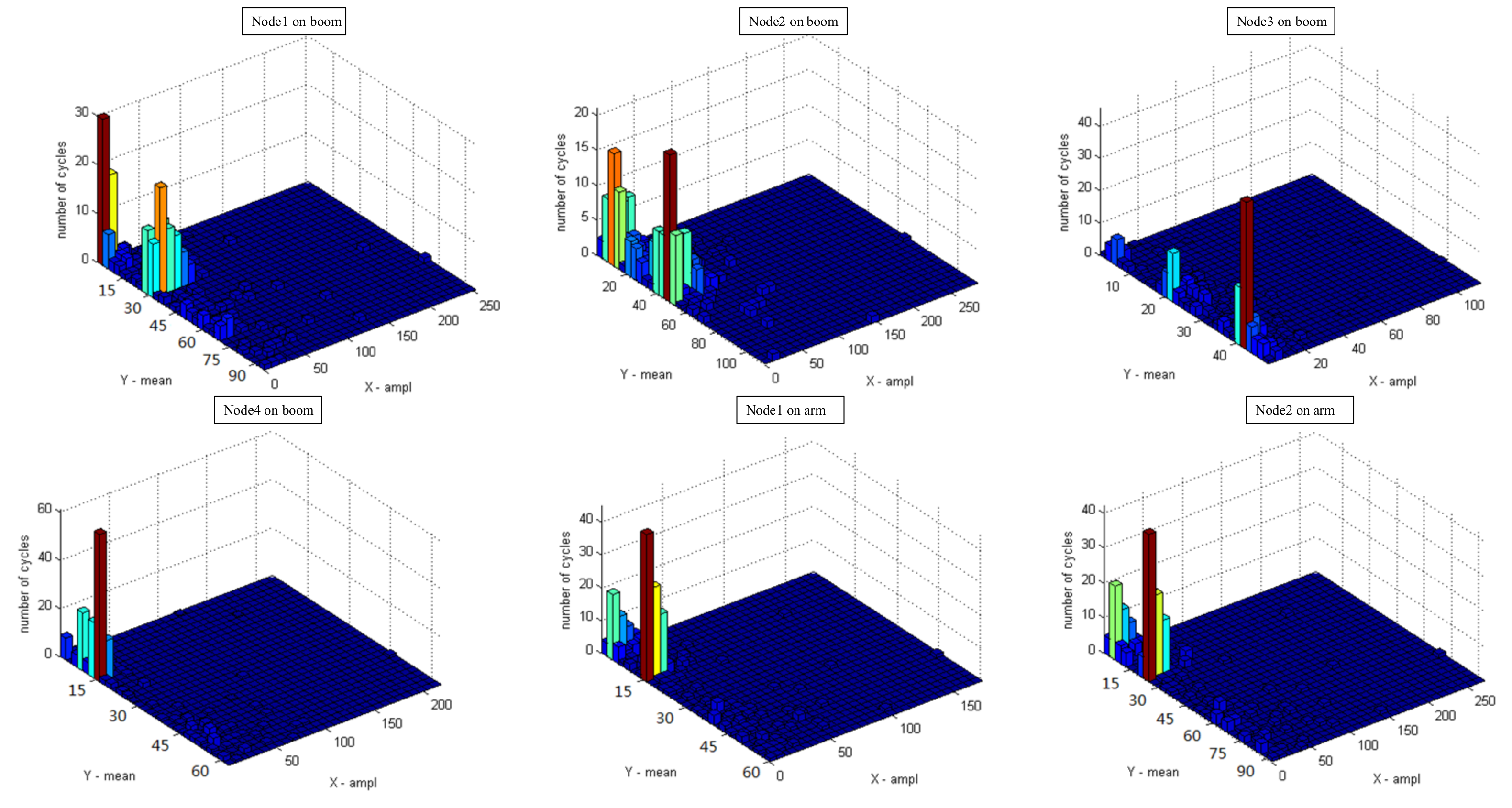
6.6. The Frequency Spectra at the Crisis Nodes on the Boom and the Arm

The dual-parameter rain flow counting (RFC) method counts the frequency times of real stress on various levels depending on the parameters of amplitude and mean stress. Using the RFC method can compute the entire frequency spectra through counting the typical pieces of the stress spectra and finally integrating them. In the high-stress area on the boom and the arm, the frequency spectra at the crisis nodes is acquired by counting and compiling the stress spectra with the RFC method, as shown in Figure 15. In the RFC diagram, the x-axis is the amplitude of the cyclic stress at the crisis node, the y axis stands for the mean of cyclic stress, and the z-axis represents the frequency times of cyclic stress at various stress levels at the crisis node. The RFC diagram shows the relations between the frequency times, the amplitude of stress, and the mean stress at the crisis nodes during a typical excavating cycle. In this case, the typical excavating cycle lasts a sampling cycle of only 43 s. Depending on the RFC data, it is apparent to find that the cycling stress applied on the beam is much lower than the yield strength of the 16Mn. That means the structural failure of the remanufactured beam also results from the accumulations of fatigue damages of the structure. However, the correction of the S-N curve needs to have proceeded so that it can indicate the unique fatigue properties of the remanufacturing machinery with a welding joint in a long-life regime.

6.7. The Corrected S-N Curve

The local material properties affected by the remanufacturing process need to be illustrated for the fatigue life prediction on the remanufacturing parts. Figure 16 shows the stress contour of the remanufactured excavator boom. The Mises stress at the crisis node on the welding seam is used to correct the S-N curve of 16 Mn steel affected by the welding heat around the seam. The thermal effects on the welding seam change the material properties and further change the S-N curve of the remanufactured material. This principle is used to calculate the DFR and further the fatigue life of the remanufactured excavator beam. It can be seen from Figure 16 that the Mises stress at the welding crisis node is 76.45 MPa.

Through the fatigue test, the DFR value of the remanufactured boom is decided. The material of the working beam is 16Mn low alloy steel.

Table 3. The fatigue life test on the remanufactured 16Mn.

Sa/MPa	${\mathit{S}}_{\mathit{T}}$	${\mathit{S}}_{\mathit{R}}$	${\mathit{S}}_{\mathit{C}}$	N
35	1.3	3.2	1.175	212,573,025
75	1.3	3.2	1.175	2,537,428
125	1.3	3.2	1.175	612,350
175	1.3	3.2	1.175	205,692

illustrates the fatigue test datum of several specimens of 16Mn with remanufactured welding seams. The fatigue life obeys the Weibull distribution therefore the shape parameter of the welding seam takes 3 as shown in

Table 4. The shape parameter of the welding seam.

Material	Aluminum Alloy	Titanium Alloy	Strength of Steel ${\mathit{\sigma }}_{\mathit{b}}\le$1655 MPa	High Strength Steel ${\mathit{\sigma }}_{\mathit{b}}>$1655 MPa
$\mathsf{\alpha }$	4.0	3.0	3.0	2.2

through looking up to the Weibull distribution [19].

In Table 4, S_T is the coefficient of test specimen, S_R is the reliability coefficient, S_C is the confidence coefficient. β is the characteristic life of the remanufactured welding material with Weibull distribution. There is

$$\beta ={\left[\frac{1}{n}{\displaystyle \sum }_{i=1}^n{N}_i^{\alpha }\right]}^{\frac{1}{\alpha }}$$

(32)

While the confidence coefficient of fatigue life of the remanufactured 16Mn at 95% reliability is N_95/95, there is

$$N_{95/95}=\beta /\left(S_T{S}_R{S}_C\right)$$

(33)

And the DFR value is calculated by the following Equation (34)

$$\left\{\begin{array}{l}{\mathrm{DFR}}_{base}=\frac{S_{mo}\left(1-R\right)}{0.94\frac{S_{mo}}{{\sigma }_{max}\left(0.47X-0.53\right)\left(0.47X+0.53\right)}}\\ X=S^{-1}{\left(\frac{N}{{10}^6}\right)}^{\frac{1}{B^{\prime }}}\\ \mathrm{DFR}={\mathrm{DFR}}_{base}*R_C\end{array}\right.$$

(34)

In which, R is the stress ratio of the test load, R = 0.06. σ_max is the calculated maximum load. R_C is the fatigue rating factor, and R_C = 1.4. X is the correction factor in the following Equation (34). According to the material properties, B = −3.92, S_m0 = 930 MPa, and the calculated values of other parameters are shown in

Table 5. Relevant Parameters Calculated Results.

Life	${\mathit{N}}_{95/95}$	B	${\mathit{S}}_{\mathit{m}\mathit{o}}$	${\mathbf{DFR}}_{\mathit{b}\mathit{a}\mathit{s}\mathit{e}}$	$\mathbf{DFR}$/MPa	$\mathit{X}$
6.875 × 105	1.4 × 105	−3.92	930	189.2	285	0.92

.

According to Equations (26) and (27), the corrected S-N curve of the remanufactured welding material is shown in Figure 17. Subsequently, the number of cycles at the stress level $i$ is decided by Equations (35) and (36) as shown below.

$${\mathrm{lgN}}_i=13.3376-3.92\lg \frac{778.95S_a}{930-S_m}(S_a>76.45 \mathrm{MPa})$$

(35)

$${\mathrm{lgN}}_i=4.5501-5.68\lg \frac{778.95S_a}{133.95\left(930-S_m\right)}(S_a\le 76.45 \mathrm{MPa})$$

(36)

6.8. The Fatigue Life Prediction on the Remanufactured Excavator Beam

In this case, the stress at crisis nodes is divided into 8 levels depending on the ratio of the amplitude to the mean. The stress amplitude $S_a$, the mean stress $S_m$ and the frequency times $n_i$ at a stress level at the crisis nodes on the beam during a working cycle are computed by RFC, depending on the stress spectra at the corresponding nodes. Subsequently, the amplitude S_a and the mean stress S_m are substituted into Equations (35) and (36) to calculate the number of cycles N_i at each stress level. The computed cycles on stress levels at crisis nodes depending on the stress frequency spectra and the corrected S-N curve of the remanufactured welding material are listed in

Table 6. Computed cycles on stress levels at crisis nodes.

Node ID	Level i	${\mathit{S}}_{\mathit{a}}/{\mathit{S}}_{\mathit{m}}$	Frequency Times ${\mathit{n}}_{\mathit{i}}$	Cycles ${\mathit{N}}_{\mathit{i}}$	Node ID	Level i	${\mathit{S}}_{\mathit{a}}/{\mathit{S}}_{\mathit{m}}$	Frequency Times ${\mathit{n}}_{\mathit{i}}$	Cycles ${\mathit{N}}_{\mathit{i}}$
Boom 1	1	10/15	30	$2.229\times {10}^{11}$	Boom 2	1	10/40	15	$1.905\times {10}^{11}$
	2	20/40	10	$3.715\times {10}^9$		2	20/15	10	$4.349\times {10}^9$
	3	30/45	2	$3.579\times {10}^8$		3	30/40	8	$3.714\times {10}^8$
	4	40/30	5	$7.723\times {10}^7$		4	40/35	5	$7.482\times {10}^7$
	5	50/55	2	$1.853\times {10}^7$		5	50/40	3	$2.041\times {10}^7$
	6	60/40	2	$7.244\times {10}^6$		6	60/45	2	$7.016\times {10}^6$
	7	70/35	2	$3.116\times {10}^6$		7	70/55	1	$2.653\times {10}^6$
	8	80/20	1	$1.604\times {10}^6$		8	80/35	1	$1.459\times {10}^6$
Boom 3	1	10/40	30	$1.905\times {10}^{11}$	Boom 4	1	10/15	55	$2.230\times {10}^{11}$
	2	20/20	10	$4.216\times {10}^9$		2	20/15	18	$4.349\times {10}^9$
	3	30/30	2	$3.957\times {10}^8$		3	30/45	5	$3.597\times {10}^8$
	4	40/10	2	$8.749\times {10}^7$		4	40/25	3	$7.969\times {10}^7$
	5	50/10	2	$2.463\times {10}^7$		5	50/50	2	$1.914\times {10}^7$
	6	60/15	1	$8.479\times {10}^6$		6	60/45	1	$7.016\times {10}^6$
	7	70/40	1	$3.018\times {10}^6$		7	70/40	1	$3.018\times {10}^6$
	8	80/20	1	$1.604\times {10}^6$		8	80/30	1	$1.506\times {10}^6$
Arm 1	1	10/15	35	$2.230\times {10}^{11}$	Arm 2	1	10/20	20	$2.161\times {10}^{11}$
	2	20/15	24	$4.349\times {10}^9$		2	20/20	15	$4.216\times {10}^9$
	3	30/15	20	$4.347\times {10}^8$		3	30/35	4	$3.834\times {10}^8$
	4	40/12	8	$8.612\times {10}^7$		4	40/20	2	$8.223\times {10}^7$
	5	50/45	1	$1.976\times {10}^7$		5	50/50	1	$1.914\times {10}^7$
	6	60/18	1	$8.322\times {10}^6$		6	60/20	2	$8.219\times {10}^6$
	7	70/30	1	$3.216\times {10}^6$		7	70/30	1	$3.216\times {10}^6$
	8	80/35	1	$1.459\times {10}^6$		8	80/40	1	$1.414\times {10}^6$

.

By substituting the cycles N_i and the frequency times $n_i$ in Table 6 into Equation (31), the total cycles N experienced by each node on the excavator beam before failure can be computed in theory. Assuming the excavator works continuously for 8 h a day and 300 days a year, its fatigue life T = (N × t × k)/(60 × 60 × 8 × 300), where the unit of T is year and the sampling time of the working test t = 43 s, the working condition coefficient k = 0.8. Subsequently, the residual fatigue life of 6highstress nodes on the boom and the arm are estimated as shown in

Table 7. The fatigue life of the crisis nodes on the remanufactured excavator beam.

Module	Node	Times	Year
Boom	1	867,700	3.45
	2	787,370	3.13
	3	886,870	3.53
	4	829,490	3.30
Arm	1	846,700	3.30
	2	828,310	3.37

.

The crisis node Boom 2 exactly located on the welding seam has the shortest residual fatigue life. This area remanufactured by the welding repair remains greater residual stresses caused by the welding heat. This results in the differences of the S-N curve between the normal 16Mn and the remanufactured 16Mn. Therefore, at the node Boom 2, the computed N almost at all stress levels is smaller than the other nodes on the boom. That means the stress cycles that the welding region on the remanufactured boom can withstand are less and consequently, the fatigue life of the remanufactured boom is shorter, especially along with the welding repair seam. Another higher crisis node Boom 1 lies near the boom ear plate connecting to the arm cylinder 2. When digging the soil the ear plate supports the arm cylinder to complete the excavating action and burdens a larger working load and vibration. Moreover, structural sudden changes and the original welding structure result in a higher stress concentration at the area around the node Boom 1. All those factors make the root of the ear plate on the boom prone to the severer fatigue damages. Boom nodes 3 and 4 are located at the rear of the boom connecting to the bucket arm, where the stress is relatively lower due to the solid and complete structure there. A similar situation occurs on the bucket arm. A higher crisis region emerges near the root of the ear plate and around the pinhole connecting to the boom, as the node Arm 1 and Arm 2 are shown in Figure 8. The fatigue life estimations of the regions around the pinhole whatever on the boom or the arm are almost the same because these 2 parts are hinged together by the pinhole. It is according to the test facts, which validates the models established in this paper to some extent.

7. Conclusions

Based on the dynamic analysis of the mechanism and the dynamic load test, the mathematical models of the excavating resistance and the hinge forces between the parts of the remanufacturing excavator are established.

The finite element model of the working device is analyzed statically and dynamically. Among them, the static load test of the working device verifies the validity of the static analysis value of the finite element model, which provides reliability for the further dynamic analysis of the model. By applying hinge force to the boom model and bucket rod model, the dynamic analysis of the key nodes is carried out, and the stress history of the high stress region of the component is obtained.

The fatigue life of the key parts of the working device is calculated. The S-N curve of the material was modified by DFR method. Based on rain flow statistics of historical stress, the Miner linear fatigue accumulation law was used to calculate the fatigue life of components. The prediction results are analyzed and summarized.

In theory, the stress cycles and the fatigue life at each node on the beam can be computed so that the field of fatigue life can be visualized with the methodology developed in this paper. It provides more accurate models to find the crisis regions in the dynamic machinery and offer better prediction on the residual fatigue life and service years for remanufactured excavators. Also, it facilitates the design and optimization of the reliability and safety of the working machinery of excavators.

References

1. Zhang, H.; Huang, C.; Wang, G.; Li, R.; Zhao, G. Comparison of Energy Consumption between Hybrid Deposition & Micro-Rolling and Conventional Approach for Wrought Parts. J. Clean. Prod. 2020, 279, 123307. [Google Scholar] [CrossRef]
2. Gang, Z.; Xing, G.; Wang, Z.; Yang, S.; Duan, J.; Hu, J.; Guo, X. A mechanism model for accurately estimating carbon emissions on a microscale of the steel industrial system. ISIJ Int. 2019, 59, 381–390. [Google Scholar] [CrossRef]
3. Gang, Z.; Hua, Z.; Guangjun, Z.; Liming, G. Morphology and coupling of environmental boundaries in an iron and steel industrial system for modeling metabolic behaviors of mass and energy. J. Clean. Prod. 2018, 100, 247–261. [Google Scholar] [CrossRef]
4. Gang, Z.; Xiang, Z.; Cheng, F.; Dan, R.; Yanan, W. Systematic boundaries in industrial systems: A new concept defined to improve LCA for metallurgical and manufacturing systems. J. Clean. Prod. 2018, 187, 717–729. [Google Scholar] [CrossRef]
5. Zhuang, P.; Bin, X.Z. Abrasion failure analysis and improvement of excavator’s boom based on ANSYS. Constr. Mech. 2014, 7, 90–92. (In Chinese) [Google Scholar]
6. Cheng, H.; Bai, R. Fatigue life analysis of excavator working device. J. Vib. Meas. Diagn. 2011, 4, 512–516. (In Chinese) [Google Scholar]
7. Park, J.Y.; Yoo, W.S.; Kim, H.W. Matching of flexible multibody dynamic simulation and experiment of a hydraulic excavator. In Proceedings of the ACMD, Seoul, Korea, 1–4 August 2004; pp. 459–463. [Google Scholar]
8. Brocks, T.; Ornaghi, H.L., Jr.; Ornaghi, F.G.; Monticeli, F.M.; Cornelis Voorwald, H.J.; Hilario Cioffi, M.O. A fatigue life estimative method based on dynamic mechanical and fatigue analyses. Int. J. Fatigue 2020, 138, 105723. [Google Scholar] [CrossRef]
9. Suhir, E.; Ghaffarian, R.; Yi, S. Probabilistic Palmgren–Miner rule, with application to solder materials experiencing elastic deformations. J. Mater. Sci. Mater. Electron 2017, 28, 2680–2685. [Google Scholar] [CrossRef]
10. Park, Y.; Cho, S.; Han, J.; Shim, S.B. Fatigue life prediction of planet carrier in slewing reducer for tower crane based on model validation and field test. Int. J. Precis. 2017, 18, 435–444. [Google Scholar] [CrossRef]
11. Zhu, J.X.; Luo, B.Y.; Song, Y.G. Research of fatigue life simulation based on ANSYS for excavator boom. Comput. Appl. Softw. 2017, 2, 112–117. (In Chinese) [Google Scholar]
12. Wang, S.; Wu, Y.; Hua, G.; Tang, H. Study on new correction method of S-N curve for metallic material. Mat. Sci. Heat. Treat. 2011, 40, 35–37. [Google Scholar] [CrossRef]
13. Gao, J.; Yuan, Y. Small sample test approach for obtaining P-S-N curves based on a unified mathematical model. Proc. Inst. Mech. Eng. Part C J. Mech. Eng. Sci. 2020, 234, 4751–4760. [Google Scholar] [CrossRef]
14. Mattis, A.R.; Shishaev, S.V.; Mochalov, E.A.; Tolmachev, A.V. A method to calculate and substantiate the key parameters of the active bucket of a quarry excavator. J. Min. Sci. 1993, 28, 350–360. [Google Scholar] [CrossRef]
15. Huang, W. The frequency domain estimate of fatigue damage of combined load effects based on the rain-flow counting. Mar. Struct. 2017, 52, 34–49. [Google Scholar] [CrossRef]
16. Djamel, D.; Bachir, R. Weibull analysis of fatigue test in jute reinforced polyester composite material. Compos. Commun. 2020, 17, 123–128. [Google Scholar] [CrossRef]
17. Yang, K.; Huang, Q.; Zhong, B.; Wang, Q.; Chen, Q.; Chen, Y.; Liu, H. Enhanced extra-long life fatigue resistance of a bimodal titanium alloy by laser shock peening. Int. J. Fatigue 2020, 141, 105868. [Google Scholar] [CrossRef]
18. Klemenc, J.; Podgornik, B. An Improved Model for Predicting the Scattered S-N Curves. Strojniski Vestnik. J. Mech. Eng. 2019, 65, 265–275. [Google Scholar] [CrossRef]
19. Hong, S.W.; Koo, J.M.; Seok, C.S. Fatigue life prediction for an API 5L X42 natural gas pipeline. Eng. Fail. Anal. 2015, 38, 396–402. [Google Scholar] [CrossRef]
Figure 1. The technical framework and critical fatigue models for the excavator beam.
Metals 11 00365 g001
Figure 2. The geometric parameters of the working beam of the hydraulic excavator. ABC-bucket; BE-connecting rod; DE-rocker CDG-bucket arm; EF-bucket cylinder; HI-bucket arm cylinder; GOJK-swing beam; JL-beam cylinder.
Metals 11 00365 g002
Figure 3. The geometric parameters of the bucket arm.
Metals 11 00365 g003
Figure 4. The dynamic model of the excavator beam.
Metals 11 00365 g004
Figure 5. The preprocessing on the FEA model of the excavating beam.
Metals 11 00365 g005
Figure 6. The constraint modeling for the pivot in the FEA model.
Metals 11 00365 g006
Figure 7. The counting principle of the four-points RFC method.
Metals 11 00365 g007
Figure 8. The equivalent fatigue life curves subject to the power function.
Metals 11 00365 g008
Figure 9. The cylinder stress and displacement test on-site.
Metals 11 00365 g009
Figure 10. The stress and displacement history of main cylinders.
Metals 11 00365 g010
Figure 11. The instant load W1 and W2 at the bucket tooth tip.
Metals 11 00365 g011
Figure 12. The load spectrum at the pivots.
Metals 11 00365 g012
Figure 13. Stress contours of the boom and the arm at various moments.
Metals 11 00365 g013
Figure 14. The stress spectra at the risk nodes on the boom and arm.
Metals 11 00365 g014
Figure 15. Frequency spectra relevant to the mean and amplitude of stress at the crisis nodes.
Metals 11 00365 g015
Figure 16. The stress contour of the remanufactured excavator beam.
Metals 11 00365 g016
Figure 17. The corrected S-N curve of the 16Mn affected by the welding heat.
Metals 11 00365 g017