Abstract
Glass/carbon fiber reinforced plastic (GFRP/CFRP) and hybrid components have attracted increasing attention in lightweight applications. However, residual stresses induced in the manufacturing process of these components can result in warpage and, eventually, negatively affect the mechanical performance of the composite structures. In the present work, GFRP, CFRP, GFRP/steel and CFRP/steel hybrid components were manufactured through the prepreg-press-technology always employing the same process parameters. The residual stresses of these components were measured through the hole drilling method (HDM), based on an adequate formalism to evaluate the residual stresses for orthotropic materials including the calculation of the calibration coefficients via finite element analysis (FEA). In FEA, the real material lay-up and mechanical properties of the samples were considered. The warpage induced by residual stresses was measured after the samples were removed from the tool. The measured residual stresses and warpage of four different types of samples were compared and results were analyzed in depth. The results obtained can be extended to other hybrid materials and even could be used for designing multi-stable laminates for application in adaptive structures. Moreover, the effects of the drilling process parameters of HDM, e.g., the drilling speed, the drilling increment and the zero-depth setting, on the resulting residual stresses of GFRP were investigated. The reliability of residual stress measurements in GFRP using HDM was validated through mechanical bending tests. The conclusions concerning the choice of optimal drilling parameters for GFRP could be directly applied for other types of samples considered in the present work.
1. Introduction
Glass fiber reinforced plastic (GFRP) and carbon fiber reinforced plastic (CFRP) are widely used for lightweight applications in industry due to their high strength-to-weight ratio. Among various types of FRPs with respect to fabric architecture, three-dimensional (3D) woven FRPs have better damage-tolerance capacities than unidirectional and 2D woven FRPs due to through-thickness reinforcement eventually resisting the delamination and transverse matrix crack growth [1,2]. However, the brittle characteristics and the weak interlaminar shear capacity of FRPs make them susceptible to impact loadings. One of the most effective approaches for improving the impact response of FRPs is the combination of metal and FRP, including both GFRP and CFRP, to form hybrid components and structures, as the respective advantages of each material can be utilized and the drawbacks can be overcome [3,4]. Furthermore, in several fields the application of multi-stable unsymmetric FRP/metal laminates (the metal component is reinforced by a FRP layer (see Section 3 for illustrated examples implying a general definition of symmetric/unsymmetric laminates)) for adaptive structures is gaining high interest from the aerospace, civil and automotive communities [5,6].
The residual stresses in fiber reinforced plastic mainly result from the mismatch in thermal expansion coefficients between fibers and matrix, the cure shrinkage of epoxy resin and the compacting of the resin [7]. When the FRP is bonded with the metallic component to form a hybrid composite, the mismatch in the thermal expansion coefficient between FRP and metal is another main reason for residual stress formation in the FRP/metal hybrid sample [4]. These residual stresses often cause warpage of the composite after it is removed from the tool. In addition, the residual stresses also can induce defects such as delamination in the absence of any external loads [8]. The magnitudes of these stresses depend on material properties, stacking sequences, overall dimensions as well as the curing cycle and cooling conditions [4,8].
The residual stresses can be experimentally measured using non-destructive, semi-destructive or destructive approaches; see [9,10] for details including summaries of inherent advantages and limitations. Among these methods, the most reliable approach for measuring the residual stresses in composites and hybrid laminates is the hole drilling method (HDM) [11]. The standard of HDM can be found in ASTM E837-13a [12], which provides the measurement procedure and the uncertainty sources, as well as the calibration coefficients for evaluating the stresses from the experimentally determined strains. In general, residual stresses can be calculated from the strain relaxations during drilling through the integral and differential method [12]. In both methods the calibration coefficients need to be determined. With respect to the integral method, calibration coefficients can only be determined through finite element analysis (FEA), eventually offering more accurate in-depth residual stresses values. In the differential method the calibration coefficients can be determined using experimental or numerical approaches. However, the released strain measured during drilling is only assigned to the stress within the actually drilled hole increment, thus leading to less accurate results in terms of the residual stress profile [12]. According to the ASTM–E837 [12], the drilling process can be reliably applied up to a depth being characterized by around 0.4 and 0.8 multiples of the diameter of the drilled hole in the sample with non-uniform and uniform stress distributions, respectively.
In the standard ASTM E837-13 [12], the HDM was originally developed for measuring the residual stresses in isotropic and homogeneous materials, assuming that the released strain by drilling has a simple trigonometric form. The HDM was then extended to be able to determine in-depth residual stresses in orthotropic materials by developing a novel evaluation formalism and drilling the hole in a successive manner [13,14,15], where the calibration coefficients were calculated using FEA with a plane element using the integral method, assuming that the stress is uniform in each drilling layer. Very recently, some of the present authors [16,17] applied a brick element in FEA to calculate the calibration coefficients for an improved description of more complex and realistic stress profiles in CFRP and CFRP/steel hybrid composites, where a special strain gauge with eight grids was utilized. Most importantly, by using mechanical bending tests the reliability and accuracy of the residual stress measurement in these samples through HDM was validated [16,17].
In the present work, four different types of samples for lightweight applications, including GFRP and CFRP, as well as unsymmetric GFRP/steel and CFRP/steel hybrid composites, were manufactured through an advanced prepreg-press-technology, always applying the same process parameters. The residual stresses were experimentally determined through the HDM. This study adopted an adequate formalism for non-uniform residual stress analysis in orthotropic materials. Moreover, a solid element with nine elastic constants in FEA was adopted for numerically calculating the calibration coefficients, accounting for the effect of material types and properties. For in-depth understanding of the way of improving the reliability of the residual stress measurement through HDM, GFRP was taken as one example and the key drilling process parameters were investigated, e.g., the drilling speed, the drilling increment size and the zero-depth choice, and their respective influence on the resulting residual stresses. Details being characteristic for the drilled hole were characterized to ensure the quality of the hole and the reliability of the measurement. The reliability of residual stress measurements in GFRP through the HDM was validated using bending tests. The relevant conclusions from GFRP can be applied to other samples in the present contribution due to the following two reasons: (1) CFRP shares similar characteristics with GFRP and (2) residual stresses in hybrid composite were only measured on the FRP side.
The main significances of the present work are summarized as follows: (1) it systematically measures and analyzes the residual stresses and warpage of the individual FRPs and the hybrid composites constituted by FRP and metal. It shows that the warpage of the hybrid composite is larger than in the case of individual FRPs due to the difference in the thermal expansion coefficient between the FRPs and the metal, thus yielding drawbacks in applications. The conclusions can be extended to other types of hybrid composites, e.g., glass laminate aluminum reinforced epoxy (GLARE) and titanium-based carbon-fiber/epoxy laminates. Furthermore, results can be employed to design new functionalized hybrid composites and structures; (2) the calibration coefficients for evaluating the residual stresses are carefully calculated through finite element analysis based on the real material layup and properties for improving the reliability of analysis; (3) based on the results presented, the study highlights the significance of considering the remaining residual stresses after initial deformation of the component, as these are still fairly high. Therefore, it raises the question whether it is accurate to only use the warpage to estimate the process-induced residual stresses.
2. Hole Drilling Method
This section briefly introduces the theoretical knowledge of evaluating non-uniform residual stresses of orthotropic materials using the incremental HDM as well as the way of calculating calibration coefficients using FEA. For more information, the readers are referred to [18,19].
2.1. Principle of the Hole Drilling Method (HDM)
Focusing on the incremental HDM process, the procedure consists of successive drillings at the geometrical center of the rosette of a strain gauge fixed to a component. In this regard, drilling affects the balance of stresses prevailing inside the component and leads to the release of the residual stresses. The strains resulting from the initial imbalance are experimentally measured using strain gauges and then can be utilized to evaluate the released residual stresses with the aid of calibration coefficients. The way of calculating the calibration coefficients will be introduced in the latter part of this section.
In Figure 1 a sketch of a typical strain gauge with a defined coordinate system is shown, where the positive X direction coincides with the axis of strain gauge 1 and the negative Y direction coincides with the axis of strain gauge 3. Based on an assumption that the material behaves elastically, the relation between the residual stress and the strain released by drilling the hole can be evaluated for orthotropic materials through
where ε1, ε2 and ε3 represent the three strain gauge grids of a strain gauge rosette at three known positions, and , and are the in-plane stress components (c.f. Figure 1). In Equation (1), the coefficients Ckl indicate the influence of the residual stresses on the released strains after drilling through the material. The coefficients are determined by many factors, e.g., the material properties, the thickness of the sample and the type of the used strain gauge. Some details of calculating calibration coefficients are provided in the following. Imposing a uniform stress value σx, the coefficients C11, C21 and C31 can be obtained. C12, C22 and C32 can be calculated by prescribing a load in the y direction, and by applying the in-plane shear load, C13, C23 and C33 can be calculated. The integral method was utilized to evaluate the residual stresses for acquiring more reliable values in the thickness direction; the calibration coefficients were calculated through FEA (c.f. Section 2.2).
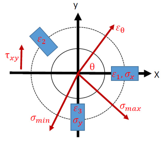
Figure 1.
Schematic highlighting a typical clockwise strain gauge with defined coordinate system.
In case of the incremental HDM, by incrementally removing the stressed material the surface deformations are measured at a sequence of steps using the strain gauges. From data obtained, the in-depth non-uniform profiles of residual stress are derived. For such purpose, Equation (1) can be developed with the incremental integral formalism.
The coefficients Cklij inside the matrix [C]ij are determined not only by the residual stress in the last increment, but also by the residual stresses of all previously drilled increments. Figure 2 schematically highlights the procedure of constituting the calibration coefficients matrix [C11]ij using the incremental HDM. Initially, the first layer is drilled and C1111 defines the influence of the stress σ1 (present in the 1st increment) on the strain ε1. Next, the second layer is drilled. C1121 and C1122, respectively, define the influences of the stress σ1 imposed in the 1st increment and the stress vector σ1 imposed in the 2nd increment on the strain ε1 measured. Following the same procedure for the subsequent steps, one can understand how C1131, C1132 and C1133 can be obtained.
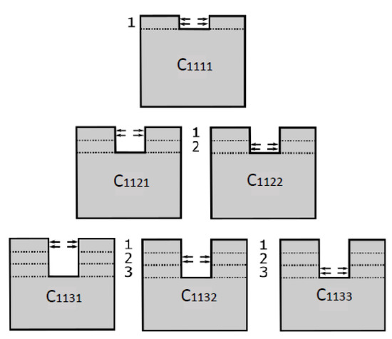
Figure 2.
Schematic detailing the stress state and hole depth considered to obtain the calibration coefficients for the initial three drilling steps.
Local heterogeneity and defects like voids and small cracks can be present in the sample, eventually leading to unequal strain values in the mirror position of the unidirectional FRP samples. In addition, if delamination occurs during the drilling process, additional anomalies can occur eventually affecting the accuracy of the experimentally determined results. The use of non-destructive characterization techniques such as computed tomography (CT) for detecting these defects during drilling is not possible in a robust way due to experimental restrictions. However, solely based on the analysis of data provided by the special strain gauge rosette depicted in Figure 3a critical evaluation of the results obtained is feasible. For achieving the aim of minimizing the errors caused by the aforementioned factors, a special strain gauge with eight grids is employed in the present work for acquiring sufficient strain information in all directions during drilling. This strain gauge will further be the key toward investigation of residual stresses in composites and hybrid materials with a more complex stacking sequence. For evaluating the residual stresses in the present work, only the strain information of three grids from the strain gauge is required due to the type of samples considered (c.f. Section 3). The position of the grids 1 to 8 is shown in Figure 3, and eight different combinations of strain gauge grids, (1, 2, 3), (2, 3, 4), (3, 4, 5), (4, 5, 6), (5, 6, 7), (6, 7, 8), (7, 8, 1), (8, 1, 2), are evaluated for determining residual stresses. An anomaly in the results due to local heterogeneity and defects can be immediately detected by using this special strain gauge. For measuring the residual stresses in FRP, the strain gauges 1 and 5 were always aligned with the fiber direction X. The impact of the misalignment of the strain gauge on the resulting residual stress was already discussed in [17].
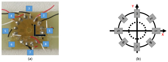
Figure 3.
(a) Sample and (b) sketch of the strain gauge rosette with eight grids used for measuring strains in glass fiber reinforced plastic (GFRP) upon drilling.
2.2. Calibration Coefficient Calculations
As the integral method is applied in the present work, the calibration coefficients for evaluating the residual stress from measured strains need to be calculated using FEA. The procedure for calculating the calibration coefficients is carried out using the software ABAQUS/Standard. To simulate the drilling process to obtain the calibration coefficients, a cylindrical model with orthotropic elastic material behavior was employed, where the ply orientation of the fiber in the FRP is defined in a local coordinate system. As shown in Figure 4, the model is comprised of the hole with a diameter of 2 mm and the outer part with a diameter of 50 mm. The whole model is meshed by about 200,000 eight-node solid elements of type C3D8R. Figure 4 shows the FEA model used including details such as the local mesh refinement in the direct vicinity of the drilled hole as well as the adopted local coordinates for imposing the load at the hole boundary. In the present work, the strains ε1 and ε5 are aligned with the fiber direction X of the composite.
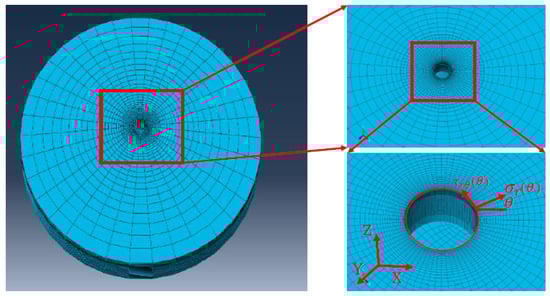
Figure 4.
Calculation of calibration coefficients using an ABAQUS finite element analysis (FEA) model: local mesh refinement in the direct vicinity of the drilled hole and imposed loads at the hole boundary.
Directly simulating the drilling process in a stressed sample to determine the calibration coefficients is complex. Alternatively, based on the principle of superposition, the strain relieve process by drilling can be simulated by prescribing loads opposed to the faces of the hole of an unstressed specimen, such that a complex simulation of the residual stress relieve process from the stressed model can be avoided. In the present study, the unit loads are applied in successive steps for each layer (c.f. Figure 2). To obtain the calibration coefficients [C]ij in Equation (2) in the orthotropic materials, three load cases are required to be applied for each drilling increment respectively, i.e., = 1, = 1 and = 1. To enable the application of a defined stress state equivalent to the released stresses within an increment during the drilling process, the in-plane stress components , and are converted to and in a radial coordinate system for prescribing the loads at the hole boundary (c.f. Figure 4).
Figure 5 shows the imposed mechanical boundary conditions for FRP/steel hybrid and FRP samples, where the circular boundaries of the bottom surface are completely fixed in all directions, while the part of the model below the hole is allowed to deform freely. Readers are referred to [8,14] for more information on calculation of the coefficients of orthotropic materials. The calibration coefficients rely on the type of the strain gauge and the material properties of the hybrid component considered. The hole geometry and the type of the strain gauge were considered to be always the same in the present study, thus, only the differences in material properties had to be considered. Based on these boundary conditions, the calibration coefficients for the four different types of samples investigated in the present work were calculated. In-depth discussion of the results obtained will be presented in the remainder of this paper.
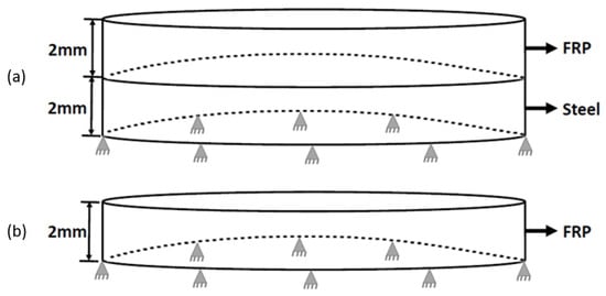
Figure 5.
Imposed mechanical boundary conditions for (a) FRP/steel hybrid and (b) FRP samples.
3. Experimental Procedure and Microstructure Characterization
3.1. Sample Preparation
In the present study, unidirectional GFRP (UD-GFRP) and unidirectional CFRP (UD-CFRP), as well as unsymmetric UD-GFRP/steel and UD-CFRP/steel hybrid composites were manufactured through the prepreg-press-technology always using the same process parameters; see [20] for more information on the manufacturing technology. UD-FRP/steel hybrid composites are characterized by outstanding specific stiffness and strength. When such structures are uniaxially loaded, generally only fibers are applied in the load direction. Therefore, metal layers are capable of substituting other ply orientations. By using such kind of hybridization, the stiffness and strength in the fiber direction of the hybrid sample are not reduced. However, the residual strength and energy absorption capacity for crashworthiness are improved in comparison with pure UD-FRP [3]. All FRPs used in present work are unidirectional. However, for better readability the terms ‘unidirectional’ and ‘UD’, respectively, will not always be provided.
The FRP/steel hybrid samples were manufactured by inserting the already processed steel sheet with a thickness of 2 mm into a heated die with dimensions of 100 mm × 250 mm × 20 mm. Then, the unidirectional glass/carbon fiber prepregs with the same thickness of 2 mm (9 plies) were pressed onto the metal sample using a heated punch. The types of glass/carbon fiber prepregs used were G U300-0/NF-E506/26% (with epoxy resin content of 26%) and C U255-0/NF-E322/37% (with epoxy resin content of 37%), respectively. The steel employed was HC340LA (microalloyed steel). Note that the steel sample before hybridization was not curved and heat treated, thus, it features initial residual stresses to a certain degree (the actual value was measured using the HDM and adequate strain gauges (Höttinger Baldwin Messtechnik GmbH, Darmstadt, Germany); see [17] for more details). Here, it is important to note that the initial residual stress values of different metal sheets used for hybridization could be slightly different. The epoxy resin acts as an adhesive to promote the fiber-matrix impregnation as well as to bond the metal and the GFRP/CFRP in the curing process of the GFRP/CFRP. Before manufacturing, the surface of the metal side was finished using a sandblasting process to increase the surface roughness of the metal (Ra = 35 μm), eventually improving the adhesion between the metal and the FRP. For manufacturing the symmetric GFRP and CFRP (c.f. Figure 6a,b), the unidirectional GFRP/CFRP prepregs were directly placed on the tool of the same machine and then pressed using the heated punch in the same fashion. All samples were processed using a pressure of 0.4 MPa and a temperature of 160 °C with a constant curing process time of 18 min. Afterwards, the samples which were not further pressed were cooled down in laboratory atmosphere with a cooling rate of approximately 100 °C/min.
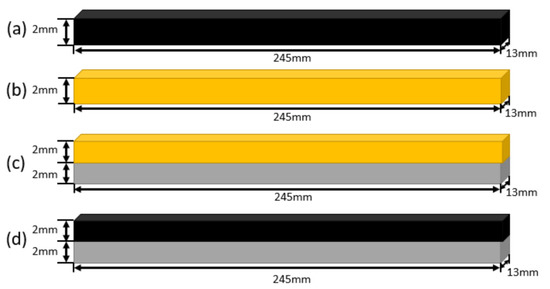
Figure 6.
Dimensions of (a) symmetric carbon fiber reinforced plastic (CFRP), (b) symmetric GFRP, (c) unsymmetric GFRP/steel and (d) unsymmetric CFRP/steel. The CFRP is colored black, the GFRP orange and the steel grey.
Figure 6 shows the dimensions of the samples, which were cut from the fully processed blanks with dimensions of 100 mm × 250 mm (the thickness of the samples is either 2 mm or 4 mm). Figure 7a,b show the final shape of the samples directly after they were removed from the tool and cut (using a conventional cutting machine with a cooling agent) from the completely processed plate in side and top views, respectively. The deformation of the samples as induced by the release of the residual stresses can be directly seen in the side view. The release of residual stress in the process of removing the samples from the tool is dominant and the magnitude of warpage depends on the material considered; see Section 4.3 for more details. Table 1 provides an overview of the experimentally determined mechanical properties of CFRP, GFRP and the steel used for realization of the hybrid composites in present work. Values obtained were determined according to DIN EN ISO 527, DIN EN ISO 14129 and DIN EN ISO 6892-1.
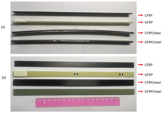
Figure 7.
Final shape of the fabricated samples after removal from the tool and subsequent cutting depicted in (a) side view and (b) top view (points marked A and B indicate the two positions considered for determination of residual stresses to be discussed in the remainder of present work).

Table 1.
Relevant mechanical properties of the respective parts of the hybrid samples.
3.2. Microstructure Characterization of the Samples
The bonding of dissimilar materials has proven to be challenging and eventually strongly affects the mechanical performance of the hybrid composite [21]. Figure 8 shows optical micrographs of the cross-sections highlighting the microstructure in the direct vicinity of the interface of the dissimilar materials in GFRP/steel and CFRP/steel samples, which were cut alongside and perpendicular to the fiber direction, respectively. For optical microscopy (OM) using a Keyence VHX 600 (Keyence Corporation, Osaka, Japan), the samples were cut and mechanically ground down to a grit size of 2 µm. Surface roughness is one important factor influencing the bonding conditions and the resulting mechanical properties of the bonded samples. In the present work, the surface of the metal sheet was processed using sand blasting to increase the surface roughness (Ra = 35 μm). By doing so, the epoxy resin in the curing process was able to flow into the grooves eventually increasing the contact area. Finally, the mechanical interlocking properties were improved. In addition, as shown in Figure 8, no obvious defects appear directly at the interface. Thus, it can be deduced that good bonding between the CFRP/GFRP and the steel prevails.
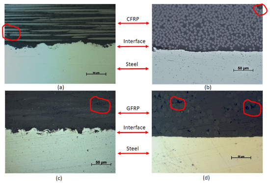
Figure 8.
Cross-sections highlighting the microstructures of (a) CFRP/steel sample cut along the fiber direction, (b) CFRP/steel sample cut perpendicular to the fiber direction, (c) GFRP/steel sample cut along the fiber direction and (d) GFRP/steel sample cut perpendicular to the fiber direction, in the direct vicinity of the interface of the dissimilar materials (dominant defects in the FRPs are highlighted with red circles).
The defects present, such as voids in the matrix, as shown in Figure 8, are induced due to many reasons, e.g., insufficient curing, trapped air and shrinkage of the resin, among others [21]. Clearly, these voids can have a significant effect on the final results, if they appear in high density and large size, respectively, in the area to be drilled beneath the attached strain gauge. A possible solution to this problem is to account for this effect in the FEA model to allow the corrected calibration coefficients to be calculated. In theory, the following procedure could be applied: characterization of the distribution and size of voids using computer tomography (CT) in a non-destructive manner followed by importing this information into the FEA model. However, conducting this procedure is very challenging such that further work is needed to address the prevailing issues listed in the following. Due to the requirement of obtaining information on all prevalent features including clusters of small voids (characteristic size of individual voids is highlighted in Figure 8), a small sample needs to be prepared for CT characterization in order to allow for sufficient resolution. Due to the optimized processing parameters employed, large voids have not been found in the samples characterized. Especially in case of the hybrid samples, the highly different contrasts stemming from the employed materials (imposed e.g., by their individual absorption characteristics) set further restrictions in terms of data analysis. Thus, in-depth analysis of full-scale samples used for HDM (c.f. Figure 7) currently is not robustly possible. So far, after microstructure characterization the strain gauge cannot be attached to the small samples (required for CT analysis) for residual stress measurement through HDM. Eventually, further work has to be conducted to optimize the procedure applied until now, however, this is clearly beyond the scope of the present work.
3.3. Experiment Details Related to Application of the Hole Drilling Method
In case of the hole drilling method, a small hole is incrementally drilled at the center of the strain gauge being attached on the surface of the sample. The released strain is recorded during drilling by the strain gauge. In the present work, to obtain sufficient information in all directions, a strain gauge with eight grids manufactured by Höttinger Baldwin Messtechnik (HBM) was used. A drilling tool made of tungsten carbide (ref H2.010, Komet) with a nominal diameter of 1 mm was employed. The hole was drilled incrementally with a step size of about 20 μm to ensure measurement accuracy. Moreover, an air turbine with a drilling speed of about 300,000 rpm (3 bar) was used combined with the orbital technique to drill the hole (diameter of 2 mm) to minimize the appearance of new stresses and delamination within the material [20]. The utilized drilling parameters are referred to as “optimal” ones. In the next section, the influence of drilling parameters on the residual stresses determined is highlighted.
3.4. Characterization of the Drilled Hole
To apply the HDM robustly, drilling of the hole needs to be carefully conducted to avoid introducing any misleading flaws and errors. In general, three main error sources have been reported in literature [12]: a non-cylindrical shape of the hole, introduction of additional stresses due to machining and eccentricity of the hole relative to the strain gauge rosette. Here, the influence of relevant drilling process parameters on the resulting residual stresses is investigated, and the quality of the drilled hole is evaluated by analyzing its geometrical characteristics.
After the drilling process, an optical microscope (Keyence VHX 600) was used to characterize the geometrical appearance of the hole to assess its quality. The drilled hole from the top view is shown in Figure 9, and it can be seen that the drilled hole has a round shape with a final diameter of around 2 mm. As mentioned in Section 3.3, a tool made of tungsten carbide (ref H2.010, Komet) with a nominal diameter of 1.0 mm was used for drilling. By using the orbital technique, the final hole diameter is around 2 mm, which is equal to the diameter value representative for the rosette. This ensures the reliability of the strain measurement. Furthermore, the concentricity of the rosette can be corroborated from the results presented.
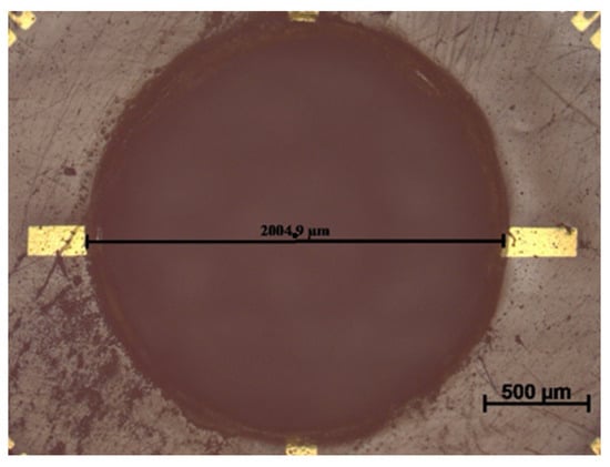
Figure 9.
Top view of the drilled hole in the GFRP sample.
As mentioned in ASTM–E837 [12], the drilling process can be conducted down to a depth characterized by a 0.4 multiple of the diameter of the hole for the case of non-uniform residual stresses. A hole with a diameter of around 2 mm was drilled, as shown in Figure 9. Thus, a maximum drilling depth of 800 μm was considered here. The cross-section of the drilled hole in the GFRP is shown in Figure 10. Despite the micrograph only providing a two-dimensional image of the hole, important information can be gained: (1) the final depth of the hole is very close to the targeted value, eventually demonstrating the good controllability of the drilling device (the depth was controlled using a micrometer gauge with a resolution of 2 μm); (2) the side face of the hole is vertical. In combination with the round shape of the hole seen in the top view (c.f. Figure 9), one can deduce that the drilled hole has an almost perfect cylindrical shape; (3) neither apparent damage around the hole nor cracking on the lateral face is found.
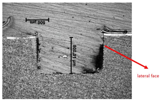
Figure 10.
Cross-sectional view of the drilled hole in the GFRP sample.
The used cutting tool (ref H2.010, Komet) is characterized by a chamfer in the corner of the edges. As detailed in [22], the use of the orbital drilling technique can avoid geometrical variations efficiently. However, the chamfers are still directly transferred to the hole bottom geometry, which can be seen in Figure 10. In the case of the model applied in FEA, a perfect cylindrical hole orthogonal to the surface with a flat bottom is assumed and established. Clearly, this effect may lead to errors, however, these are not considered in the present work. Furthermore, the results at a depth of 700 to 800 μm are excluded from analysis.
4. Results and Discussions
4.1. Calculated Calibration Coefficients
The way of calculating the calibration coefficients was already introduced in Section 2.2. This part lists the calculated calibration coefficients and further highlights the dependence of the coefficients on the mechanical properties of the samples. In the present study, a strain gauge with eight grids was applied as shown in Figure 3. It has to be emphasized that only three gauges are required for residual stress evaluation in the present work. Here, only the calibration coefficients for the grids No. 1 to 3 (c.f. Figure 3) are detailed. The angles of these grids with respect to the fiber direction are 0°, 45° and 90°, respectively. All further coefficients are provided in the supplementary material.
Table 2 lists the calculated calibration coefficients Cklij for GFRP for the first three increments, where each increment size is 20 μm. Figure 5 (detailed in Section 2.2) schematically highlights the boundary conditions for assessing the results given in Table 2. From Table 2 it can be seen that C31, C13 and C33, related to the first increment, are very small. Here, C31 is taken as one example for explaining the reasons. To obtain C31, a uniform load needs to be prescribed on the wall of the hole. Under such load, the strain obtained in grid 3 orthogonal to the fiber direction is small, thus yielding a small value for C31. Following the same argumentation, it becomes clear why the values of C13 and C33 are also small. For a given layer, the absolute values of the components in each matrix in Table 2 decrease from left to right. The reason for this trend is that the force imposed on the bottom layer (c.f. Figure 5) leads to smaller deformation on the surface of the sample than a force imposed in the upper layer. Based on this trend, it can already be concluded that a limit related to the maximum depth prevails for the HDM. Another trend is obvious: when the depth of the drilled hole increases, for each submatrix in Table 2 the absolute values are increased. Obviously, the stiffness of the material is reduced. As a consequence, the influence of the stress imposed on the first layer on the strain increases, eventually leading to larger calibration coefficients. The calibration coefficients were calculated by imposing stress boundary conditions in a radial coordinate system and they are a function of the material properties and the thickness of the sample, as well as the type and the position of the used strain gauge. In general, it can be concluded that the “+“ sign indicates the model is in tension while the “−“ sign implies it is in compression in the imposed force direction. In the incremental HDM, the calibration coefficients are determined not only by the imposed stresses in the last increment, but also by the values of all previously drilled increments. This implies that as more increment layers are drilled, the explanation of the results becomes more complex.
Table 2.
Calibration coefficients Ckl11*10−6 for the GFRP sample. Values are related to the first three increments in the framework of the integral method. See text for details.
The calculated calibration coefficients Ckl11 for different samples (c.f. Figure 6) related only to the first increment in the framework of the integral method are listed in Table 3. It can be seen that in all samples the values of C3111, C1311 and C3311 again are much smaller than the other components. Most importantly, the calibration coefficients are affected significantly when different material combinations are considered. C1111 is chosen as an example to illustrate the influence of the individual material properties on the residual stresses (the latter being detailed in the following sections). As shown in Table 3, the absolute value of C1111 for GFRP is much larger as compared to the respective value for CFRP. This observation can be explained as follows: C1111 can be obtained by imposing a uniform stress value σx. Loaded to the same stress level, the strain measured by grid 1 in the case of CFRP is smaller than in the case of GFRP, as the Young’s modulus of CFRP in the fiber direction is much higher than for GFRP. This leads to a calibration coefficient C1111 of CFRP being significantly smaller, as in the case of GFRP. As a second example, the results between CFRP and the CFRP/steel composite are compared. Imposed by hybridization, the Young’s modulus of the CFRP/steel composite is higher than in the case of pure CFRP, as implied by Table 1. This yields a coefficient C1111 of the hybrid/steel hybrid composite smaller than in the case of pure CFRP. The same relation can be deduced when comparing the coefficients C1111 of GFRP and the GFRP/steel hybrid composite. Other values listed in Table 3 can be explained in the same way. All calculated coefficients contribute to the explanation of the residual stresses finally determined.
Table 3.
Calibration coefficients Ckl11*10−6 for the four different samples considered. Values are related to the first increment in the framework of the integral method.
4.2. Strain Measurement
In the case of pure polymers, time-dependent effects imposed by loading of the tool while drilling have to be considered; see [16] for more information. The present part is to investigate whether these effects are also as influential in the case of the GFRP sample. Figure 11 shows the strain measurement in the case of the GFRP sample resolved for the first three drilling increments, where the strain information is recorded every 2 s by a strain measurement amplifier PICAS (PEEKEL Instruments Company, Bochum, Germany). Even if a strain gauge with eight grids is used, only the strain information from one grid is shown in Figure 11 to reveal the visco-effect. When the cutter is pushed and then rotated into the sample with a drilling speed of about 300,000 rpm, the rotation of the cutter produces high shear forces, eventually deforming the material in the vicinity of the hole. Thus, it can be seen that the strain is rapidly decreased to −80 μm. After the first drilling step, the cutter is completely removed from the sample. Then, the material is relaxed and the strain is increased to a positive value. Obviously, strain data already become stable after 30 s (after tool removal), which is much shorter than in the case of pure polymer materials (where time intervals around 6 min were reported [19]). This indicates that the visco-effect in the case of GFRP is not as strong as for pure polymer materials due to the glass fiber reinforcement. Certainly, it is not recommended to analyze the strain directly after drilling for calculation of residual stresses. To ensure a sufficient stability of data, a delay time after drilling is required for releasing the strain values of each drilling step. In the present work this is set to 90 s. In Figure 11, it can be further seen that the strain increases when a higher number of layers of the material is drilled. This observation holds true for CFRP as well.
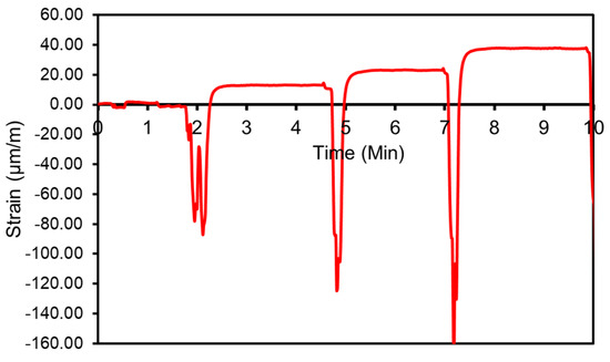
Figure 11.
Strain measurement in GFRP focusing on the first three drilling increments. Data were recorded every 2 s.
Figure 12 shows the relaxed elastic strains for GFRP taking into account the delay time of 90 s mentioned in the previous paragraph for each drilling increment. Strains are determined using the special strain gauge with eight grids (c.f. Figure 3). In all measurements, the strain gauges 1 and 5 are aligned in the fiber direction, and the strain gauges 3 and 7 are aligned transverse to the fiber direction. It is seen that the strains in the directions of 1 and 5 are positive and very close, while the strains in other directions are negative. The magnitude of strains in all directions increases as the drilling depth increases. The strains recorded in mirror positions of the strain gauge are very close, except those of directions 3 and 7, which can be explained by local heterogeneity (such as depicted in Figure 8).
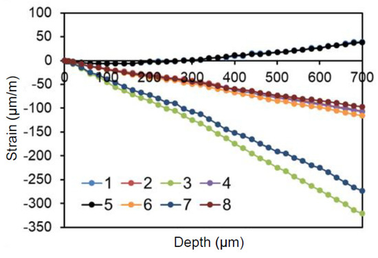
Figure 12.
Determination of strains for GFRP using the customized eight grid strain gauge.
4.3. Experimentally Determined Warpage
During manufacturing of the different types of samples, residual stresses are induced to varying degrees due to several reasons, eventually leading to warpage. Figure 13 shows a schematic highlighting the warpage values obtained for the fabricated samples of GFPR, CFRP, GFRP/steel and CFRP/steel (c.f. Figure 7a) after they were removed from the tool and cut to meet the final sample dimensions (c.f. Section 3). Sample handling and cutting is assumed not to substantially affect residual stresses being present at this point as the dimensions of samples used for further characterization in the fiber direction are still relatively large. From Figure 13, it is clearly seen that the warpage of the unsymmetrical FRP/steel hybrid samples is significant, while the warpage of the symmetrical unidirectional FRP samples is very small (around 0.3 mm) and, thus, is neglected here. The warpage was measured using three-dimensional digital image correlation (DIC).
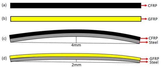
Figure 13.
Schematic highlighting relevant values related to warpage of the fabricated samples after removal from the tool (a) CFRP, (b) GFRP, (c) CFRP/steel and (d) GFRP/steel.
Theoretically, the symmetric composite, e.g., the unidirectional FRP (after the sample is removed from the tool), does not deform as it satisfies the self-equilibrium conditions through the thickness of the laminate. However, in reality, the tool material usually has a higher thermal expansion coefficient than the FRP composite. In the curing process, the tool and the composite sample are pressed together under a certain pressure and temperature. This results in a shear interaction between the tool and the composite. When the composite is removed from the tool, the induced stress gradient is locked, causing the appearance of the warpage of the composite. The aforementioned reasons can explain why a small amount of warpage could be present in the relatively thin symmetric FRP composites after removal from the tool. In the present work, only minor warpage with values of around 0.3 mm is determined in the CFRP and GFRP samples.
The experimentally determined absolute value of warpage in the case of the unsymmetric CFRP/steel composite is around 4 mm, which is much higher than in the case of the GFRP/steel composite being characterized by a value of around 2 mm. This observation can be mainly explained by the fact that the difference of the coefficient of thermal expansion (CTE) between CFRP and steel is much higher than the difference between GFRP and steel; see Table 4 for the relevant thermal expansion coefficients. To substantiate the relevant mechanisms, a short description of the manufacturing/curing process of the hybrid laminates is given here. Firstly, the hybrid composite is heated to the curing temperature; the thin metal layer with a high CTE expands and then stretches the composite prepreg plies, which are characterized by a low CTE. Secondly, the sample is cured at a constant cure temperature for a certain time. In this process, a stable bond between the dissimilar materials is established. Finally, the sample is cooled down. With respect to the FRP/metal hybrid composite, the major share of residual stresses is formed in the cooling process. Eventually, the difference in CTE values between dissimilar materials is one of the key factors with respect to tailoring residual stresses, as has already been stated in [4,6,8].
Table 4.
Coefficient of thermal expansion (CTE) of CFRP, GFRP and steel forming the individual layers of the hybrid composite.
4.4. Residual Stresses Determined for GFRP
Figure 14a shows the experimentally determined residual stresses σx based on the eight chosen different combinations (c.f. Section 2.1) at the center (A point) in the GFRP component, as defined in Figure 7b. In Figure 14a, it can be seen that except the combinations of 2 and 6, the residual stresses σx of all other combinations show similar results. This result is thought to be related to the lack of strain information in the fiber direction in the case of the combinations 2 and 6 (i.e., none of the strain gauges is oriented parallel to the fibers). Tensile stresses with a value around 17 MPa close to the surface were measured, and it is seen that the magnitude of the stress values is reduced as the depth increases. At the depth of 0.1 mm, the residual stresses convert from tensile to compressive and then convert back to tensile stresses at the depth of 0.35 mm. Residual stresses are referred to self-balanced stresses remaining in the sample in the absence of external mechanical loads. As any composite is a complex material, the balance system becomes also complex. Thus, a tensile-compressive-tensile stress profile is observed. The absolute value of the maximum compressive stress is around 2.5 MPa at the depth of 0.18 mm. From a surface distance of 0.65 mm, a strong divergence of the residual stresses appears, which can be explained by the fact that as the depth increases, the surface strain response becomes insensitive to the effects of in-depth residual stresses. Figure 14b shows the experimentally determined residual stress results for σy at the center (A point) in the GFRP sample, as defined in Figure 7b, where again the eight different combinations of strain gauge grids are accounted for. In Figure 14b, it can be seen that close to the surface, σy tensile stresses with a maximum value of about 18 MPa prevail and then are reduced as the depth increases. At the depth of 0.12 mm, residual stresses convert to compressive residual stresses and then increase to the maximum compressive residual stress with the absolute value of 3 MPa at the depth of 0.2 mm.
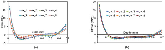
Figure 14.
Residual stress values determined by the hole drilling method (HDM) at center point A (shown in Figure 7b) with respect to (a) σx and (b) σy.
As discussed in ASTM E837-13a [12], many drilling process parameters can affect the accuracy of the residual stresses determined. In the present work, focus is on some key drilling process parameters, e.g., the drilling speed, the drilling increment size and the zero-depth choice. The determination of the zero-depth, which is defined as the surface of the sample, is very important for providing reliable results with respect to residual stresses. In the present work, the ideal zero-depth setting was carefully determined by removing the coating, the foil of the strain gauge and then the adhesives by successively drilling in steps of about 5 to 10 μm. After each drilling, the actual surface was carefully checked, and it was evaluated, using a camera, whether the cutter had already come into contact with the surface of the sample. As the color of the strain gauge rosette foil is very close to the GFRP sample, this imposed further difficulty in determining the real surface of the sample. Figure 15 shows the process of removing the strain gauge rosette foil step by step, including the initial stage, i.e., the cutter not yet drilled into the strain gauge (Figure 15a), some foil layers of the strain gauge being removed (Figure 15b) and the first view of the surface of the sample (Figure 15c).
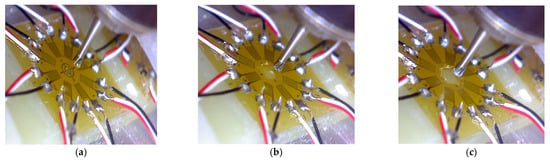
Figure 15.
Removal of the stain gauge rosette foil for precisely determining the surface of the sample via stepwise drilling. The following steps are highlighted: (a) before drilling, (b) intermediate stage (very thin foil film remained) and (c) the first view of the surface of the sample.
To achieve the aim of studying the effect of the choice of a non-exact depth setting on the resulting residual stresses, a series of non-adequate depth settings having different deviations from the ideal depth position were considered to evaluate the residual stresses; see Figure 16 for the results. Note that the label (0 μm) indicates the optimal zero-depth setting, while the other labels (30 μm and 60 μm) imply that the adopted zero-depth settings are 30 and 60 μm beneath the surface of the sample, respectively. Based on the results shown in Figure 16, it can be clearly seen that the consequences of an incorrectly assumed hole depth are most pronounced in the direct vicinity of the surface. When the hole depth increases, an overestimation of the correct residual stress values appears and then this effect diminishes. Furthermore, as the depth increases, the surface strain response becomes insensitive to the drilling process, thus leading to pronounced scattering of the residual stress results.
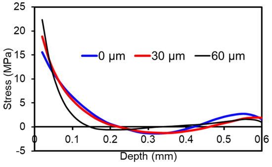
Figure 16.
The effect of zero-depth setting on the residual stress.
Undoubtedly, the drilling speed is one of the most important parameters that can influence the residual stress values determined. Two very adjacent points (assumed to be characterized by the same magnitude of prevailing residual stress states, however, not affecting each other) were drilled with the distance of 5 mm in one GFRP sample at fast and slow drilling speed. Here, fast drilling is characterized by a high drilling speed of 300,000 rpm, whereas slow drilling is linked to a drilling speed of 10,000 rpm. Figure 17 shows the resulting residual stresses as a function of the two different drilling speeds. It can be seen that the resulting residual stresses close to the sample surface obtained using fast drilling are smaller than in the case of slow drilling. This observation can be rationalized by the presence of machining-induced stresses (promoted by slow drilling) and, eventually, the fact that the released strain upon fast drilling is smaller than upon slow drilling due to the induced local plastic deformation in the latter case.
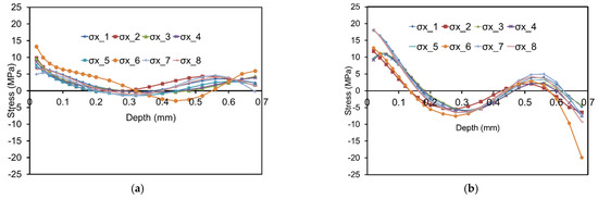
Figure 17.
Effect of drilling speed on the resulting residual stresses considering (a) fast and (b) slow drilling. For better resolution of results scales are different.
By using the incremental HDM, the in-depth residual stress profile can be determined. For each drilling increment the stress is assumed to be homogeneous. This assumption stands as long as the thickness of each layer is small enough. However, the thickness cannot be infinitely small. If the thickness is very small, not only the processing time is significantly increased, but also more contact between the tool and the material can be prejudicial, eventually leading to measurement errors. Figure 18 shows the residual stresses experimentally determined applying a large increment size of 80 μm. It is seen that the residual stresses obtained are characterized by pronounced scatter in the case of all combinations (c.f. Figure 3), indicating the presence of larger errors. Based on the analysis in this part, optimal drilling parameters could be deduced. These were applied and are further evaluated in the remainder of the present work.
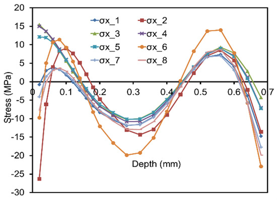
Figure 18.
Resulting residual stresses with a large increment size of 80 μm.
4.5. Reliability of the Residual Stress Measurement in Case of GFRP
The reliability of residual stress measurements through the HDM using optimal drilling process parameters detailed in Section 3.3 and Section 3.4 needs to be validated. In the present work, a mechanical bending experiment is used to test the measurement reliability with respect to prevailing stresses in GFRP with the dimension given in Figure 6b. The experimental setup is shown in Figure 19. The validation process is comprised of three main steps. In the first step, without prescribing any extra loading, the residual stress on a single point at a distance of 40 mm from the edge of the sample is measured through HDM, see Figure 20a for the results. The bending stiffness of the GFRP is not very high. In order to avoid bending of the sample during drilling, a vernier height gauge is placed beneath the GFRP sample with an initial gap of 1 mm (c.f. Figure 19). At the second step, one side of the same GFRP sample is clamped and the other side is loaded with a weight of 467 g as shown in Figure 19. By using elastic FEA, the stress distribution in the whole sample can be calculated. Finally, upon loading, one hole adjacent to the previous one is drilled with a superimposed external load for stress analysis; see the result in Figure 20b. The results obtained are expected to be the sum of the stresses induced by loading and the initially determined process-induced residual stresses. This assumption holds true as long as without external loading the process-induced residual stresses of two adjacent points are very similar. Based on FEA, external loading with a weight of 467 g at one side of the sample induces surface stress of about 70 MPa at the drilling point. Direct comparison of the difference between initial residual stress and the total stresses upon loading (with the values calculated using FEA) is a reliable way to check the reliability of the measurement. Figure 20c shows the comparison of results, where the black dashed line corresponds to the calculated value induced by bending (simple elastic FEA model). A good agreement between the residual stress difference and the numerical values is obtained, implying the reliability of the measurement. The minor differences seen can be explained by the following reasons: (1) the appearance of plastic deformation, which was not considered in numerical simulation and (2) the initial process-induced residual stresses in adjacent points are not exactly equal.
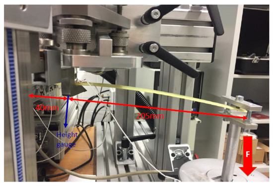
Figure 19.
Experimental set-up used for evaluating the reliability of the residual stress measurements conducted.
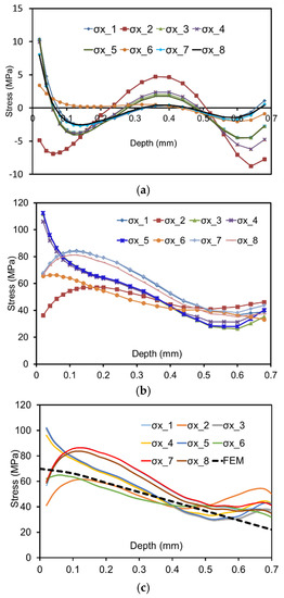
Figure 20.
(a) Residual stress σx in a GFRP sample without superimposed external loading, (b) measured residual stress σx with loading and (c) validation of the obtained values. See text for details.
4.6. Residual Stresses Comparison of GFRP, CFRP, GFRP/Steel and CFRP/Steel Composites
The objective of this part is to compare the residual stresses of GFRP, CFRP, GFRP/steel and CFRP/steel hybrid composites, which all were manufactured employing the same process parameters. The residual stresses of the samples were measured after they were removed from the tool and cut from the completely processed blank.
Figure 21 shows residual stresses σx obtained for GFRP, CFRP, GFRP/steel and CFRP/steel composites, respectively, where all samples were measured at center point A (c.f. Figure 7b). For clarity, only σx calculated based on data from the first configuration (1, 2, 3) (c.f. Figure 3) is plotted in Figure 21. The residual stress profiles of all samples generally are characterized by a similar trend. Close to the surface, residual stresses are characterized by the highest absolute values and tensile stresses, respectively. Afterwards, stresses decrease as the depth increases. CFRP and GFRP are quasi-symmetric composites, thus, only minor residual stresses were released during the removal process from the die, as already deduced from minimum values found for warpage (c.f. Figure 7).
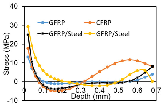
Figure 21.
Residual stresses σx experimentally determined by the HDM for GFRP, CFRP, GFRP/steel and CFRP/steel composites. See text for details.
On the contrary, for unsymmetric FRP/steel composites residual stresses were released to a significant amount, implied by the warpage of up to 4 mm (c.f. Figure 13). The larger the warpage is for a given material, the higher the residual stresses being already released. Obviously, stiffness of the sample has to be taken into account at this point. Release of residual stresses has to be in line with predictions of bending theory. Based on all results obtained (c.f. Figure 21), important conclusions can be drawn: (1) residual stresses in CFRP are higher than in GFRP, as Young’s modulus of CFRP is higher than for GFRP and the difference in CTE between carbon fiber and matrix is more pronounced; (2) the process-induced residual stresses in the CFRP/steel hybrid sample are higher than in the GFRP/steel sample, and certainly also higher than in pure FRP. This again can be explained by the difference in CTE between dissimilar materials; (3) no presence of warpage after the sample is removed from the tool only implies that the sample satisfies the self-balancing conditions, rather than indicating that the sample is in stress-free state. The remaining residual stress in the sample should be considered in any case.
5. Conclusions
In the present work, residual stresses and warpage of glass/carbon fiber reinforced plastic (GFRP/CFRP) and hybrid components directly realized by the manufacturing process were experimentally determined. All samples were fabricated through the prepreg-press-technology using the same process parameters. The residual stresses of these components were experimentally determined through the hole drilling method (HDM), employing a formalism allowing the residual stresses for orthotropic materials to be evaluated by calculating the calibration coefficients using finite element analysis (FEA) considering real material configuration and mechanical properties of the samples. The warpage induced by residual stresses was measured after the samples were removed from the tool and cut to the final shape. The effects of drilling process parameters of HDM, e.g., the drilling speed, the drilling increment and the zero-depth setting, on the resulting residual stresses of GFRP were investigated. The residual stresses and warpage determined for four different types of samples were compared and were analyzed in depth. The following conclusions can be drawn:
- In the case of the HDM, the zero-depth needs to be carefully determined. A non-exact zero-depth setting strongly biases the resulting residual stresses.
- With a large drilling increment size, the residual stress results suffer from pronounced scatter. It was also found that the resulting residual stresses close to the surface obtained after fast drilling are smaller than after slow drilling. This fact is attributed to the presence of machining induced stresses and local plastic deformation.
- Based on results presented and discussed, optimal drilling parameters were concluded. The reliability of the determination of residual stresses in GFRP using the optimal drilling parameters could be positively validated using mechanical bending tests.
- Obvious warpage induced by residual stresses was observed in the unsymmetrical composites. Only minor warpage was found in symmetrical FRP, the latter most probably being induced by shear forces between the FRP and the tool. The warpage of the CFRP/steel hybrid composite is larger than for the GFRP/steel hybrid composite, due to a higher difference in CTE between CFRP and steel.
The results obtained in the present work can be extended to other hybrid materials and used for designing multi-stable laminates for application in adaptive structures. In future work, extending the presented work to symmetrical and unsymmetrical hybrid composites with more complex lay-up configurations is intended. Furthermore, analysis of residual stress distributions in the direct vicinity of the boundary layer is of the highest importance for in-depth evaluation of contributing factors on the overall residual stress state. This will be accomplished by direct comparison of results being measured using the HDM and high-energy X-ray diffraction.
Author Contributions
Conceptualization, T.N. and T.T.; methodology, T.W.; software, T.W.; validation, T.W., W.Z. and S.T.; formal analysis, T.W.; investigation, T.W.; writing—original draft preparation, T.W.; writing—review and editing, T.W., W.Z., S.T., T.N. and T.T.; supervision, T.N. and T.T.; project administration, T.W., W.Z. and S.T.; funding acquisition, T.N. and T.T. All authors have read and agreed to the published version of the manuscript.
Funding
This research was funded by the Deutsche Forschungsgemeinschaft (DFG) with the project number of 399304816.
Institutional Review Board Statement
Not applicable.
Informed Consent Statement
Not applicable.
Data Availability Statement
Data available upon reasonable request.
Conflicts of Interest
The authors declare no conflict of interest.
References
- Saleh, M.N.; El-Dessouky, H.M.; Saeedifar, M.; De Freitas, S.T.; Scaife, R.J.; Zarouchas, D. Compression after multiple low velocity impacts of NCF, 2D and 3D woven composites. Compos. Part A Appl. Sci. Manuf. 2019, 125, 105576. [Google Scholar] [CrossRef]
- Saeedifar, M.; Saleh, M.N.; El-Dessouky, H.M.; De Freitas, S.T.; Zarouchas, D. Damage assessment of NCF, 2D and 3D woven composites under compression after multiple-impact using acoustic emission. Compos. Part A Appl. Sci. Manuf. 2020, 132, 105833. [Google Scholar] [CrossRef]
- Reuter, C.; Tröster, T. Crashworthiness and numerical simulation of hybrid aluminium-CFRP tubes under axial impact. Thin-Walled Struct. 2017, 117, 1–9. [Google Scholar] [CrossRef]
- Tinkloh, S.; Wu, T.; Tröster, T.; Niendorf, T. A micromechanical-based finite element simulation of process-induced residual stresses in metal-CFRP-hybrid structures. Compos. Struct. 2020, 238, 111926. [Google Scholar] [CrossRef]
- Hufenbach, W.; Gude, M.; Kroll, L. Design of multistable composites for application inadaptive structures. Compos. Sci. Technol. 2002, 16, 2201–2207. [Google Scholar] [CrossRef]
- Daynes, S.; Weaver, P. Analysis of unsymmetric CFRP–metal hybrid laminates for use in adaptive structures. Compos. Part A Appl. Sci. Manuf. 2010, 41, 1712–1718. [Google Scholar] [CrossRef]
- White, S.R.; Hahn, H.T. Cure cycle optimisation for the reduction of processing-induced residual stresses in composite materials. J. Compos. Mater. 1993, 27, 1352–1378. [Google Scholar] [CrossRef]
- Prussak, R.; Stefaniak, D.; Hühne, C.; Sinapius, M. Evaluation of residual stress development in FRP-metal hybrids using fiber Bragg grating sensors. Prod. Eng. 2018, 12, 259–267. [Google Scholar] [CrossRef]
- Rossini, N.; Dassisti, M.; Benyounis, K.; Olabi, A.-G. Methods of measuring residual stresses in components. Mater. Des. 2012, 35, 572–588. [Google Scholar] [CrossRef]
- Huang, X.; Liu, Z.; Xie, H. Recent progress in residual stress measurement techniques. Acta Mech. Solida Sin. 2013, 26, 570–583. [Google Scholar] [CrossRef]
- Magnier, A.; Zinn, W.; Niendorf, T.; Scholtes, B. Residual Stress Analysis on Thin Metal Sheets Using the Incremental Hole Drilling Method—Fundamentals and Validation. Exp. Tech. 2019, 43, 65–79. [Google Scholar] [CrossRef]
- ASTM International. Standard Test Method for Determining Residual Stresses by the Hole-Drilling Strain-Gage Method; ASTM E837-13; ASTM International: West Conshohocken, PA, USA, 2013. [Google Scholar]
- Gong, X.-L.; Wen, Z.; Su, Y. Experimental determination of residual stresses in composite laminates [02/θ2]s. Adv. Compos. Mater. 2014, 24, 33–47. [Google Scholar] [CrossRef]
- Schajer, G.S.; Yang, L. Residual-stress measurement in orthotropic materials using the hole-drilling method. Exp. Mech. 1994, 34, 324–333. [Google Scholar] [CrossRef]
- Akbari, S.; Taheri-Behrooz, F.; Shokrieh, M. Characterization of residual stresses in a thin-walled filament wound carbon/epoxy ring using incremental hole drilling method. Compos. Sci. Technol. 2014, 94, 8–15. [Google Scholar] [CrossRef]
- Magnier, A.; Scholtes, B.; Niendorf, T. On the reliability of residual stress measurements in polycarbonate samples by the hole drilling method. Polym. Test. 2018, 71, 329–334. [Google Scholar] [CrossRef]
- Wu, T.; Tinkloh, S.R.; Tröster, T.; Zinn, W.; Niendorf, T. Determination and Validation of Residual Stresses in CFRP/Metal Hybrid Components Using the Incremental Hole Drilling Method. J. Compos. Sci. 2020, 4, 143. [Google Scholar] [CrossRef]
- Magnier, A.; Wu, T.; Tinkloh, S.R.; Tröster, T.; Scholtes, B.; Niendorf, T. On the reliability of residual stress measurements in unidirectional carbon fibre reinforced epoxy composites. submitted.
- Magnier, A. Residual Stress Analysis in Polymer Materials Using the Hole Drilling Method-Basic Principles and Applications. Ph.D. Thesis, University of Kassel, Kassel, Germany, 2018. [Google Scholar]
- Lauter, C.; Reuter, C.; Wu, S.; Tröster, T. Large-Scale Production of High-Performance Fiber-Metal-Laminates by Prepreg-Press-Technology. Int. J. Mater. Metall. Eng. 2016, 10, 964–969. [Google Scholar]
- Mehdikhani, M.; Gorbatikh, L.; Verpoest, I.; Lomov, S.V. Voids in fiber-reinforced polymer composites: A review on their formation, characteristics, and effects on mechanical performance. J. Compos. Mater. 2019, 53, 1579–1669. [Google Scholar] [CrossRef]
- Nau, A.; Scholtes, B. Evaluation of the High-Speed Drilling Technique for the Incremental Hole-Drilling Method. Exp. Mech. 2012, 53, 531–542. [Google Scholar] [CrossRef]
- Vaggar, G.B.; Kamate, S.C.; Badyankal, P.V. Thermal Properties Characterization of Glass Fiber Hybrid Polymer Composite Materials. Int. J. Eng. Technol. 2018, 7, 455–458. [Google Scholar] [CrossRef]
- Ran, Z.; Yan, Y.; Li, J.; Qi, Z.; Yang, L. Determination of thermal expansion coefficients for unidirectional fiber-reinforced composites. Chin. J. Aeronaut. 2014, 27, 1180–1187. [Google Scholar] [CrossRef]
- Xu, G.; Deng, P.; Wang, G.X.; Cao, L.F.; Liu, F. Measurement of expansion coefficients of four steel types. Ironmak. Steelmak. 2013, 40, 613–618. [Google Scholar] [CrossRef]


Publisher’s Note: MDPI stays neutral with regard to jurisdictional claims in published maps and institutional affiliations. |
© 2021 by the authors. Licensee MDPI, Basel, Switzerland. This article is an open access article distributed under the terms and conditions of the Creative Commons Attribution (CC BY) license (http://creativecommons.org/licenses/by/4.0/).