Article

Identification of a Spatio-Temporal Temperature Model for Laser Metal Deposition

Department of Measurement and Control, Institute of System Analytics and Control, University of Kassel, 34125 Kassel, Germany
*
Author to whom correspondence should be addressed.
Metals 2021, 11(12), 2050; https://doi.org/10.3390/met11122050
Submission received: 11 November 2021 / Revised: 10 December 2021 / Accepted: 11 December 2021 / Published: 18 December 2021
(This article belongs to the Special Issue Additive Manufacturing Processes in Metals)

Abstract

:
Laser-based additive manufacturing enables the production of complex geometries via layer-wise cladding. Laser metal deposition (LMD) uses a scanning laser source to fuse in situ deposited metal powder layer by layer. However, due to the excessive number of influential factors in the physical transformation of the metal powder and the highly dynamic temperature fields caused by the melt pool dynamics and phase transitions, the quality and repeatability of parts built by this process is still challenging. In order to analyze and/or predict the spatially varying and time dependent thermal behavior in LMD, extensive work has been done to develop predictive models usually by using finite element method (FEM). From a control-oriented perspective, simulations based on these models are computationally too expensive and are thus not suitable for real-time control applications. In this contribution, a spatio-temporal input–output model based on the heat equation is proposed. In contrast to other works, the parameters of the model are directly estimated from measurements of the LMD process acquired with an infrared (IR) camera during processing specimens using AISI 316 L stainless steel. In order to deal with noisy data, system identification techniques are used taking different disturbing noise into account. By doing so, spatio-temporal models are developed, enabling the prediction of the thermal behavior by means of the radiance measured by the IR camera in the range of the considered processing parameters. Furthermore, in the considered modeling framework, the computational effort for thermal prediction is reduced compared to FEM, thus enabling the use in real-time control applications.

1. Introduction

Additive manufacturing (AM) enables the production of complex and customized parts using a focused heat source to fuse material in a layer-wise fashion. Depending on size, material, and complexity of the parts to be manufactured, different processes are used. In AM of metallic materials, laser metal deposition (LMD) can be used where the layer-by-layer part manufacturing is accomplished by an in situ delivery of powder material by a nozzle subsequently melted by the laser. Thereby, the resultant part quality in terms of its shape, micro-structure distribution, hardness, etc., is determined by many interconnected physical phenomena affiliated with the combination of the chosen process parameters [1]. The phase transition of the metallic material is a complex process depending on the spatial heat supply and dissipation. Moreover, the resultant spatially resolved thermal history of the part mainly effects its micro-structural distribution and thus is desirable to be predictable for optimization and control of the LMD process [2,3].
Due to the complexity of physical phenomena and the large amount of process variables involved, finite element methods (FEM) and computational fluid dynamics (CFD) are commonly used for modeling the LMD process [1]. While these models are suitable for process analysis if appropriated parametrized, they are generally too complex for control applications.
Commonly, works dealing with controller synthesis for laser-based AM processes assume solely temporal dynamics and, thus, use lumped parameter models (see, e.g., [4,5,6,7,8,9]). These lumped models neglect the spatial behavior of the thermal field or use an online adaption scheme together with an appropriate monitoring system to take the changing thermal dynamics in the AM process into account. For instance, Salehi and Brandt [4] measured the melt pool temperature using a two-color pyrometer and related it to the laser power by the use of a simple transfer function model to synthesize a PID controller. Song et al. [8,9] developed a state-space model for this purpose. Tang and Landers [5,6,7] proposed a transfer-function based model for the use in an online melt pool temperature controller where they take the time-varying temperature dynamics into account by using a Kalman-filter based adaption scheme.
The negligence of the spatio-temporal dynamics in modeling and control of the LMD process can cause geometrical instability or unwanted microstructural properties of the resultant part [10]. Therefore, more recently, Sammons et al. [11] proposed a multi-dimensional model of the layer deposition height used in a repetitive layer-to-layer control scheme. In order to parametrize the model, a system identification framework together with carefully conducted experiments is used. Cao and Ayalew [12,13,14] developed a Multi Input Multi Output (MIMO) surrogate model, considering the spatio-temporal dynamics relating the laser power and scanning speed to the deposition height and molten pool temperature. The surrogate model is a reduced lumped model description, and its parameters are identified using data obtained from FEM simulations of a multi-physics spatio-temporal model.
In this contribution, the thermal characteristics of the LMD process are modeled using a spatio-temporal input–output modeling approach relating the laser power to the measurement signal of an IR camera. Using an IR camera enables the spatially distributed measurement of the surface temperature and thus the monitoring of the thermal evolution of the produced part which mainly affects its micro-structure properties [1]. The original contribution of this work is the combination of spatio-temporal thermal measurements with a spatio-temporal modeling approach, i.e., the estimation of the model parameters of a partial recurrence equation model using the measurements of an IR camera. By doing so, a spatio-temporal temperature model of the LMD process is obtained. Based on this kind of model, distributed control strategies could be developed that may provide for a more accurate deposition process.
The remainder of the paper is organized as follows: the experimental setup together with operational conditions for data acquisition and the entire data pre-processing scheme are described in Section 2. In Section 3, the fundamentals of the spatio-temporal system identification are summarized. Furthermore, the used model is proposed together with the applied identification approaches. Modeling results considering real data of an LMD process are presented and discussed in Section 4.

2. Experimental Setup and Data
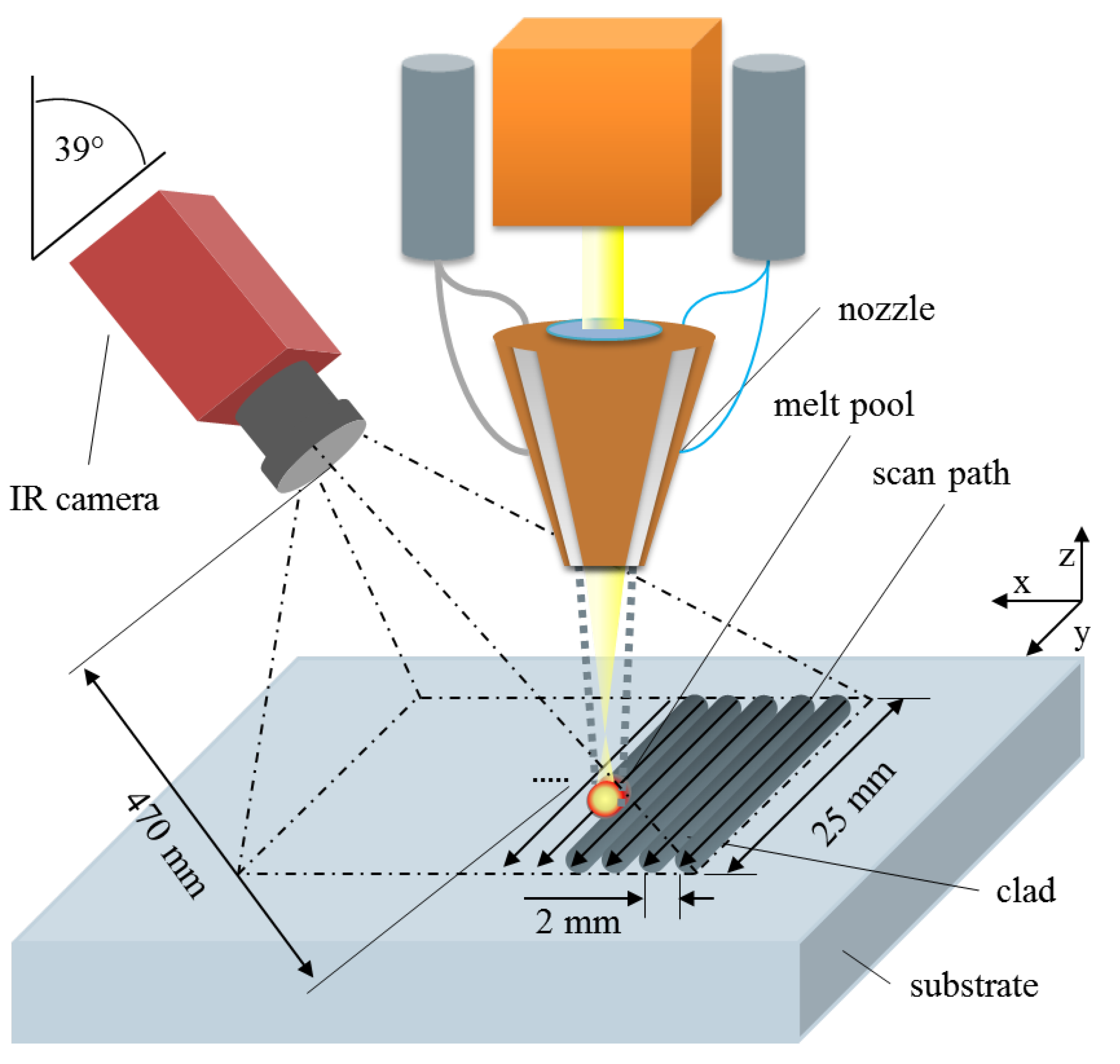
In this section, the data acquisition as well as the data pre-processing are discussed. The experimental setup is illustrated in Figure 1. The setup consists of two main components, the LMD unit and the measurement system based on an infrared camera, which are described in Section 2.1. This is followed by the experimental setup (see Section 2.2) and the used data preprocessing algorithms (see Section 2.3).

2.1. Hardware

2.1.1. Laser Metal Deposition System

The experiments were conducted using a laser processing setup consisting of a 2 k W multi-mode fiber-laser with a wavelength of 1070 n m (YLS-2000-S2, IPG Photonics, Burbach, Germany). The laser optics (MWO44, Kuka Industries GmbH & Co. KG, Würselen, Germany) were mounted to a six-axis robot (RV30-25, Kuka Industries GmbH & Co. KG, Obernburg, Germany). The experiments were performed with AISI 316 L powder with a grain size in the range of 50 μ m to 105 μ m . The shape of the particles was spherical. The powder was fed to a three-jet-nozzle (Fraunhofer ILT, Aachen, Germany) by a two-channel powder feeder (PF2/2, GTV Verschleißschutz GmbH, Luckenbach, Germany) using Argon carrier gas. A substrate of S235 steel was aligned to a baseplate before initiating deposition of the material. In order to prevent oxidation during fabrication, Argon shielding gas was used. The focal spot was positioned 85 m m from the workpiece, which resulted in a defocused laser spot size of approximately 2 m m at the substrate surface.

2.1.2. Measurement Equipment

For measurement of the thermal history, a cooled InSb mid-wave infrared (MWIR, λ cam = 2.0 μ m to 5.7 μ m ) camera (ImageIR 8380 hp, InfraTec GmbH, Dresden, Germany) was used. The camera has an array of 640 × 512 detector elements and has been radiometrically calibrated in sub-ranges by the manufacturer for a temperature range from 0 C to 2000 C (black body temperature, ε = 1 ). In order to be able to use several of the sub-ranges simultaneously, a multi-integration time mode or a rotating filter wheel can be applied. The rotating filter wheel was used for the performed measurements, so that a temperature range of 300 C to 2000 C ( ε = 1 ) is selected at an image frame rate of approx. 300 Hz . Due to the used macro lens, the geometric resolution of a single image point is approximately 70 μ m (IFOV) at the measurement distance of 47 c m with a zenith angle of 39 . The angular range is limited due to the laser optics and the protective frame of the build chamber. Within the selected arrangement of the experimental setup, the whole specimen is in the field of view of the camera. To protect the camera (see Figure 2) from the harsh process conditions, two protective arrangements were taken:
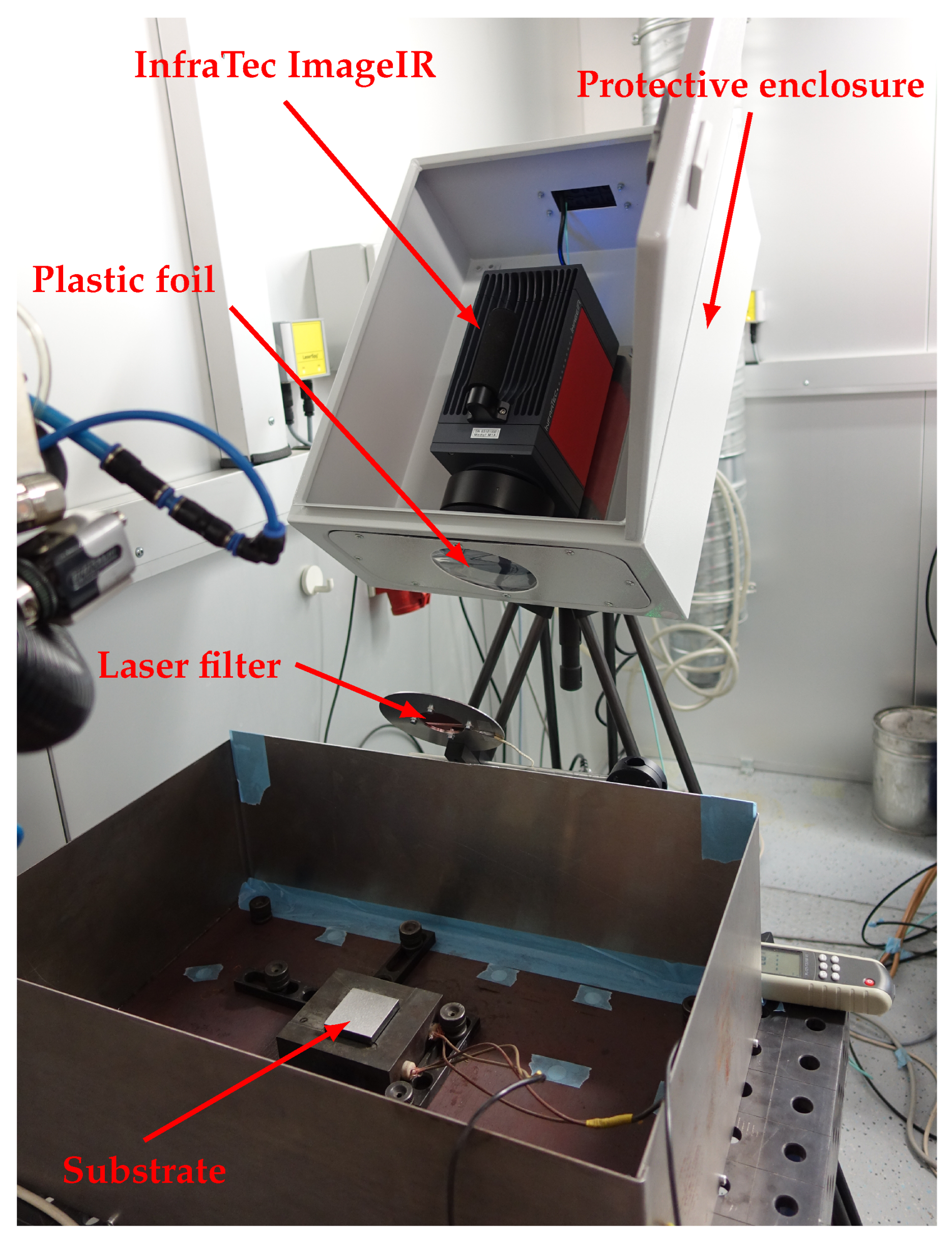
  • The camera is enclosed in a housing to prevent the metal powder dusts from entering into the camera. A hole was drilled into the housing’s metal plate at the camera’s field of view and a semi-transparent plastic foil was adhered to it.
  • The infrared camera optics could absorb the reflected radiation from the laser beam and thus be permanently damaged. An additional laser protection filter (transmission band in the range of 1730 n m to 3300 n m ) placed into the camera’s field of view blocks the radiation in the laser wavelength.

2.2. Operating Conditions

A series of experiments was conducted by depositing 13 weld beads adjacent to each other in a defined scanning direction with a misalignment of 2 m m , creating a single layer adherent to the substrate material (see Figure 1). Each track had a length of 25 m m resulting in an approximately square shaped layer. Table 1 summarizes the operating conditions used in the experiments. The resulting specimen is shown in Figure 3.

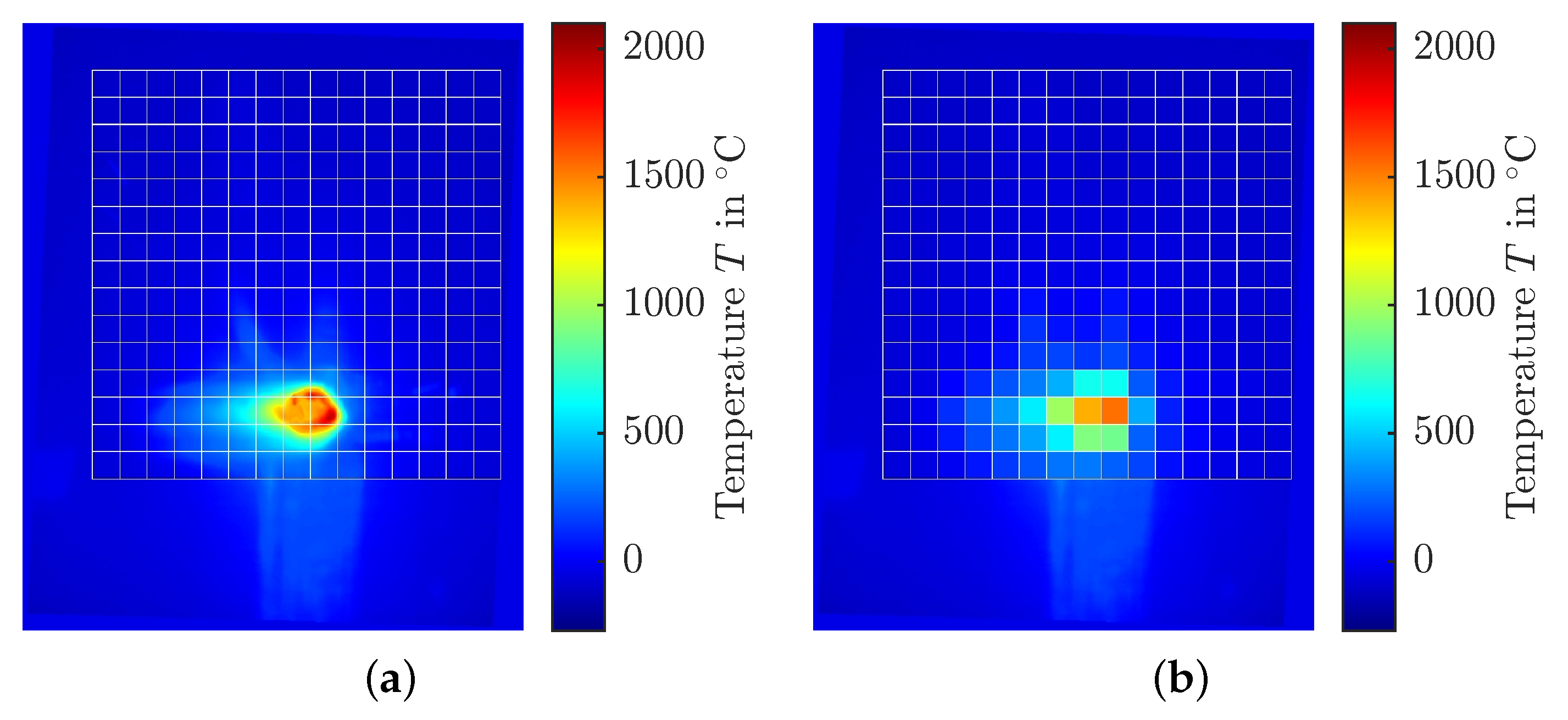
2.3. Measurement Data Processing

Proportionally to the radiance incident on the camera detector elements L cam , a voltage is generated in the detector elements, which is measured by the evaluation electronics and output as quantized digital count U D . Due to the manufacturer’s radiometric calibration, the relationship between the digital value U D and the temperature of a blackbody radiator ( ε = 1 ) is known. Since there are no blackbody radiators in the real applications, the influence of emissivity must be taken into account:
L cam = ε L obj ( T obj ) + ( 1 ε ) L amb ( T amb )
where L denotes the radiance captured by the camera L cam , by the object L obj or by the reflected ambient L amb depending on their corresponding temperature T. The emissivity ε takes values between 0 and 1 for real objects. Due to the protective measures described in Section 2.1, the used filters reduce the radiance beaming into the camera. This leads to an extended form of Equation (1):
L cam = τ ε L obj ( T obj ) + ( 1 ε ) L amb ( T amb ) + ( 1 τ ) L filter ( T filter )
where L filter denotes the self-radiation of the filter depending on its temperature T filter . To compensate for this effect, the transmittances of the plastic film and the laser protection filter were measured in the laboratory. For this purpose, a comparative radiance measurement with and without the filter element was performed using a setup with an infrared calibrator. This allows Equation (2) to be solved for τ . The transmittance of the foil was determined as τ foil = 0.78 and transmittance of the filter as τ filter = 0.73 , resulting in a total transmittance of τ = τ foil · τ filter = 0.57 .
According to Equation (2), the emissivity ε of the measured object is also required for the quantitatively correct conversion of the measured radiance values into temperatures. Unfortunately, due to the phase change of the metallic material, the required emissivity changes in an unknown manner and is hard to determine by experiments [1,15]. One way to approximate the emissivity is to use the characteristic point of the solidification plateau [16,17]. The emissivity is scaled so that this plateau corresponds to the known melting point temperature of 316L (≈ 1400   C ). This scaling was performed using the data from the first weld bead. Based on this procedure, an emissivity of ε = 0.40 is used within the scope of this work.
The conversion of the radiance readings to the corresponding temperatures (according to Equation (2)) is the first post-processing step. For example, Figure 4 depicts the resultant temperature evolution in five pixels located at the first weld bead of the specimen showing the characteristic heating and cooling periods at different spatial instances. Figure 5 shows a resultant false color image for a time instance at the end of the fabrication. From Figure 4, it becomes apparent that implausible temperature values result in parts of the measurement. Firstly, a scattering around a temperature of approx. 1500 C can be observed between the rising and falling slopes of the individual curves. This can be explained by the phase change of the metallic material and the changing emissivity as a consequence thereof, resulting in a too low temperature value in the liquid phase (melt pool) [17]. Secondly, there is a changing characteristic of the cooling rate below 225 C . In this case, the object temperature falls below the lower end of the calibrated temperature range of the infrared camera. An exclusion of such values would result in an insufficient amount of remaining data due to the spatial dependencies causing an ill-conditioned estimation problem in the following modeling step (see Section 3). Hence, it was decided to correct the lower temperature range by replacing the values below ambient temperature by a value of 26.6   C to get plausible output values in this range.
To correct the effects of the camera orientation, a geometric transformation of the image coordinate system was performed by point matching. To receive data suitable for system identification, appropriate resolutions of the temporally and spatially discretized data were selected. Due to large gradients of the dependent variable, the sampling time of Δ t = 1 / f s = 1 / 300 s was kept for identification resulting in N k = 14,000 time instances. The spatial resolution was chosen to be Δ x = 2 m m corresponding to the laser spot size resulting in a N s 1 × N s 2 dimensional grid with N s 1 = N s 2 = 15 . For example, Figure 6 shows the spatial discretization for one time instance in a false color image where the measured temperature in each grid cell is averaged.
In order to obtain the laser power input data, the trajectory of the laser was reconstructed from the temperature profile. The laser power was assumed to be uniformly distributed over the laser spot size which was confirmed by a caustic measurement. The resultant thermal evolution in one point together with the excitation signal is shown in Figure 7. The triangle shape of the input signal progress, which can be seen from Figure 7a is a consequence of the spatial downsampling. In Figure 7b, the reheating related to the subsequent deposition of further tracks can be observed.

3. Spatio Temporal Identification Fundamentals

In this section, the modeling approach and estimation procedure are described. In order to perform predictions based on a partial differential equation (PDE) model, the parameters of the model have to be known. As they are frequently hardly (or even not at all) a priori known, system identification techniques extended to the consideration of spatio-temporal dynamics can be used. In system identification, the behavior of a system is identified by measuring the response of the plant y R to an excitation signal u R . Based on the acquired data set D = { y ( k ) , u ( k ) } k = 1 N k with N k elements at the respective discrete time instances k, the aim is to find the unknown functional relationship:
y ( k ) = f ( x ( k ) ) + v ( k ) , k = 1 , , N k
where x ( k ) = [ y ( k 1 ) , , y ( k n y ) , u ( k 1 ) , , u ( k n u ) ] R n y + n u contains delayed values of the measured system output and the input. Note, possible dead times are dropped for brevity. The term v ( k ) is assumed to be independent and identically distributed noise with zero mean and finite variance σ 2 . The function f : R n R represents the system behavior to be modeled. For distributed systems, Equation (3) is extended to
y ( k , s ) = f ( x ( k , s ) ) + v ( k , s ) , k = 1 , , N k , s = 1 , , N s
with the (discrete) spatial domain s of arbitrary dimension. The choice of f can either be done based on physical insights or by using data-based approaches known from statistical learning (see, e.g., [18,19,20]). The former is preferred in this contribution.

3.1. Considered Model

In this contribution, the Finite Difference (FD) method is used in a rectangular spatial domain to discretize the partial derivatives of the governing PDE. To keep things simple, the following explanations are stated for a one-dimensional spatial domain. However, the approaches can be extended to the multidimensional case. We start from the well-known heat conduction equation (assuming no mass transfer or radiation as well as an isotropic and homogenous material)
T ( t , x ) t κ 1 2 T ( t , x ) x 2 = κ 2 u ( t , x )
where T denotes temperature, t and x continuous time and space, respectively. κ 1 and κ 2 are model coefficients containing the density, specific heat capacity, thermal conductivity, and absorbed thermal flux. u describes the input heat. To approximate the partial derivatives in Equation (5), the central differences
T ( t , x ) t k , s = T k + 1 , s T k , s Δ t
and
2 T ( t , x ) x 2 k , s = T k , s 1 2 T k , s + T k , s + 1 Δ x 2 ,
with the discrete time k = t k / Δ t Z + and the discrete space s = x s / Δ x Z , are used. Δ t is the sampling time and Δ x the spatial sampling distance. With Equations (6) and (7), the solution of Equation (5) can be approximated at the instance ( k , s ) using the difference equation
T k + 1 , s = a 1 , 1 T k , s 1 + a 1 , 0 T k , s + a 1 , 1 T k , s + 1 + b 1 , 0 u k , s .
In this case, a 1 , 1 = a 1 , 1 = κ 1 Δ t Δ x 2 , a 1 , 0 = 1 2 κ 1 Δ t Δ x 2 , and b 1 , 0 = κ 2 Δ t .
The generalized form of Equation (8) is given by
y k , s = ( i k , i s ) M y a i k , i s y ( k i k , s i s ) + ( j k , j s ) M u b j k , j s u ( k j k , s j s ) + v ( k , s )
where y ( k i k , s i s ) R and u ( k j k , s j s ) R are shifted versions of the output and input, respectively, a i k , i s R and b j k , j s R are the corresponding parameters, and an additional noise term v ( k , s ) is incorporated [21,22]. M y and M u define the spatial and temporal horizon of the output and the input, respectively, contributing to the dynamics of the output at instances ( k , s ) . For instance, for a two-dimensional system described by Equation (9), M y and M u are defined as subsets of the two-dimensional space, which include the indices of the coefficients of input and output terms in the difference equation. For instance, considering the discretized heat conduction Equation (8), the index sets M y and M u (given in Figure 8) are defined as
M y = { ( i k , i s ) | ( 1 , 1 ) , ( 1 , 0 ) , ( 1 , 1 ) } , M u = { ( j k , j s ) | ( 1 , 0 ) }
indicating the temporally and spatially shifted inputs and outputs required for calculating the output at instance ( k , s ) . By introduction of the temporal and spatial shift operators q k and q s , Equation (9) can be written in transfer function form:
y k , s = B ( q k , q s ) A ( q k , q s ) u ( k , s ) + H ( q k , q s ) e ( k , s )
where
A ( q k , q s ) = 1 + ( i k , i s ) M y a i k , i s q k i k q s i s B ( q k , q s ) = ( j k , j s ) M u b j k , j s q k j k q s j s
define the plant transfer function and H ( q k , q s ) defines the noise transfer function. If H ( q k , q s ) = 1 A ( q k , q s ) and e ( k , s ) represents a white noise signal, Equation (11) results in the so-called AutoRegressive with eXogenous input (ARX) model. The operators q k i k and q s i s introduce a shift of i k in the temporal and i s in the spatial domain (i.e., q k i k q s i s y ( k , s ) = y ( k i k , s i s ) ).
In order to obtain a more realistic noise assumption, the so-called Output Error (OE) model can be used. In this case, H ( q k , q s ) = 1 such that the noise is assumed to disturb the process additively at the output. Furthermore, in the OE model, the denominator of the plant transfer function is denoted as F ( q k , q s ) resulting in:
y k , s = B ( q k , q s ) F ( q k , q s ) u ( k , s ) + e ( k , s )
Note, as the noise model of the output error model does not include the process denominator dynamics 1 / A ( q k , q s ) , it is nonlinear in its parameters (see, e.g., [23]), and thus, much harder to estimate (cf. Section 3.3).

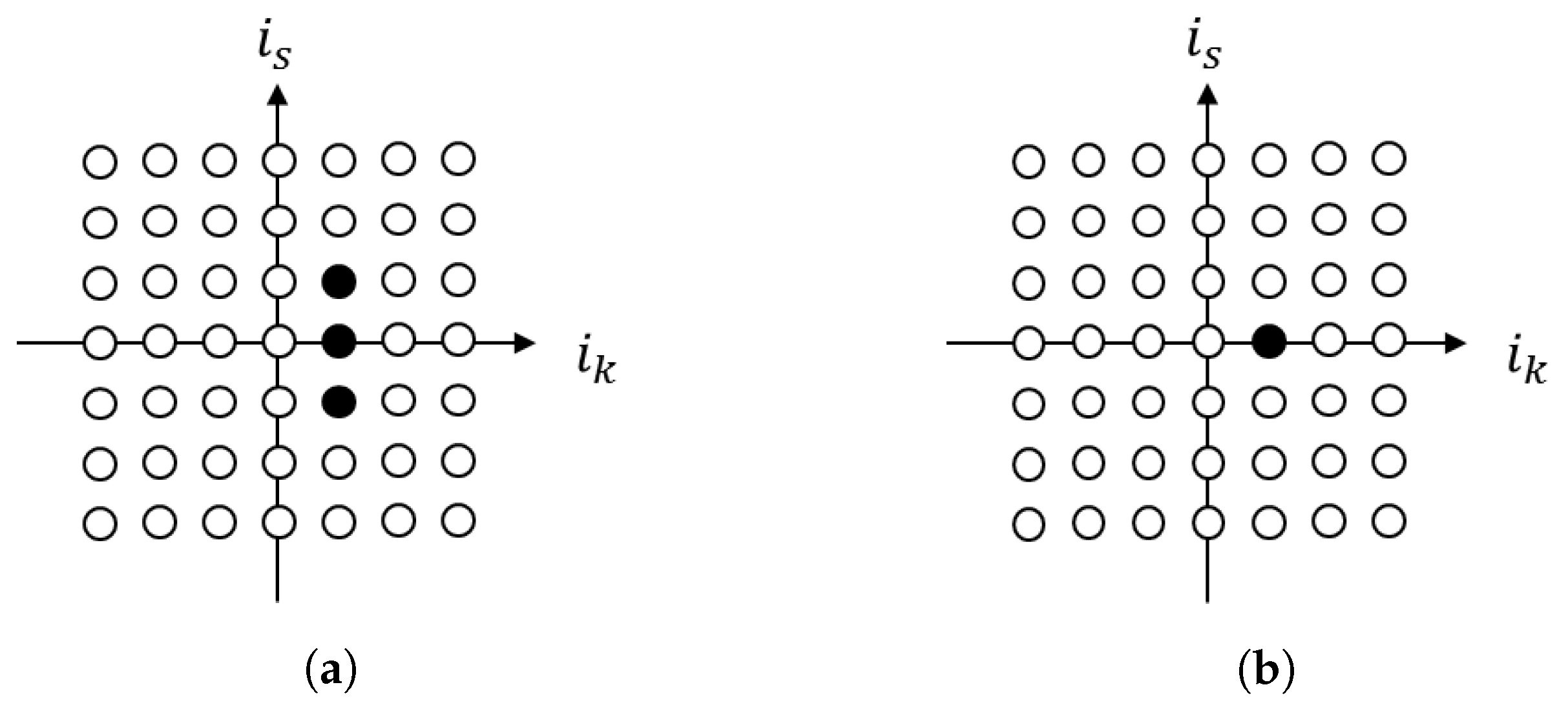
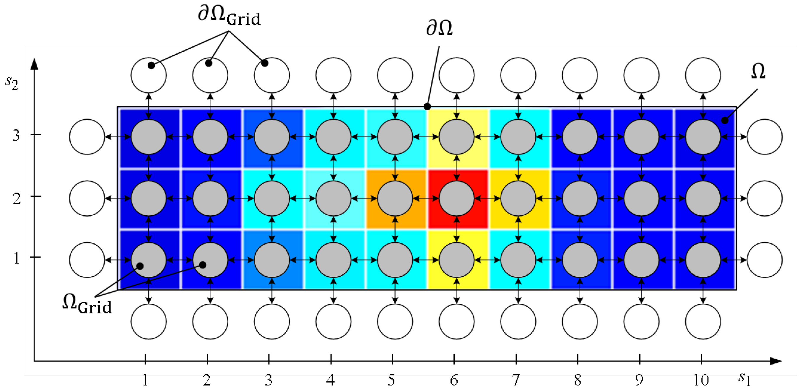
3.2. Spatial Discretization and Boundary Conditions

The approximation of a distributed system has to be restricted to a well-defined spatial domain. In this contribution, a grid partitioning of the spatial domain Ω = { x | r 1 < x < r 2 } R within the bounds r 1 and r 2 is considered, defined by
Ω Grid = { x Ω | x = r 1 + s Δ x , s Z } Ω .
In order to get a unique solution to a PDE, the initial states as well as the boundary conditions have to be specified. Common choices of boundary conditions are Dirichlet or Neumann conditions [24]. The former specifies the values that the solution of the PDE has to take along the boundary Ω of the spatial domain
y ( t , x ) = ϕ ( t , x ) x Ω ,
with known function ϕ ( t , x ) on Ω , whereas the latter imposes values of the derivative of the solution
y ( t , x ) n = ϕ ( t , x ) x Ω
where n denotes the normal vector to the boundary Ω . In this contribution, y ( t , x ) = 0 and y ( t , x ) / n = 0 are investigated. Furthermore, the initial states are assumed to be zero as well which is a common way in lumped system identification [25]. Figure 9 shows an exemplary grid partitioning for a weld bead together with the bounds in the two-dimensional spatial domain where the boundary conditions are defined on the fictional grid points Ω Grid . In Figure 10, the partitioning for the complete layer, as considered in this contribution (cf. Section 3.5), is illustrated.

3.3. Identification Approach

Once the initial states and considered spatial domain as well as the model structure by means of M y and M u are properly selected, the unknown coefficients of the model can be estimated within the Prediction Error Minimization (PEM) framework. In this contribution, a basic least squares approach introduced in [21] is used for ARX model identification and compared with a nonlinear optimization of the simulation error to obtain an OE model.
Introducing
φ ( k , s ) = y ( k i k , s i s ) u ( k j k , s j s ) ( i k , i s ) M y , ( j k , j s ) M u R n p ,
where n p = | M y | + | M u | , and the parameter vector
θ = a i k , i s b j k , j s ( i k , i s ) M y , ( j k , j s ) M u R n p ,
Equation (9) can be written in its linear regression form
y ( k , s ) = φ ( k , s ) θ + v ( k , s ) .
The predicted output of the model is given by
y ^ ( k , s ) = φ ( k , s ) θ ,
such that the prediction error ϵ ( k , s ) = y ( k , s ) y ^ ( k , s ) can be calculated. For a given input-output data set D R N k × N s the unknown parameters (18) can be estimated by minimizing a quadratic cost function
J ( θ , ϵ ) = 1 N k N s k = 1 N k s = 1 N s ϵ 2 ( k , s , θ ) .
In case of the ARX model, the least squares estimator can be used where the parameter estimates are obtained as
θ ^ LS = 1 N k N s k = 1 N k s = 1 N s φ ( k , s ) φ ( k , s ) 1 1 N k N s k = 1 N k s = 1 N s φ ( k , s ) y ( k , s ) .
In case of output error model identification, the prediction error ϵ in Equation (21) is calculated using the simulated output y ^ ( k , s ) = B ^ ( q k , q s ) F ^ ( q k , q s ) u ( k , s ) and the minimization of Equation (21) is done using nonlinear optimization. In this work, the trust region reflective method implemented in Matlab’s optimization toolbox is used where the solution of Equation (22) is used to initialize B ^ ( q k , q s ) and F ^ ( q k , q s ) .

3.4. Model Validation

In order to assess the resultant model, a visual inspection of the model predictions compared to the measured values of the temperature will be done. Furthermore, the following quantitative evaluation criteria are considered for model validation: (1) the Root Mean Square Error (RMSE) given by
RMSE = 1 N k N s k = 1 N k s = 1 N s y ( k , s ) y ^ ( k , s ) 2
and (2) the Best Fit Rate (BFR) given by
BFR = 100 % · max 1 k = 1 N k s = 1 N s y ( k , s ) y ^ ( k , s ) 2 k = 1 N k s = 1 N s y ( k , s ) y ¯ ( k , s ) 2 , 0
with y ¯ ( k , s ) being the mean value of the output.

3.5. 2D Thermal Model

For the sake of completeness, the considered model is given in the two-dimensional spatial domain as follows:
y k , s 1 , s 2 = ( i k , i s 1 , i s 2 ) M y a i k , i s 1 , i s 2 y ( k i k , s 1 i s 1 , s 2 i s 2 ) + ( j k , j s 1 , j s 2 ) M u b j k , j s 1 , j s 2 u ( k j k , s 1 j s 1 , s 2 j s 2 ) + v ( k , s 1 , s 2 )
with
M y = { ( i k , i s 1 , i s 2 ) | ( 1 , 0 , 0 ) , ( 1 , 1 , 0 ) , ( 1 , 1 , 0 ) , ( 1 , 0 , 1 ) , ( 1 , 0 , 1 ) } , M u = { ( j k , j s 1 , j s 2 ) | ( 1 , 0 , 0 ) } .
The data set is given by
D = { y ( k , s 1 , s 2 ) , u ( k , s 1 , s 2 ) R | k = 1 , , N k , s 1 = 1 , , N s 1 , s 2 = 1 , , N s 2 } ,
with N k = 14,000 and N s 1 = N s 2 .

4. Results and Discussion

In this section, the modeling approaches introduced in Section 3 are utilized in order to obtain mathematical models of the temperature evolution during the LMD process. For this, single tracks of the layer are considered firstly enabling an isolated examination and assessment of the modeling approaches where the inter-track dynamics and reheating effects are neglected. In a second consideration, the modeling approaches are examined on the whole layer experiment. Each model is given by Equations (25) and (26), with the measured temperature as output variable y k , s 1 , s 2 and the laser power as input u k , s 1 , s 2 . The model parameters are estimated using both ARX and OE configuration. The results (predicted values and evaluation criteria) reported in this section are based on the simulated output, i.e., the output is calculated based on the given input value and previous predictions of the output (OE configuration), imposing higher requirements on the model performances. As boundary conditions, Dirichlet conditions with ϕ ( k , s 1 , s 2 ) = 0 s 1 , s 2 Ω Grid and Neumann conditions with ϕ ( k , s 1 , s 2 ) = 0 s 1 , s 2 Ω Grid were tested and compared. The results given in the following subsections are limited to the use of Dirichlet conditions as they are slightly better.

4.1. Single Track Case

The results shown in this section are obtained when data corresponding to the spatial and time instances of welding the second track are used for model training. In order to validate the models on unseen data, the spatial and time instances corresponding to the welding of the fourth track are used. To account for the influences of the adjacent tracks, these are also included in the data sets, resulting in D t = { y ( k , s 1 , s 2 ) , u ( k , s 1 , s 2 ) D | k = 1001 , , 2000 , s 1 = 1 , , 15 , s 2 = 2 , , 4 } for training and D v = { y ( k , s 1 , s 2 ) , u ( k , s 1 , s 2 ) D | k = 3001 , , 4000 , s 1 = 1 , , 15 , s 2 = 4 , , 6 } for validation. Figure 11 illustrates the used grid, i.e., the considered spatial instances, for the training data. Note, a slight error may be obtained due to the used boundary conditions. However, as the adjacent tracks are also considered, the virtual boundary is not restricted to the geometrical boundary of the second weld bead and the measured values are used instead. The resultant performance criteria are summarized in Table 2. The estimated model coefficients are given in Table 3. From Table 2, it becomes apparent that a considerably better performance can be obtained if the model is trained in output error configuration. More particular, the low BFR value for the ARX model indicates that this modeling assumption is not suitable to obtain an adequate simulation model useful for the process under consideration. With respect to the estimated model coefficients given in Table 3, the estimated values of the OE model are one order of magnitude greater than the ones obtained for the ARX model despite for a 1 , 0 , 0 . More critically, the estimated value of a 1 , 0 , 1 is positive. From a physical point of view, all parameters corresponding to shifted versions of the output should have negative values. In addition, parameters being the spatially counterpart of one another should have similar values which is the case for the OE model.
Figure 12 shows the corresponding observed versus predicted plots for the models. As indicated by the performance criteria in Table 2, the ARX model is not capable to predict the correct response values in a simulation setting. This is confirmed by the simulation results depict in Figure 13a,b for one spatial instance. In fact, the model (25) represents a superposition of spatially distributed transfer functions characterized by their individual parameters a i k , i s 1 , i s 2 and the b parameter. While transfer functions of each spatial location with negative a parameter contribute a positive response value to the model output, the one with positive sign yield an inverse response behavior resulting in this unwanted aggregated model response. For the OE model, the scattering around the ideal prediction is acceptable (cf. Figure 12c,d). Merely in the upper range of the output, a trend of underestimating to overestimating the response value becomes apparent. This also comes up when considering the simulated output in Figure 13c. Due to the chosen model structure, the model is restricted to non-changing monotonicity behavior and, as a consequence, tries to average the effects occurring in the upper temperature ranges. However, a much better model fit can be obtained compared to the ARX model identification. On the validation data, the OE model shows a comparable simulation performance as on the training data (cf., Figure 13d).

4.2. Multiple Tracks Case

In this section, the former results are generalized to the whole layer. Of course, the limitations of the models stated before continue to apply. However, it is of great interest how the model behaves in this setting, as a lumped model would not be able to capture the inter-track relationship caused by the spatial dynamics. Therefore, for model training D t = { y ( k , s 1 , s 2 ) , u ( k , s 1 , s 2 ) D | k = 1 , , 10000, s 1 = 1 , , 15 , s 2 = 1 , , 15 } is used and the models are cross validated using D v = { y ( k , s 1 , s 2 ) , u ( k , s 1 , s 2 ) D | k = 10001, , 14000, s 1 = 1 , , 15 , s 2 = 1 , , 15 } . The corresponding grid partitioning has already been shown in Figure 10. The resulting performance criteria are summarized in Table 4. The estimated model coefficients are given in Table 5. Again, the ARX model is not capable to predict the temperature for the data at hand. Whereas, the OE model shows a moderate simulation performance regarding the evaluation criteria. Compared to the single track results, the BFR and RMSE on training data decrease while on validation data the RMSE increases and the BFR decreases. The simultaneous decrease of RMSE and BFR on training data seem counter-intuitive but can be explained by the changing properties of the considered data sets. The RMSE is the square root of the sum of squared residuals divided by N k · N s , therefore a measure of the variation not explained by the model. Thus, while the squared residuals increase just slightly considering the multiple tracks experiment, the amount of data compensates for that effect resulting in a lower RMSE value, i.e., the predictions are closer to the observed values on average. On the other hand, the BFR measures the percentage of variance of y explained by the model, i.e., how close the predictions are to the observed values. This effect becomes clear taking a look on the observed versus predicted values in Figure 14. Basically, similar patterns as for the single track consideration can be seen. The ARX model tends to underestimate the temperature evolution, which can be explained following the explanations given in the previous section and considering the estimated model parameters in Table 5. For the OE model, a wider scattering around the ideal black dashed line confirm the lower BFR value. But most of the predictions seem as close to the observed values as for the single track experiment confirming the lower RMSE value on the training data. On the other hand, the predictions on the validation data set seem slightly biased, i.e., the model tends to underestimate the temperature. However, the qualitative progression of the temperature evolution is captured by the model.
Figure 15a,b show the simulation results of the OE model for different spatial instances on the training data. Figure 15c shows the results for one spatial instance on the validation data. Note that there are changing x axis from Figure 15a–c. Compared to the single track case, the resultant time series show multiple peaks due to pre- and reheating in the individual cells by the energy input of the laser into the surrounding ones. This effect can be well predicted by the model. Solely with ongoing progressive duration of the experiment, a slight misalignment of the predicted and observed peaks occur. To be more precise, cells corresponding to locations produced at later time instances show a slight offset of the observed temperature after the energy input, which is not captured by the model. Additionally, the model underestimates the main peaks on the validation data which has been already observed in Figure 14d. Apparently, the former effect can not simply be explained by the changing initial conditions of spatially interconnected cells taken into account by the model. Probably, this effect can be dealt with by incorporating a parameter varying offset term in the model. Furthermore, note that there are multiple input peaks in each spatial instance shown in Figure 15. This is caused by the misalignment of the reconstructed input (or melt pool) trajectory relative to the grid chosen for spatial discretization. The maximum value of 1 k W of the laser power will only be reached when the laser track goes through the center of the grid cells. If there is a relative shift, the laser power is additionally distributed to adjacent tracks.

4.3. Discussion

As already discussed in the previous subsections, the investigated modeling approaches show promising results, but are not capable to account for each phenomena contained in the data. From the single track case, it becomes evident that the changing characteristics of the temperature evolution in the upper range can not be captured sufficiently by the model. In fact, the observed behavior of the temperature evolution in this range is based on the globally fixed emissivity ε at the solidification plateau for the conversion of radiance to temperature (see Section 2.3) and thus is limiting the plausibility of the results from a physical perspective. As a recent work with a multispectral sensing approach indicates [26], the emissivity can vary significantly during the build process. In particular, the phase transition in the melt pool and the progressing oxidation of the workpiece influence the optical surface properties (and thus the emissivity). The temperature readings are therefore more likely to be correct on the falling slope of the temperature profile, but at other positions the temperature output of the camera is only an apparent temperature. It will be part of future work to integrate a visual camera in the process in order to be able to observe effects influencing the emissivity (such as oxidation) and subsequently adapt the emissivity spatially and temporally resolved. For two reasons, the modeling approach presented here can still be used to control the process in the future. At first, the temperature gradients during cooling, which are well represented by the model, are most important for the subsequent mechanical properties of the workpiece. Secondly, the absolute temperature may not be as relevant for a later process control as step changes of the temperature or temperature gradients. In order to deal with the changing monotonicity in areas of phase transition, the model structure has to be adapted, at least by allowing for higher order dynamics in the temporal domain which will be investigated in future work. To deal with the increasing temperature offset observed in the multiple tracks consideration, a linear parameter varying model structure could be assumed as proposed by [27]. However, altogether an adequate simulation performance is already obtained although the used model greatly simplifies the occurring physical phenomena of the LMD process. Of course, the non-contacting thermal measurement is restricted to surface temperatures. However, from a control-oriented perspective, the proposed model would drastically reduce the computational burden for a layer-wise control update while preserving the consideration of inter-track dynamics. From a modeling point of view, the next step would be the consideration of inter-layer dynamics, at least by predicting the initial and boundary conditions for a subsequent layer, which will be part of future work.

5. Conclusions

In this work, spatio-temporal measurements of the temperature evolution were conducted by using an infrared camera in order to model the thermal characteristics of the LMD process by using data-driven approaches. A complete pre-processing scheme is proposed enabling the generation of data suitable for identification of spatio-temporal models. As models, the class of spatio-temporal input–output models represented by partial difference equations are considered. Different model classes—namely, ARX and OE—were investigated accounting for different noise assumptions. The model structure was derived from the general heat conduction equation. In order to enable isolated investigations, the single track as well as multiple tracks case was considered. It was shown that:
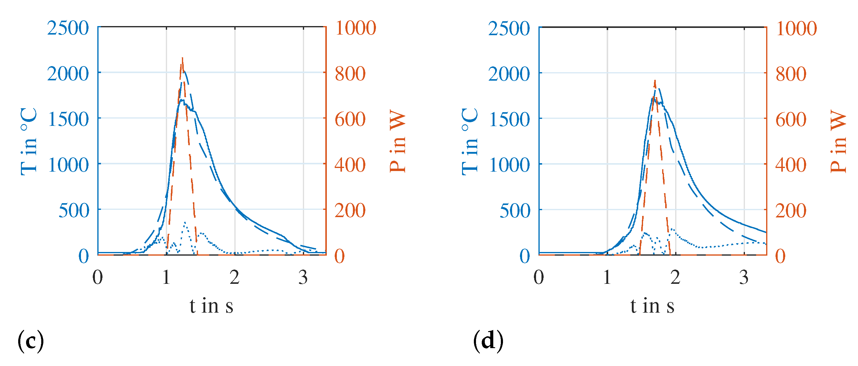
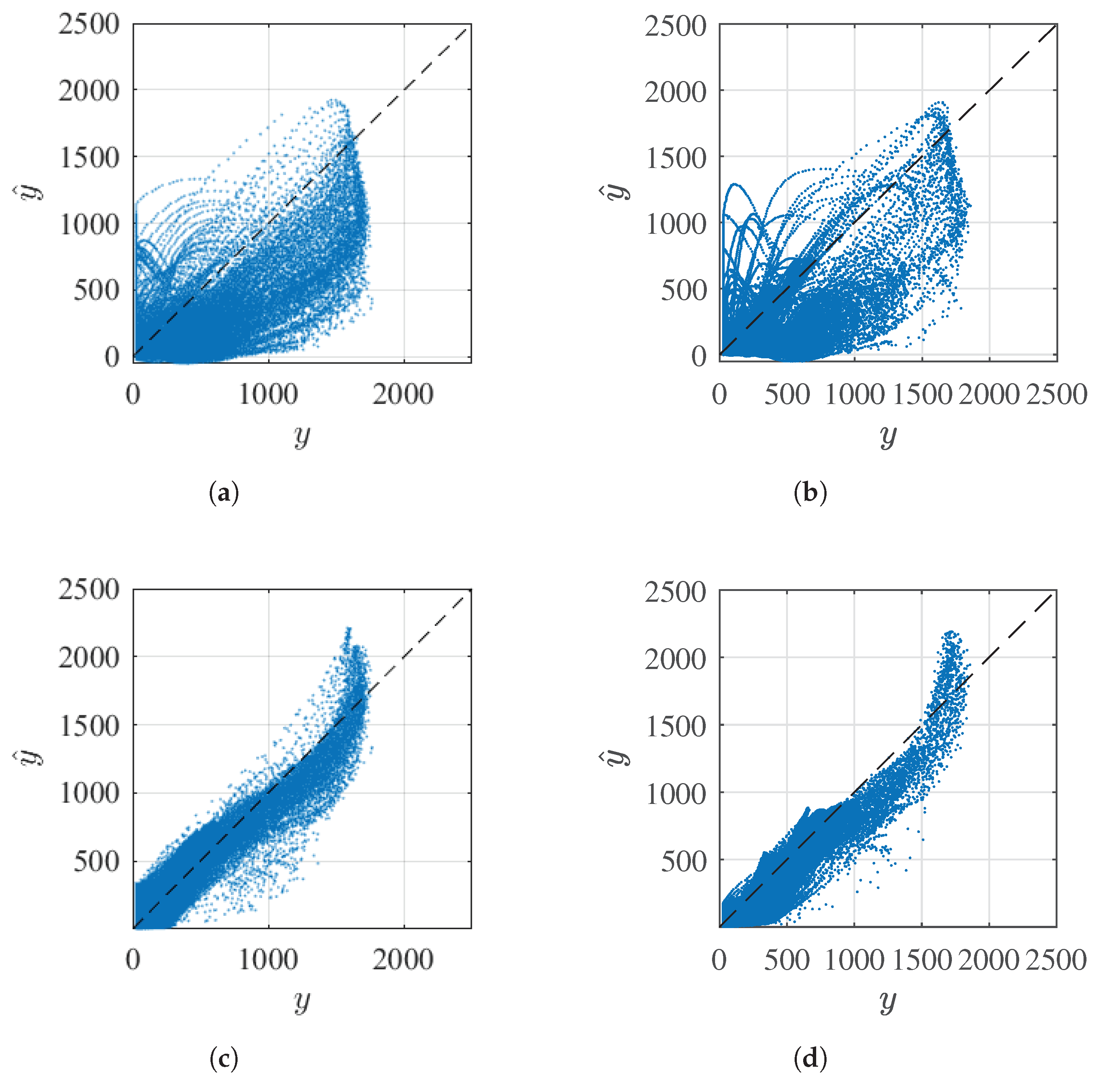
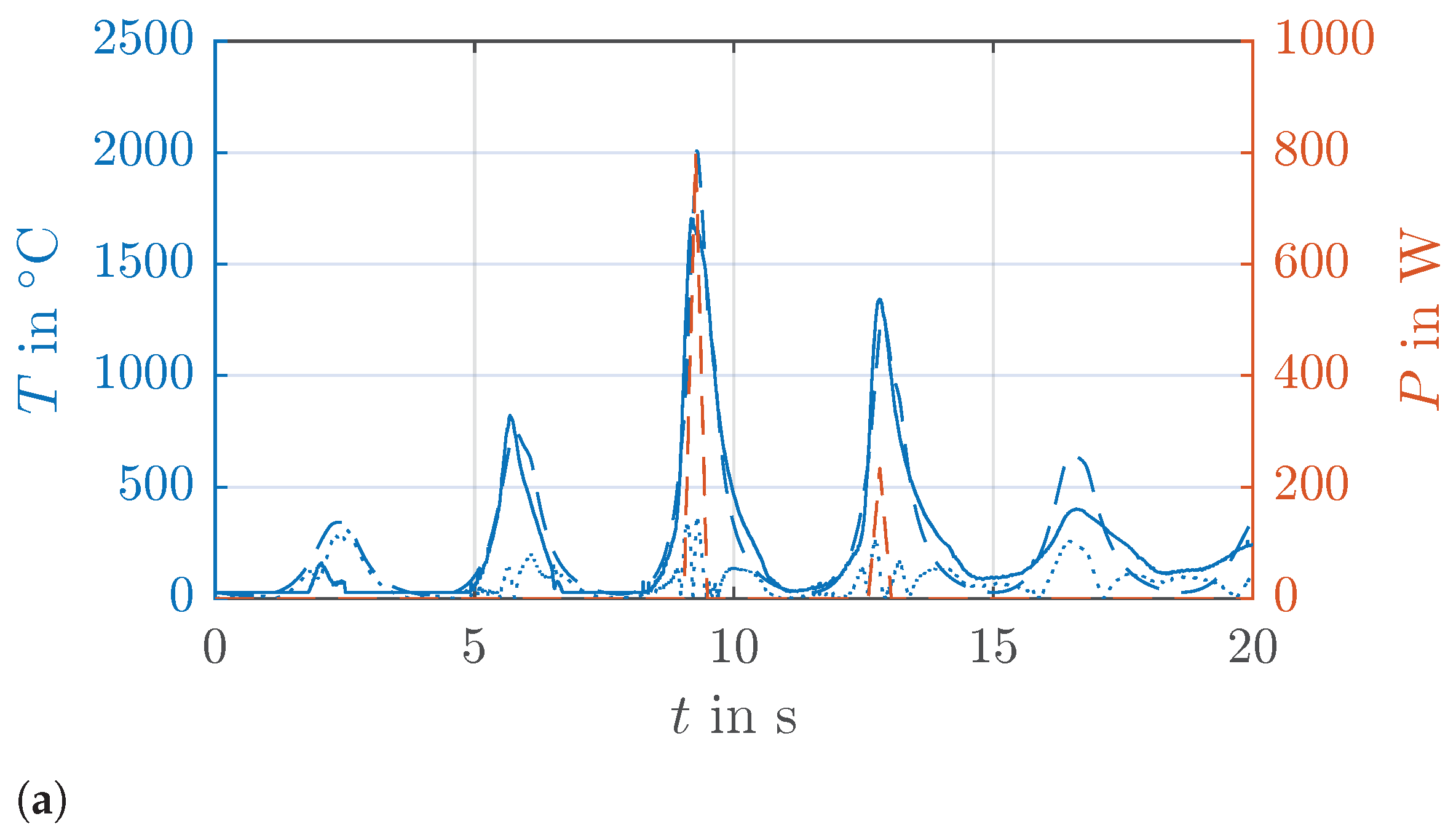
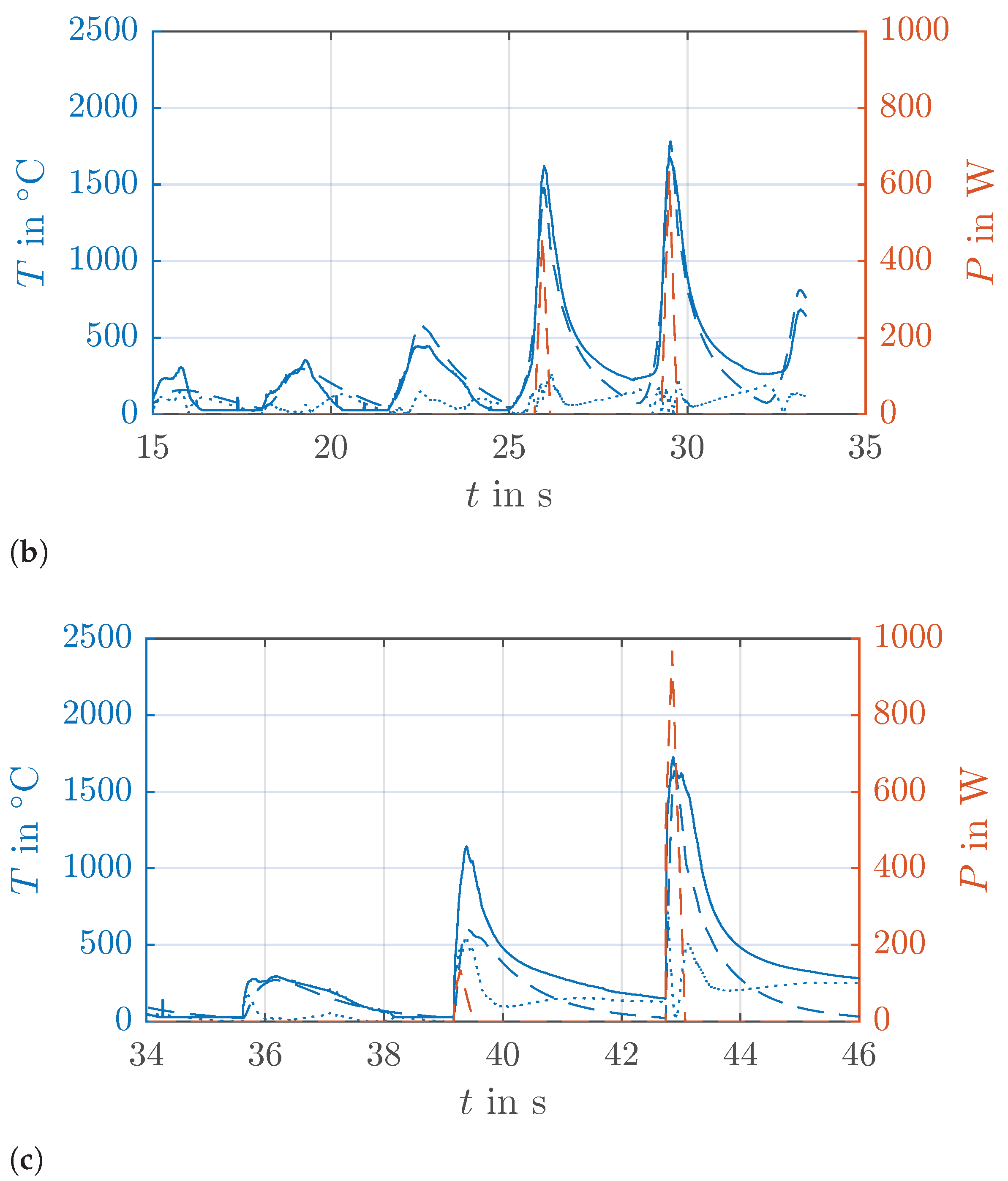
  • The ARX model assumption yields insufficient results when used for simulation purposes, whereas, acceptable results can be obtained using OE models.
  • A significant change in the thermal behavior measured with the IR camera in areas of phase transitions results when assuming a globally fixed emissivity.
  • The model structure derived from the general heat conduction equation restricts the obtained results to first order temporal dynamics resulting in a mismatch of the predictions in periods of phase transitions.
  • Pre- and reheating effects can be mostly predicted by the resultant model when considering the multiple tracks case. However, a changing offset of the observed temperature with ongoing progressive duration of the experiment could not be described by incorporation of the spatial dynamics into the model so far.

Author Contributions

Conceptualization, M.K. and M.N.; data curation, S.S. and M.N.; formal analysis, M.K.; investigation, M.K.; methodology, M.K. and S.S.; resources, M.K.; software, M.K. and M.N.; supervision, A.K.; validation, M.K.; visualization, M.K. and S.S.; writing—original draft, M.K. and S.S.; writing—review and editing, M.N. and A.K. All authors have read and agreed to the published version of the manuscript.

Funding

Part of the work was supported by the research program “future” of the University of Kassel.

Institutional Review Board Statement

Not applicable.

Informed Consent Statement

Not applicable.

Data Availability Statement

The data is available from the authors.

Acknowledgments

The authors would like to thank the Department of Cutting and Joining Technology (tff) of the University of Kassel for providing the LBM facility and the supervision during the experiments, especially Stefan Böhm and Niklas Sommer.

Conflicts of Interest

The authors declare no conflict of interest.

Sample Availability

Not applicable.

Abbreviations

The following abbreviations are used in this manuscript:
AMAdditive manufacturing
ARXAutoregressive with exogenous input
BFRBest fit rate
CFDComputational fluid dynamics
FDFinite difference
FEMFinite element method
IRInfrared
LMDLaser metal deposition
MIMOMulti-input multi-output
MWIRMid-wave infrared
OEOutput error
PDEPartial difference equation
PEMPrediction error minimization
PIDProportional-integral-derivative
RMSERoot mean squared error

References

  1. Thompson, S.M.; Bian, L.; Shamsaei, N.; Yadollahi, A. An overview of Direct Laser Deposition for additive manufacturing; Part I: Transport phenomena, modeling and diagnostics. Addit. Manuf. 2015, 8, 36–62. [Google Scholar] [CrossRef]
  2. Shamsaei, N.; Yadollahi, A.; Bian, L.; Thompson, S.M. An overview of Direct Laser Deposition for additive manufacturing; Part II: Mechanical behavior, process parameter optimization and control. Addit. Manuf. 2015, 8, 12–35. [Google Scholar] [CrossRef]
  3. Farshidianfar, M.H.; Khajepour, A.; Gerlich, A.P. Effect of real-time cooling rate on microstructure in laser additive manufacturing. J. Mater. Process. Technol. 2016, 231, 468–478. [Google Scholar] [CrossRef]
  4. Salehi, D.; Brandt, M. Melt pool temperature control using LabVIEW in Nd: YAG laser blown powder cladding process. Int. J. Adv. Manuf. Technol. 2006, 29, 273–278. [Google Scholar] [CrossRef]
  5. Tang, L.; Landers, R.G. Melt pool temperature modeling and control for laser metal deposition processes. In Proceedings of the 2009 American Control Conference (ACC), IEEE, St. Louis, MI, USA, 10–12 June 2009; pp. 4791–4796. [Google Scholar]
  6. Tang, L.; Landers, R.G. Melt pool temperature control for laser metal deposition processes—Part I: Online temperature control. J. Manuf. Sci. Eng. 2010, 132, 011010. [Google Scholar] [CrossRef]
  7. Tang, L.; Landers, R.G. Melt pool temperature control for laser metal deposition processes—Part II: Layer-to-layer temperature control. J. Manuf. Sci. Eng. 2010, 132, 011011. [Google Scholar] [CrossRef] [Green Version]
  8. Song, L.; Mazumder, J. Feedback control of melt pool temperature during laser cladding process. IEEE Trans. Control. Syst. Technol. 2010, 19, 1349–1356. [Google Scholar] [CrossRef]
  9. Song, L.; Bagavath-Singh, V.; Dutta, B.; Mazumder, J. Control of melt pool temperature and deposition height during direct metal deposition process. Int. J. Adv. Manuf. Technol. 2012, 58, 247–256. [Google Scholar] [CrossRef]
  10. Wang, H.; Liu, W.; Tang, Z.; Wang, Y.; Mei, X.; Saleheen, K.M.; Wang, Z.; Zhang, H. Review on adaptive control of laser-directed energy deposition. Opt. Eng. 2020, 59, 070901. [Google Scholar] [CrossRef]
  11. Sammons, P.M.; Bristow, D.A.; Landers, R.G. Two-dimensional modeling and system identification of the laser metal deposition process. J. Dyn. Syst. Meas. Control. 2019, 141. [Google Scholar] [CrossRef]
  12. Cao, X.; Ayalew, B. Control-oriented MIMO modeling of laser-aided powder deposition processes. In Proceedings of the 2015 American Control Conference (ACC), Chicago, IL, USA, 1–3 July 2015; pp. 3637–3642. [Google Scholar]
  13. Cao, X.; Ayalew, B. Multivariable predictive control of laser-aided powder deposition processes. In Proceedings of the 2015 American Control Conference (ACC), Chicago, IL, USA, 1–3 July 2015; pp. 3625–3630. [Google Scholar]
  14. Cao, X.; Ayalew, B. Robust multivariable predictive control for laser-aided powder deposition processes. J. Frankl. Inst. 2019, 356, 2505–2529. [Google Scholar] [CrossRef]
  15. Goett, G.; Kozakov, R.; Uhrlandt, D.; Schoepp, H.; Sperl, A. Emissivity and temperature determination on steel above the melting point. Weld. World 2013, 57, 595–602. [Google Scholar] [CrossRef]
  16. Lane, B.; Moylan, S.; Whitenton, E.P.; Ma, L. Thermographic measurements of the commercial laser powder bed fusion process at NIST. Rapid Prototyp. J. 2016, 22, 778–787. [Google Scholar] [CrossRef] [PubMed] [Green Version]
  17. Doubenskaia, M.; Pavlov, M.; Grigoriev, S.; Smurov, I. Definition of brightness temperature and restoration of true temperature in laser cladding using infrared camera. Surf. Coatings Technol. 2013, 220, 244–247. [Google Scholar] [CrossRef]
  18. Kahl, M.; Kroll, A.; Kästner, R.; Sofsky, M. Application of model selection methods for the identification of a dynamic boost pressure model. IFAC-Pap. 2015, 48, 829–834. [Google Scholar] [CrossRef]
  19. Kahl, M.; Kroll, A. Structure identification of dynamical takagi-sugeno fuzzy models by using lpv techniques. Arch. Data Sci. Ser. (Online First) 2018, 5, A19. [Google Scholar]
  20. Kahl, M.; Kroll, A. Extending Regularized Least Squares Support Vector Machines for Order Selection of Dynamical Takagi-Sugeno Models. IFAC-Pap. 2020, 53, 1182–1187. [Google Scholar] [CrossRef]
  21. Ali, M.; Chughtai, S.S.; Werner, H. Identification of spatially interconnected systems. In Proceedings of the 48th IEEE Conference on Decision and Control (CDC) held jointly with 28th Chinese Control Conference, Shanghai, China, 16–18 December 2009; pp. 7163–7168. [Google Scholar]
  22. Ali, M.; Chughtai, S.S.; Werner, H. Consistent identification of two-dimensional systems. In Proceedings of the 2010 American Control Conference, Baltimore, MD, USA, 30 June–2 July 2010; pp. 3464–3469. [Google Scholar]
  23. Nelles, O. Nonlinear System Identification: From Classical Approaches to Neural Networks, Fuzzy Models, and Gaussian Processes, 2nd ed.; Springer Nature: Berlin/Heidelberg, Germany, 2020. [Google Scholar]
  24. LeVeque, R.J. Finite Difference Methods for Ordinary and Partial Differential Equations: Steady-State and Time-Dependent Problems; SIAM: Philadelphia, PA, USA, 2007. [Google Scholar]
  25. Ljung, L. System Identification: Theory for the User, 2nd ed.; Prentice Hall PTR: Upper Saddle River, NJ, USA, 1999. [Google Scholar]
  26. Altenburg, S.J.; Scheuschner, N.; Gumenyuk, A.; Maierhofer, C. Towards the determination of real process temperatures in the LMD process by multispectral thermography. In Thermosense: Thermal Infrared Applications XLIII; International Society for Optics and Photonics: Bellingham, WA, USA, 2021; Volume 11743, p. 117430B. [Google Scholar]
  27. Ali, M.; Chughtai, S.S.; Werner, H. Identification of LPV models for spatially varying interconnected systems. In Proceedings of the 2010 American Control Conference (ACC), Baltimore, MD, USA, 30 June–2 July 2010; pp. 3889–3894. [Google Scholar]
Figure 1. Schematic of the experimental setup.
Metals 11 02050 g001
Figure 2. Camera setup during the LMD process. The protective enclosure is only opened for the photography of the setup.
Metals 11 02050 g002
Figure 3. Produced specimen.
Metals 11 02050 g003
Figure 4. Temperature evolution in five distinct points of the first weld bead.
Metals 11 02050 g004
Figure 5. Resultant false color image of the specimen for time instance at the end of the build process.
Metals 11 02050 g005
Figure 6. False color image with predefined grid before (a) and after (b) spatial downsampling at time instance k = 4000 .
Metals 11 02050 g006
Figure 7. Thermal evolution in one discrete point ( s 1 , s 2 ) = ( 7 , 2 ) after spatial downsampling. Left axis (blue): Measured temperature (solid line) and corrected temperature values (dashed line). Right axis (red): Corresponding laser power. (a) First 3 s of experiment; (b) Hole duration of experiment.
Metals 11 02050 g007
Figure 8. Illustration of required input and output lags (filled circles) for calculation of y ( k , s ) based on Equation (8) on two-dimensional lattice. (a) Index set M y ; (b) index set M u .
Metals 11 02050 g008
Figure 9. Illustration of spatial discretization for one weld bead.
Metals 11 02050 g009
Figure 10. Illustration of spatial discretization for one layer: (a) Schematic of specimen with grid, (b) corresponding false color image with grid.
Metals 11 02050 g010
Figure 11. Illustration of spatial discretization of training data for single track case: (a) Schematic of specimen with grid (white circles represent fictional boundary grid points), (b) corresponding false color image with grid.
Metals 11 02050 g011
Figure 12. y versus y ^ plots for single track case. (a) ARX model predictions on training data; (b) ARX model predictions on validation data; (c) OE model predictions on training data; (d) OE model predictions on validation data.
Metals 11 02050 g012
Figure 13. Time series for single track case at spatial instance ( s 1 , s 2 ) = ( 5 , 2 ) for both, training and validation data. Left axis (blue): Observed temperature y (solid line), predicted temperature y ^ (dashed line), and absolute value of residuals ϵ (dotted line). Right axis (red): Corresponding laser power. (a) ARX model, training data; (b) ARX model, validation data; (c) OE model, training data; (d) OE model, validation data.
Metals 11 02050 g013aMetals 11 02050 g013b
Figure 14. y versus y ^ plots for multiple tracks experiment. (a) ARX model predictions on training data; (b) ARX model predictions on validation data; (c) OE model predictions on training data; (d) OE model predictions on validation data.
Metals 11 02050 g014
Figure 15. Time series for multiple tracks case at spatial instances ( s 1 , s 2 ) = { ( 3 , 3 ) , ( 7 , 7 ) } on training and ( s 1 , s 2 ) = ( 12 , 12 ) on validation data. Left axis (blue): Observed temperature y (solid line), predicted temperature y ^ (dashed line), and absolute value of residual ϵ (dotted line). Right axis (red): Corresponding laser power. (a) Time series at spatial instance (3,3) on training data; (b) Time series at spatial instance (7,7) on training data; (c) Time series at spatial instance (12,12) on validation data.
Metals 11 02050 g015aMetals 11 02050 g015b
Table 1. Operating conditions.
Process/Operating ParameterValue/Setting
Laser power1000 W
Laser spot size~2 m m
Powder feed rate12 g   ·   min 1
Traverse speed10 mm   ·   s 1
Argon gas flow rate (carrier)20 L   ·   min 1
Argon gas flow rate (shielding)25 L   ·   min 1
Powder materialAISI 316 L
Powder size distribution50 μ m to 150 μ m
Number of tracks13
Length of each track25 m m
Hatch spacing2 m m
Scanning patternmono-directional
Table 2. Performance of ARX and OE models for simulation assessed for training and validation data, respectively, for single track case.
RMSE in C BFR in %RMSE in C BFR in %
(Training)(Training)(Validation)(Validation)
ARX325.4711.21343.847.76
OE126.2179.3796.6074.09
Table 3. Estimated model coefficients in single track case. Note, for brevity the same denotation of the parameters corresponding to shifted output values is used for both, ARX and OE case.
a 1 , 0 , 0 a 1 , 1 , 0 a 1 , 1 , 0 a 1 , 0 , 1 a 1 , 0 , 1 b 1 , 0 , 0
ARX−0.993−0.002−0.002−0.0090.0050.009
OE−0.871−0.051−0.041−0.026−0.0270.148
Table 4. Performance of ARX and OE models for simulation assessed for training and validation data, respectively, for multiple tracks case.
RMSE in C BFR in %RMSE in C BFR in %
(Training)(Training)(Validation)(Validation)
ARX159.1319.37211.490.83
OE69.6764.61115.1246.02
Table 5. Estimated model coefficients. Note, for brevity the same denotation of the parameters corresponding to shifted output values is used for both, ARX and OE case.
a 1 , 0 , 0 a 1 , 1 , 0 a 1 , 1 , 0 a 1 , 0 , 1 a 1 , 0 , 1 b 1 , 0 , 0
ARX−0.989−0.002−0.001−0.0100.0030.018
OE−0.902−0.019−0.016−0.029−0.0300.140
Publisher’s Note: MDPI stays neutral with regard to jurisdictional claims in published maps and institutional affiliations.

