Investigation of the Extrapolation Capability of an Artificial Neural Network Algorithm in Combination with Process Signals in Resistance Spot Welding of Advanced High-Strength Steels

Abstract

Resistance spot welding is an established joining process for the production of safety-relevant components in the automotive industry. Therefore, consecutive process monitoring is essential to meet the high quality requirements. Artificial neural networks can be used to evaluate the process parameters and signals, to ensure individual spot weld quality. The predictive accuracy of such algorithms depends on the provided training data set, and the prediction of untrained data is challenging. The aim of this paper was to investigate the extrapolation capability of a multi-layer perceptron model. That means, the predictive performance of the model was tested with data that clearly differed from the training data in terms of material and coating composition. Therefore, three multi-layer perceptron regression models were implemented to predict the nugget diameter from process data. The three models were able to predict the training datasets very well. The models, which were provided with features from the dynamic resistance curve predicted the new dataset better than the model with only process parameters. This study shows the beneficial influence of process signals on the predictive accuracy and robustness of artificial neural network algorithms. Especially, when predicting a data set from outside of the training space.

1. Introduction

Resistance spot welding (RSW) is an efficient and highly automated joining technology used in car manufacturing. A typical car body has up to 5000 resistance spot welds [1], with a varying number of joining partners, different materials, and different sheet thicknesses [2]. These variations, the high process speed, and the various sources of errors, such as gaps and improper component alignment [3], increase the process complexity [4]. This is also reflected in the rigorous testing efforts and the extensive destructive tests in mass production [3]. An automotive production line of high-volume models produces more than 7 million welds daily [5]. It is estimated that up to 20% of the spot welds are only made to ensure the component safety of welded assemblies [6]. Hence, reliable process monitoring is essential to save costs and limit production effort.

A welding power supply manufacturer developed real-time control approaches [7] that record the dynamic resistance (DR) curve for each spot weld and compare it with a previously determined optimal master data set. In case of deviations, the weld current is controlled [8] to keep the heat input constant for all welds. The final quality documentation of the process is carried out by the production personnel. For this purpose, destructive testing [8] is applied on random samples, to measure the geometrical attributes of the weld nugget. For example, it is necessary to ensure that the weld nugget is large enough and is formed across all joining planes [9], because of the significant influence on the mechanical properties of the welded joint [10]. In this case, the quality evaluation is largely dependent on the experience of the inspector and the inspection interval [8].

A digitalized solution that provides consistent results regarding the individual quality evaluation of spot welds is desirable; especially for safety-relevant components (e.g., car bodies) that require comprehensive documentation [11] to ensure the traceability of manufacturing failures [12]. In some disciplines, e.g., additive manufacturing, there have already been efforts made towards the individual documentation of component quality [13]. The aim is to evaluate the quality of an individual production step (additive manufacturing, welding, etc.) with the aid of sensors, algorithms, and simulations, in order to document, and finally, to certify it [14]. In particular, the growing trend of offering highly configurable products is driving the increase in manufacturing efforts [15]. To overcome this rise in complexity, artificial intelligence (AI) methods are suitable tools.

As data-driven approaches, AI algorithms are appropriate for predicting the RSW process [16]. They are able to model very complex and highly nonlinear relations [17]. The implementation and modelling of an algorithm represents the main effort, whereas the calculation of each weld spot can be done in real time [18]. Furthermore, AI algorithms can be used to leverage historical process data [19], in order to improve process parameter predictions. In contrast to empirical and statistical models, the AI models do not require any assumptions and prior knowledge about the physical phenomena of a context to be modelled. Commonly used AI algorithms include artificial neural networks (ANN) [20], decision trees [21], and support vector machines [20].

Literature Review

AI algorithms have already been used to reliably perform quality checks during manufacturing [22]. Afshari et al. [23] implemented an ANN based on process parameters to estimate the size of the weld nugget in the RSW of two-sheet joints. Subsequently, the authors compared the results with a finite element simulation and found that both, ANNs and simulations, were equivalent in terms of accuracy. Ahmed et al. [18] implemented a decision tree algorithm to predict the spot diameter from process parameters such as current, weld time, material, and coating. The authors trained the algorithm with the whole dataset and showed that the trained parameters were sufficient to predict the nugget diameter accurately. Arunchai et al. [24] implemented an ANN algorithm to predict the shear strength of aluminum RSW specimens from the following parameters: current, electrode force, welding time, and contact resistance. The algorithm was able to predict the shear strength accurately. The model was trained with 75% of the whole data set and tested with 25%. This so called ‘train–test split’ technique is used to evaluate the performance of an AI algorithm. The training dataset is used to fit the model, whereas the testing dataset is used to evaluate the accuracy. Panda et al. [20] implemented a support vector machine algorithm to predict the failure load of spot welded aluminum sheets. Martin et al. [25] used an ANN algorithm to evaluate the welding time, current, electrode force, and to predict the tensile shear strength of spot-welding joints of AISI 304.

The accuracy and robustness of models is dependent on the data provided for training. Wang et al. [17] examined the application of AI models in welding for monitoring and diagnosis purposes. They found that AI algorithms can predict the observed processes well, but can have large errors when extrapolating beyond the observation range. Zhou et al. [22] stated that most AI approaches lack generality and can only be applied in limited fields, where input data are sufficiently available. Fabry et al. [26] investigated the extrapolation capabilities of an ANN model at the edge of, and beyond, the trained parameter space. The authors found that high deviations from the original data often occurred. Therefore, they recommended only relying on the approximation of a previously trained ANN for areas inside the parameter space of the training dataset. Hence, the evaluation of unknown data, which are not part of training, is still challenging. A possible approach to improve the robustness is to include process signals. It can be assumed that the behavior of the process signals for different specimens and materials will, on average, be similar.

In their work, Boersch et al. [27] developed a decision tree algorithm for the prediction of weld spot diameters based on process data and features extracted from the DR curve. The authors segmented the curve and calculated different geometric and statistical features for every segment. This resulted in a highly accurate decision tree regression model for predicting the weld nugget size. Wan et al. [28] used an ANN to predict the size of weld nuggets during RSW of two-sheet joints. The authors were also able to achieve a high prediction accuracy by evaluating the DR. Lee et al. [29] implemented an AI algorithm to predict the electrode misalignment based on process parameters and the DR curve. The authors showed that AI models trained with features from the DR curve were able to predict data that differed slightly from the training data.

In the literature, authors predicted with a high accuracy target variables, such as nugget diameter and shear strength, mainly on the basis of process data obtained from lab environments. The conditions in industry differ from those in the laboratory. To transfer such AI models to real manufacturing, it is necessary to prove the robustness of the models. In this paper, weld nugget diameter was predicted from process parameters and signals using a multi-layer perceptron (MLP) regression algorithm. Moreover, the behavior of the AI model with a new data set, which was not part of the training, was tested, and the extrapolation ability of the model was investigated.

2. Materials and Methods

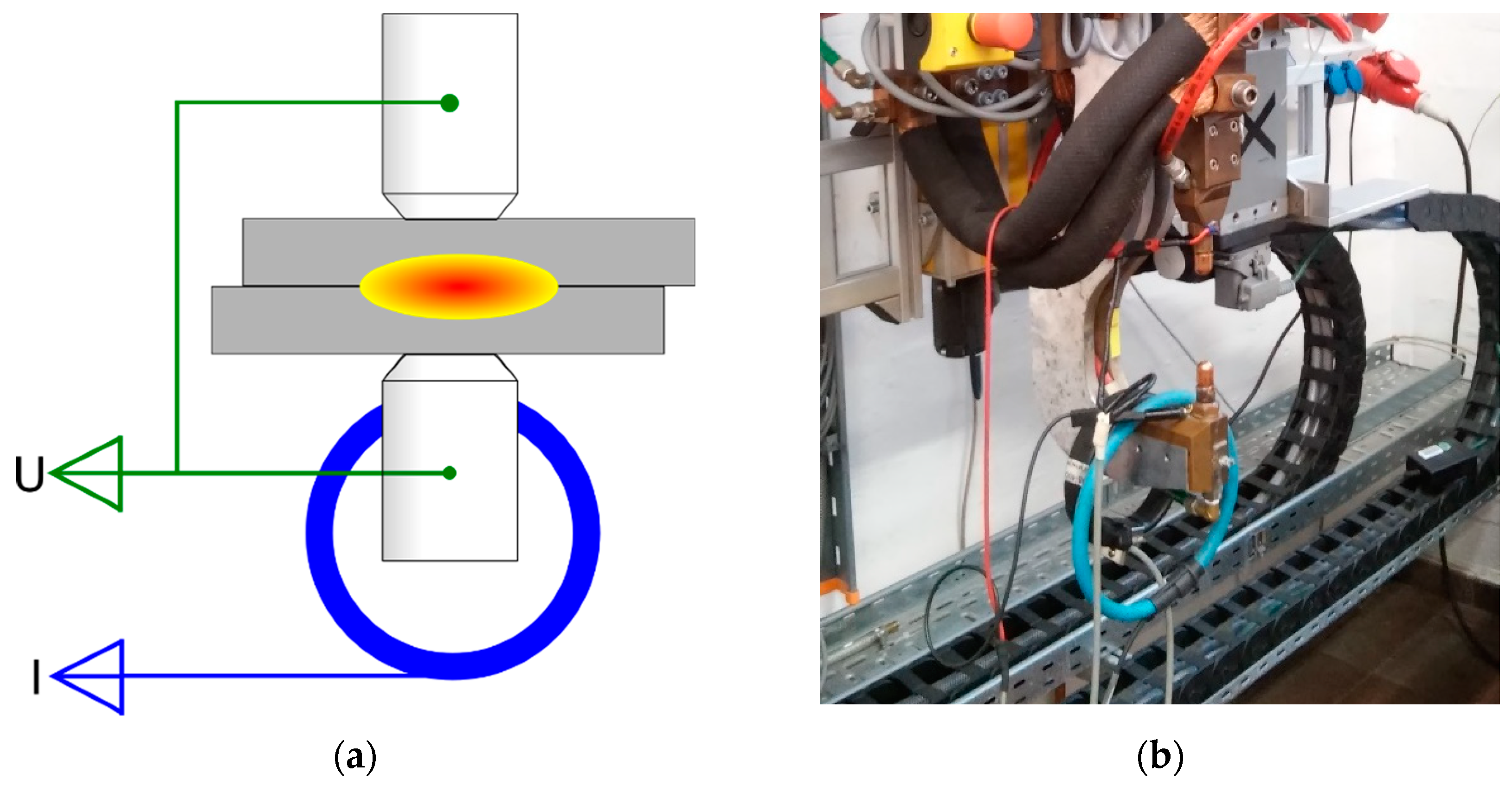
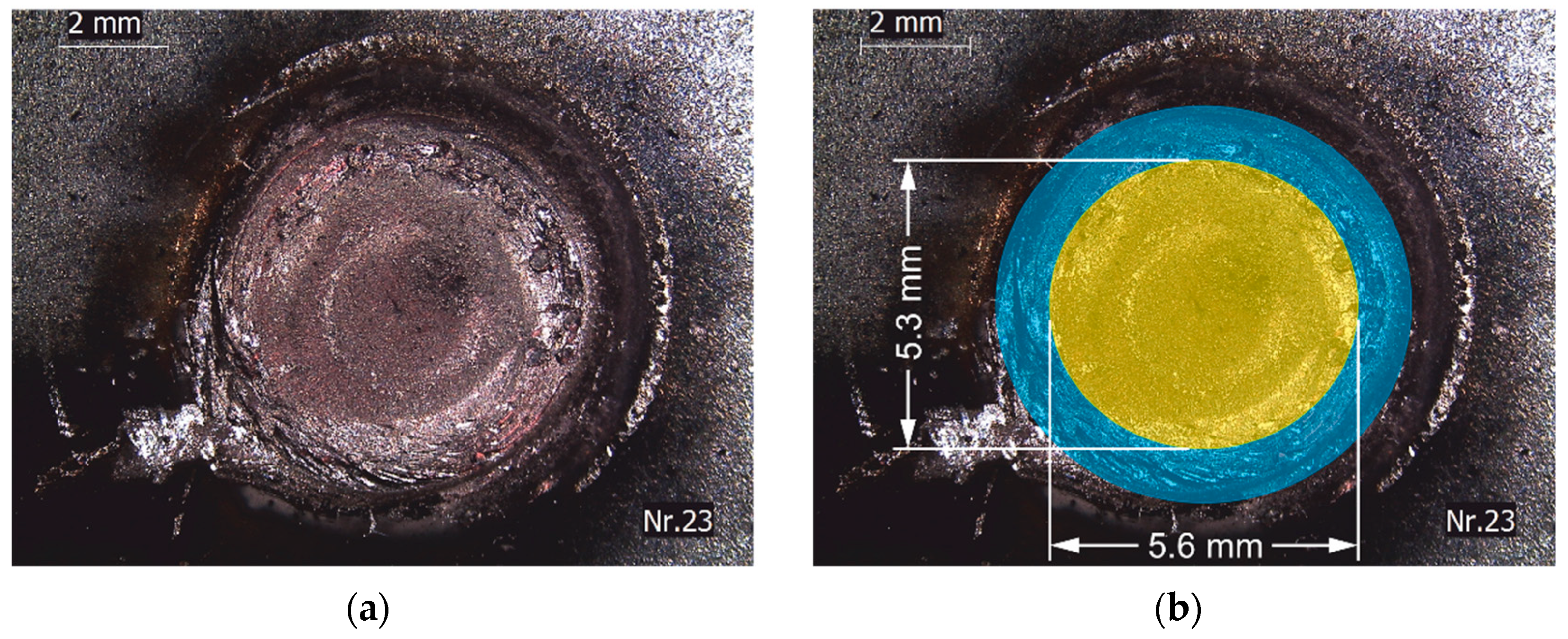
2.1. Experimental Procedure

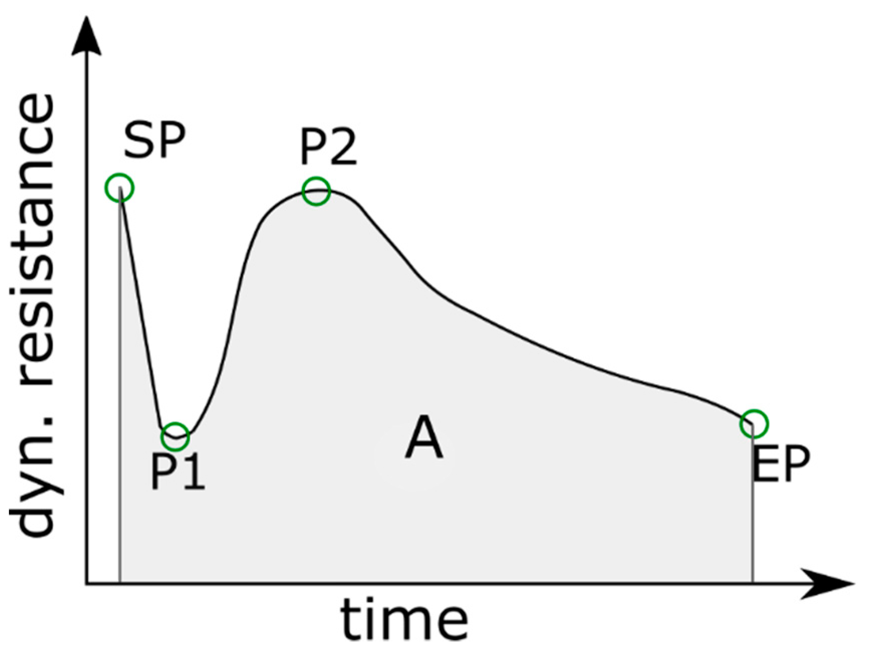
The welding experiments were conducted using a servo-mechanical C-type welding gun (Manufacturer: S.W.A.C, Ödenpullach, Germany), equipped with F1-16-20-8-50-5.5 type electrode caps, according to DIN EN ISO 5821 [30], and a medium frequency inverter power source (Manufacturer: Bosch-Rexroth, Erbach, Germany). The experimental setup is illustrated in Figure 1, it included a Rogowski-coil to measure the current and voltage sensors at the electrodes, to calculate the DR for each weld. The signals were recorded using a SPATZMulti04 Weld Checker, with a maximum sampling rate of 20 kHz and an accuracy of 3% [31], which is adequate for data acquisition in RSW [8].

The welding current range (WCR) for every steel was determined in accordance with the standard Stahl-Eisen-Prüfblatt (SEP) 1220 [32]. Unlike in industry, the electrode force (4.5 kN), the welding time (380 ms), holding time (300 ms), and squeeze time (300 ms) were kept constant during the experiments, only the current was varied. The first weld was done with a current of 3 kA. For the further welds, the current was increased by 200 A per weld, until the first expulsion occurred. Afterwards, the current was reduced by 100 A until no expulsion occurred. The current at which no expulsion occurred was determined as the maximum current of the WCR. In accordance with the standard Stahl-Eisen-Prüfblatt (SEP) 1220 [32], the minimum current of the WCR was the current that created a weld spot that is larger or equal to the minimum spot diameter, which is 4 times the square root of the sheet thickness. A total of 9 test series, with 30 to 50 welds per material, were conducted without repetition. The electrode caps were changed after every test series.

After the welding experiments, destructive testing was conducted to separate the welded sheets and to manually measure the nugget diameter. Afterwards, the recorded process parameters and signals were linked together and saved in a database.

Figure 2a shows an exemplary weld nugget, directly after the torsion testing. In accordance with DVS 2916-1 [33], the fracture surface after a torsion test, can be subdivided into an adhesive zone and the weld nugget. In Figure 2b these areas are marked; the blue ring denotes the adhesive zone, and the yellow area the weld nugget. The weld nugget diameter was determined as the average of vertical and horizontal measurements of the extracted circle.

Table 1. Material overview. Name of materials in accordance with DIN EN 10346:2015 and DIN EN 10152:2017.

No.	Supplier	Name of Material	Sheet Thickness
1	1	HCT 780X +ZM90	1.8
2		HCT 780X +ZE50/50	1.0
3		HCT 780X	1.5
4		HCT 780X +Z100	2.2
5		HCT 780X +Z110	1.5
6		HCT 780X +ZF100	1.5
7		HCT 780X +ZM120	1.5
8	2	HCT 780X +ZM100	1.75
9		HCT 780X +Z140	1.8

lists all the advanced high-strength steels (AHSS) that were used in this work. The sheet thicknesses ranged from 1.0 mm to 2.2 mm. All the materials are of one strength class, but differ in their coating and in the specific material composition, because they were provided by different suppliers.

2.2. Data Analysis

The collected database mainly consists of discrete quantitative data: the applied electrode force, the current the process times, the material names, and their sheet thicknesses. The DR was recorded as time-series data for each spot. All the data were linked through a weld identification number, to assure traceability and to connect the measured diameters to the recorded data.

For pre-processing, a numeric label was assigned to each material, and the data were scaled to reach similar input units. Then, the features of the DR curves were extracted. Two approaches were used in this paper. A manual feature extraction based on physical considerations was performed, and an automated approach using the Python library ‘TSFRESH’ [34] was applied to extract features from the DR curves. Figure 3 shows an exemplary DR curve with a starting point (SP), two peaks (P1 and P2), and an end point (EP). The DR curve can be subdivided into three stages. In the first stage the DR curve drops from the SP to the local minimum P1, due to the current application and the enlargement of the contact surface that forces a decline of the film resistance at the faying surfaces and electrode workpiece interface [29]. The second stage is characterized by a steep rise of the DR until it reaches the local maximum P2, due to the starting of the nugget formation and the accompanying temperature rise. With the initiation of nugget solidification in the third stage, the DR curve sinks from P2 to EP, until the welding process is completed [35]. Furthermore, the area (A) under the curve was also calculated, as it correlates with the heat input, which influences the nugget size.

The feature extraction tool ‘TSFRESH’ calculated a total of 779 time-series features from the DR curve and their statistical significance. Nearly one-third of the features were labelled as statistically significant by ‘TSFRESH’. The five most significant features were taken as input data for the AI algorithm. These features mainly include statistical values that are less descriptive than the manually extracted features from Figure 3 (e.g., the sum of reoccurring data points). However, the global minimum of the curve was also identified as one of the most significant features.

In this work, the extrapolation capabilities of the MLP model was tested. Hence, the available data were mainly subdivided into two datasets. The first dataset included only the data of the materials that were provided by the first supplier, and the second dataset was related to the data of the materials of supplier no. 2. Then, three different models were set up. The first model evaluated only the process parameters, the second model also included the manual extracted features from the DR curve, and the third model was trained with the automatically extracted features. All models were set up as MLP regressors with one hidden layer, using the programming language Python [36] and the library scikit-learn [37].

A MLP regressor is a supervised learning algorithm that learns the following function by training on a dataset [37]:

$$\begin{array}{c}f:R^m\to R^n,\\ f\left(x\right)=w_{11}{x}_1+w_{21}{x}_1+\cdots +w_{km}{x}_m,\end{array}$$

(1)

where x represents the input variables, w is devoted to the weights of the input variables, m is the number of inputs, n represents the number of outputs, and k is the number of neurons of the hidden layer.

The first model has seven input neurons, with one hidden layer and one output layer. The input neurons evaluate the following parameters: current, force, base material, the base thickness, the top material, and the top thickness. The second model includes the following features, which were extracted manually: starting point of the DR curve, end point, area under the curve, first and second peak, and their positions on the timeline. The third model includes the five most significant features from the DR curve, which were extracted using ‘TSFRESH’. The second and the third model have also one hidden layer and one output layer to predict the nugget size. A rectified linear unit function was used for all models as an activation function.

2.3. Evaluation Metric

The deviation between the measured diameters and the predictions was expressed with the relative error of the prediction:

$$\delta =\frac{\left|d_p-d_m\right|}{d_m}\cdot 100\%,$$

(2)

with d_m as the measured nugget diameter and d_p as the prediction.

This metric was calculated for each prediction. Then the calculated values were divided into three groups. The first group contains all predictions with an error of less than 10 %, the second group includes the predictions with an error between 10% and 20%, and the last group contains the predictions with an error larger than 20%. In this work, an error of less than 10% was determined as a good prediction, and a prediction with an error between 10% and 20% was still acceptable; whereas predictions with errors larger than 20% were classified as inaccurate. Then, the predictions in the different groups were counted to calculate the proportion of the groups, in terms of the total number of predictions, and the results were plotted in a bar chart.

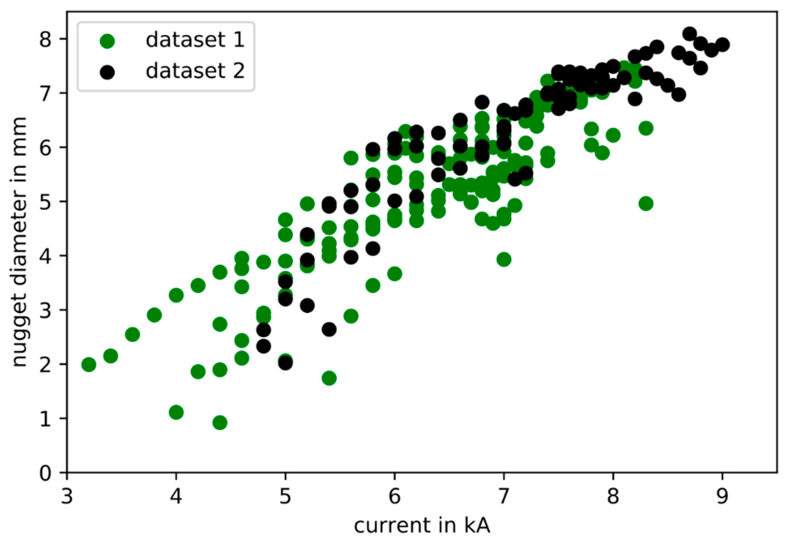
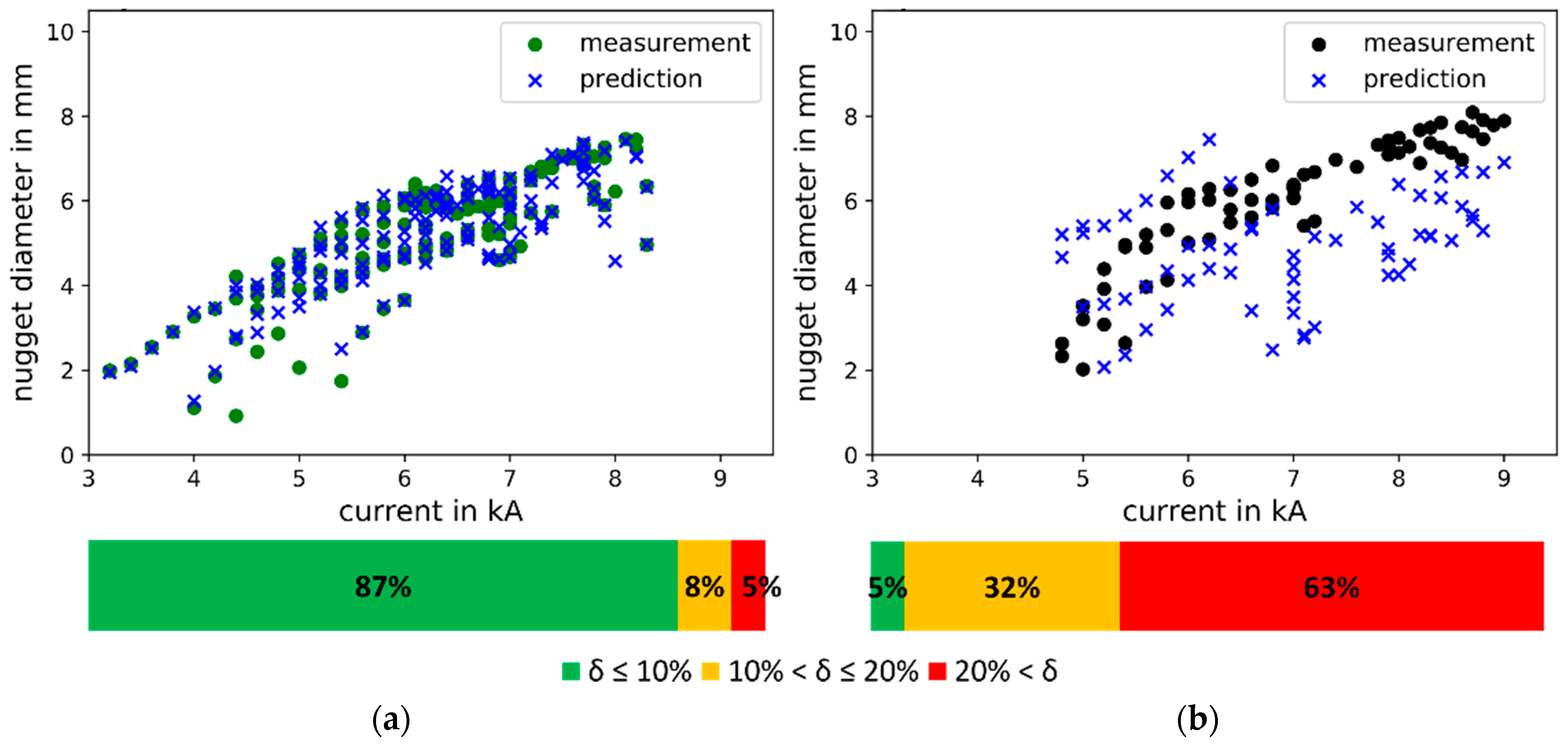
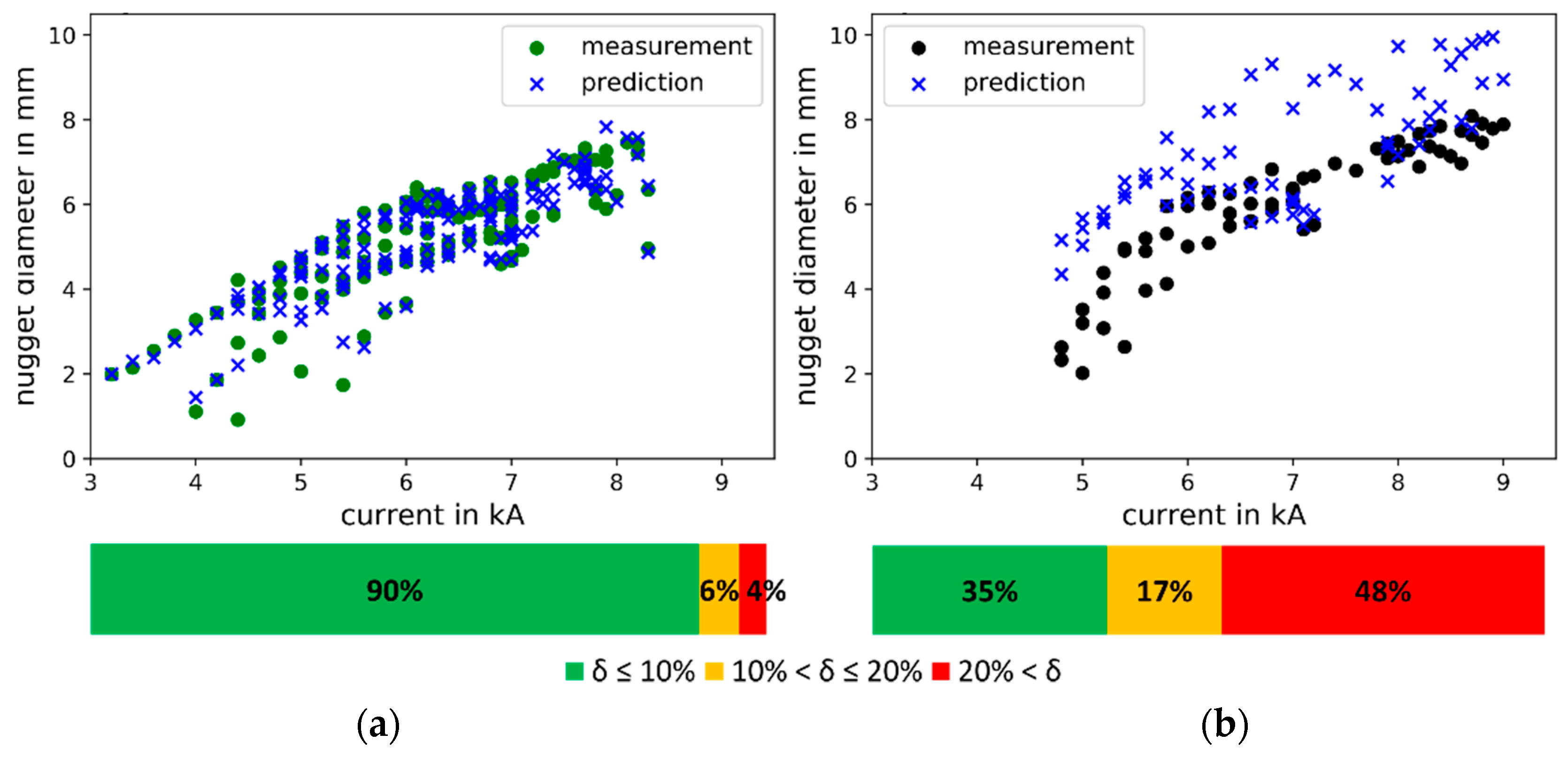
3. Results and Discussion

Figure 4 shows a scatter plot that depicts the nugget diameters over the applied current. It can be seen that the nugget size depends on the applied current. In general, an increase of the current leads to larger nugget diameters. In addition, other parameters (such as electrode force, thickness, and material) have an influence on the nugget formation, which can be seen in the deviations of the nuggets with the same current level. The data are subdivided into two datasets, which differ mainly in the material composition and the coating of the specimens. The first dataset contains only the data related to the specimens that were made out of the materials from supplier 1, and the second dataset represents the specimens that were made out of the materials from supplier 2. Dataset 1 and 2 have some overlaps; however, they differ in the applied process parameters. For example, the weld spots of dataset 1 experienced a current from 3.2 kA to 8.3 kA, whereas the samples of dataset 2 experienced a current between 4.8 kA to 9.0 kA. In dataset 1, three different electrode forces were applied: 3.5 kN, 4.5 kN, and 5.0 kN, whereas in dataset 2 only an electrode force of 4.5 kN was applied. The sheet thickness in dataset 1 ranged from 1.0 mm to 2.2 mm, whereas in dataset 2 only two sheet thicknesses were used: 1.5 mm and 1.8 mm.

The first MLP model was trained only with the process parameters: current, welding time, electrode force, sheet thickness, and material. Figure 5a shows a scatter plot of the measured nugget diameters from dataset 1, and the blue crosses marks the prediction. It can be seen that the algorithm provided a good prediction of the dataset. The bar chart shows that 85% of the predictions had a relative deviation from the measured nugget diameter of less than 10%. Figure 5b shows a scatter plot of the measured nugget diameters from dataset 2, which were not part of the training. Similar to the prior image, the predictions are represented by blue crosses. It is obvious that the model overestimates the nugget diameter and was not able to map the distribution of the nugget diameters correctly. This can also be seen in the bar chart, where 90% of the predictions had a relative deviation from the real nugget diameters of more than 20%.

The second MLP model was trained with the data from dataset 1 and the manual dynamic resistance features. The features were extracted from the curves through the identification of characteristic points: SP, P1, P2, EP, and A. Figure 6a shows a scatter plot of the measured nugget diameters from dataset 1. The algorithm provided a very good prediction of the data set, similarly to the first model. The bar chart shows that 87% were predicted with an acceptable accuracy of less than 10%, and the model was able to map the distribution of the nugget diameters very well. In Figure 6b, the predictions are mostly spatially close to the measurements, with a considerable number of outliers. In comparison to the first model, this model was also able to map the distribution of the nugget diameters of the untrained dataset 2. The bar chart shows that only 5% of the predictions had a relative deviation from the real nugget diameters of less than 10% and 32% had a relative deviation between 10% and 20%. The proportion of predictions with a relative error of more than 20% was still significantly smaller in this model than in the first one.

The third MLP model was implemented with dataset 1 and validated with dataset 2. In addition to the process parameters, the DR curves were also involved in the training. The curves were measured during the experiments and were assigned to each spot. An automated feature extraction tool ‘TSFRESH’ was used to determine the relevant features of the DR curve. Figure 7a shows that the third model achieved the highest accuracy rate in predicting dataset 1. The bar chart shows, that 90% of the predictions had a relative deviation from the measured nugget diameters of less than 10%. From the scatter plot in Figure 7b and the bar chart below it, it is obvious that the third model is the most robust algorithm in this work. The MLP regressor represents the second dataset well, which can be seen in the bar chart. Moreover, 35% of the predictions had a relative deviation from the real nugget diameters of less than 10%, and another 17% had a relative deviation between 10% and 20%. The proportion of predictions with a relative error of more than 20% was significantly smaller in this model than in the first and second models.

The three models were able to predict the dataset 1 well, with an accuracy ranging from 85% to 90%. From this it follows that the structure of the models and the respective input data are sufficient to evaluate the RSW process data and to predict the weld nugget diameter. This was already shown in the literature by Afshari et al. [23]. Similarly to in the work of Boersch et al. [27] and Wan et al. [28], models 2 and 3 achieved higher accuracy rates than model 1, due to the evaluation of the dynamic resistance features.

The models were not able to achieve such high accuracy rates with dataset 2. However, the second and third model were able to yield significantly better results than the first model. Hence, the models which were trained with features from the dynamic resistance curve can be seen as more robust than the first model, which was only trained with process parameters. In contrast to the work of Fabry et al. [26], the second and third models were able to extrapolate to a certain degree. Both models leveraged the characteristic behavior of the dynamic resistance curve [8] to predict the nugget diameter for untrained input parameters. Similar observations were made by Lee et al. [29]. The authors trained their model with calculated features based on wavelet-transformation, and they succeeded in the prediction of data from outside of the trained process parameter space. In terms of predicting a dataset from outside of the parameter space of the training data, the third model performed better than the second one, because it included the most significant features of the dynamic resistance curve.

4. Conclusions

This work aimed to investigate the extrapolation capabilities of an artificial neural network algorithm to predict the nugget diameter of resistance spot welds of advanced high-strength steels. Three multi-layer perceptron models were implemented and trained on the same data set. The models predicted and mapped the training dataset well. Hence, the process parameters and structure of the models were sufficient to represent the RSW process and to predict the nugget diameter. The first model was trained only with process parameters, whereas the second and third model were provided with features from the dynamic resistance curve. This resulted in an increase of the predictive accuracy of both models. Two approaches were used: a manual feature picking, based on the identification of characteristic points on the dynamic resistance curve, and an automated feature extraction tool that calculates a large number of possible features.

The second and third models were able to extrapolate and to predict the nugget diameters from the non-training data set. The latter was more successful in extrapolating, because the most significant features were included. Hence, to ensure a certain level of extrapolation capability and robustness for AI algorithms in RSW, it is essential to involve process signals, such as the dynamic resistance curve, in the training of the AI algorithms and to choose the most significant ones for the training. To realize further improvements of the extrapolation capability, the combination of several models and optimization of the algorithm architecture will be tested in a future work.

References

1. Brauser, S.; Pepke, L.A.; Weber, G.; Rethmeier, M. Deformation behaviour of spot-welded high strength steels for automotive applications. Mater. Sci. Eng. A 2010, 527, 7099–7108. [Google Scholar] [CrossRef]
2. Lei, Z.; Kang, H.; Liu, Y. Finite Element Analysis for Transient Thermal Characteristics of Resistance Spot Welding Process with Three Sheets Assemblies. Procedia Eng. 2011, 16, 622–631. [Google Scholar] [CrossRef] [Green Version]
3. Summerville, C.; Adams, D.; Compston, P.; Doolan, M. Nugget Diameter in Resistance Spot Welding: A Comparison between a Dynamic Resistance Based Approach and Ultrasound C-scan. Procedia Eng. 2017, 183, 257–263. [Google Scholar] [CrossRef]
4. Nielsen, C.V.; Friis, K.S.; Bay, N. Three-Sheet Spot Welding of Advanced High-Strength Steels. Weld. J. 2011, 90, 33–40. [Google Scholar]
5. Williams, N.T.; Parker, J.D. Review of resistance spot welding of steel sheets Part 1 Modelling and control of weld nugget formation. Int. Mater. Rev. 2004, 49, 45–75. [Google Scholar] [CrossRef]
6. Jou, M. Real time monitoring weld quality of resistance spot welding for the fabrication of sheet metal assemblies. J. Mater. Process. Technol. 2003, 132, 102–113. [Google Scholar] [CrossRef]
7. Bosch Rexroth. Adapt and Change: How Adaptive Control of Resistance Welding can Cut Production Costs and Improve Product Quality. Available online: https://m.boschrexroth.com/en/gb/trends-and-topics/adaptive-welding/seoadaptivewelding-2 (accessed on 1 April 2020).
8. Zhang, H.; Senkara, J. Resistance Welding: Fundamentals and Applications, 2nd ed.; CRC Press: Boca Raton, FL, USA, 2012; ISBN 978-1-4398-5371-9. [Google Scholar]
9. Li, Y.; Yan, F.; Luo, Z.; Chao, Y.J.; Ao, S.; Cui, X. Weld Growth Mechanisms and Failure Behavior of Three-Sheet Resistance Spot Welds Made of 5052 Aluminum Alloy. J. Mater. Eng. Perform. 2015, 24, 2546–2555. [Google Scholar] [CrossRef]
10. Ren, J.; Dong, W.; Zhang, Y.; Yu, Z. Failure Analysis of Three-Sheet Stackup Structure Made of Dissimilar High-Strength Steel. J. Mater. Eng. Perform. 2019, 28, 3438–3445. [Google Scholar] [CrossRef]
11. HW-Verlag. Qualitätssicherung und Dokumentation Verbinden. Available online: https://werkstoffzeitschrift.de/qualitaetssicherung-und-dokumentation-verbinden/ (accessed on 13 April 2020).
12. Pereira, A.B.; de Melo, F.J.M.Q. Quality Assessment and Process Management of Welded Joints in Metal Construction—A Review. Metals 2020, 10, 115. [Google Scholar] [CrossRef] [Green Version]
13. Mazumder, J. Design for Metallic Additive Manufacturing Machine with Capability for “Certify as You Build”. Procedia CIRP 2015, 36, 187–192. [Google Scholar] [CrossRef] [Green Version]
14. Holzmond, O.; Li, X. In situ real time defect detection of 3D printed parts. Addit. Manuf. 2017, 17, 135–142. [Google Scholar] [CrossRef]
15. Eggink, D.H.; Groll, M.W. Joining element design and product variety in manufacturing industries. Procedia CIRP 2020, 88, 76–81. [Google Scholar] [CrossRef]
16. Shahin, M.A. State-of-the-art review of some artificial intelligence applications in pile foundations. Geosci. Front. 2016, 7, 33–44. [Google Scholar] [CrossRef] [Green Version]
17. Wang, B.; Hu, S.J.; Sun, L.; Freiheit, T. Intelligent welding system technologies: State-of-the-art review and perspectives. J. Manuf. Syst. 2020, 56, 373–391. [Google Scholar] [CrossRef]
18. Ahmed, F.; Jannat, N.-E.; Schmidt, D.; Kim, K.-Y. Data-driven cyber-physical system framework for connected resistance spot welding weldability certification. Robot. Comput. Integr. Manuf. 2021, 67, 102036. [Google Scholar] [CrossRef]
19. Ashtari, E.; Semere, D.; Melander, A.; Löveborn, D.; Hedegård, J. Knowledge Platform for Resistance Spot Welding. Procedia CIRP 2018, 72, 1166–1171. [Google Scholar] [CrossRef]
20. Panda, B.N.; Babhubalendruni, M.V.A.R.; Biswal, B.B.; Rajput, D.S. Application of Artificial Intelligence Methods to Spot Welding of Commercial Aluminum Sheets (B.S. 1050). In Proceedings of Fourth International Conference on Soft Computing for Problem Solving; Das, K.N., Deep, K., Pant, M., Bansal, J.C., Nagar, A., Eds.; Springer India: New Delhi, India, 2015; pp. 21–32. ISBN 978-81-322-2216-3. [Google Scholar]
21. Ahmed, F.; Kim, K.-Y. Data-driven Weld Nugget Width Prediction with Decision Tree Algorithm. Procedia Manuf. 2017, 10, 1009–1019. [Google Scholar] [CrossRef]
22. Zhou, K.; Yao, P. Overview of recent advances of process analysis and quality control in resistance spot welding. Mech. Syst. Signal Process. 2019, 124, 170–198. [Google Scholar] [CrossRef]
23. Afshari, D.; Sedighi, M.; Reza Karimi, M.; Barsoum, Z. Prediction of the nugget size in resistance spot welding with a combination of a finite-element analysis and an artificial neural network. Mater. Tehnol. 2014, 48, 33–38. [Google Scholar]
24. Arunchai, T.; Sonthipermpoon, K.; Apichayakul, P.; Tamee, K. Resistance Spot Welding Optimization Based on Artificial Neural Network. Int. J. Manuf. Eng. 2014, 2014, 1–6. [Google Scholar] [CrossRef] [Green Version]
25. Martín, Ó.; Ahedo, V.; Santos, J.I.; Tiedra, P.; de Galán, J.M. Quality assessment of resistance spot welding joints of AISI 304 stainless steel based on elastic nets. Mater. Sci. Eng. A 2016, 676, 173–181. [Google Scholar] [CrossRef] [Green Version]
26. Fabry, C.; Pittner, A.; Rethmeier, M. Design of neural network arc sensor for gap width detection in automated narrow gap GMAW. Weld World 2018, 62, 819–830. [Google Scholar] [CrossRef]
27. Boersch, I.; Füssel, U.; Gresch, C.; Großmann, C.; Hoffmann, B. Data mining in resistance spot welding. Int. J. Adv. Manuf. Technol. 2018, 99, 1085–1099. [Google Scholar] [CrossRef]
28. Wan, X.; Wang, Y.; Zhao, D.; Huang, Y.; Yin, Z. Weld quality monitoring research in small scale resistance spot welding by dynamic resistance and neural network. Measurement 2017, 99, 120–127. [Google Scholar] [CrossRef]
29. Lee, J.; Noh, I.; Jeong, S.I.; Lee, Y.; Lee, S.W. Development of Real-time Diagnosis Framework for Angular Misalignment of Robot Spot-welding System Based on Machine Learning. Procedia Manuf. 2020, 48, 1009–1019. [Google Scholar] [CrossRef]
30. DIN EN ISO 5821:2010-04. Resistance Welding—Spot Welding Electrode Caps (ISO 5821:2009). Available online: https://www.beuth.de/en/standard/din-en-iso-5821/123603505 (accessed on 1 October 2021).
31. Matuschek Meßtechnik GmbH. SpatzMulti04 Weld Checker & Monitor for RSW. Available online: https://www.matuschek.de/weld-monitoring/multi04-weld-monitor.htm (accessed on 1 June 2021).
32. SEP-1220-2:2011-08. Prüf- und Dokumentationsrichtlinie für die Fügeeignung von Feinblechen aus Stahl: Teil 2: Widerstandspunktschweißen. Available online: https://www.beuth.de/en/technical-rule/sep-1220-2/153435334 (accessed on 15 September 2021).
33. DVS 2916-1:2014-03. Testing of Resistance Welded Joints—Destructive Testing, Quasi Static. Available online: https://www.beuth.de/en/technical-rule/dvs-2916-1/200030552 (accessed on 5 June 2021).
34. Christ, M.; Braun, N.; Neuffer, J.; Kempa-Liehr, A.W. Time Series FeatuRe Extraction on basis of Scalable Hypothesis tests (tsfresh—A Python package). Neurocomputing 2018, 307, 72–77. [Google Scholar] [CrossRef]
35. Wang, S.C.; Wei, P.S. Modeling Dynamic Electrical Resistance During Resistance Spot Welding. J. Heat Transf. 2001, 123, 576–585. [Google Scholar] [CrossRef]
36. Van Rossum, G. The Python Language Reference, Release 3.0.1 [Repr.]; Python Software Foundation: Hampton, NH, USA; SoHo Books: Redwood City, CA, USA, 2010; ISBN 978-1-4414-1269-0. [Google Scholar]
37. Pedregosa, F.; Varoquaux, G.; Gramfort, A.; Michel, V.; Thirion, B.; Grisel, O.; Blondel, M.; Prettenhofer, P.; Weiss, R.; Dubourg, V.; et al. Scikit-learn: Machine Learning in Python. J. Mach. Learn. Res. 2011, 12, 2825–2830. [Google Scholar]
Figure 1. Experimental setup. (a) Schematic of the welding setup; (b) footage of the welding gun with a Rogowski coil and voltage sensors.
Metals 11 01874 g001
Figure 2. Exemplary specimen after torsion testing: (a) weld nugget after torsion testing; (b) adhesive zone is represented by the blue ring, and the yellow circle marks the weld nugget.
Metals 11 01874 g002
Figure 3. Typical DR curve for steel. The following features are marked: starting point (SP), peak no. 1 (P1), peak no. 2 (P2), end point (EP), and area (A) under the curve.
Metals 11 01874 g003
Figure 4. Data overview. Green spots mark the measured diameters from supplier 1, and black spots from supplier 2.
Metals 11 01874 g004
Figure 5. Predictive performance of the first model. Only process parameters were used as input for training: (a) scatter plot of the measured and predicted nugget diameters from dataset 1; (b) scatter plot of the measured and predicted nugget diameters from dataset 2. The bar charts show the predictive accuracy based on the prescribed deviation.
Metals 11 01874 g005
Figure 6. Predictive performance of the second model. The training included manually extracted dynamic resistance features: (a) scatter plot of the measured and predicted nugget diameters from dataset 1; (b) scatter plot of the measured and predicted nugget diameters from dataset 2. The bar charts show the predictive accuracy based on the prescribed deviation.
Metals 11 01874 g006
Figure 7. Predictive performance of the third model. The training included the dynamic resistance features extracted by ‘TSFRESH’: (a) scatter plot of the measured and predicted nugget diameters from dataset 1; (b) scatter plot of the measured and predicted nugget diameters from dataset 2. The bar charts show the predictive accuracy based on the prescribed deviation.
Metals 11 01874 g007