Hot Deformation Behavior of a Beta Metastable TMZF Alloy: Microstructural and Constitutive Phenomenological Analysis

Abstract

A metastable beta TMZF alloy was tested by isothermal compression under different conditions of deformation temperature (923 to 1173 K), strain rate (0.172, 1.72, and 17.2 s⁻¹), and a constant strain of 0.8. Stress–strain curves, constitutive constants calculations, and microstructural analysis were performed to understand the alloy’s hot working behavior in regards to the softening and hardening mechanisms operating during deformation. The primary softening mechanism was dynamic recovery, promoting dynamic recrystallization delay during deformation at higher temperatures and low strain rates. Mechanical twinning was an essential deformation mechanism of this alloy, being observed on a nanometric scale. Spinodal decomposition evidence was found to occur during hot deformation. Different models of phenomenological constitutive equations were tested to verify the effectiveness of flow stress prediction. The stress exponent $n$, derived from the strain-compensated Arrhenius-type constitutive model, presented values that point to the occurrence of internal stress at the beginning of the deformation, related to complex interactions of dislocations and dispersed phases.

1. Introduction

TMZF is a metastable beta titanium alloy specially developed for medical applications. Its main characteristics are the low elastic modulus associated with its cubic phase [1] and a chemical composition that avoids elements that have been identified as cytotoxic [2,3]. The elastic modulus varies from 70 to 90 GPa, reducing stress shielding phenomena [1]. Besides the low modulus, beta alloys have relatively good workability due to their low beta transus temperature compared to the conventional α + β titanium alloys [4].

The flow stress behavior during the hot deformation process can be highly complex to predict since hardening and softening phenomena are influenced by numerous factors, such as the accumulated strain, strain rate, and temperature under which thermomechanical processing is performed. The combination of processing parameters leading to metallurgical phenomena and the consequent microstructure modifications, along with the deformation evolution, directly impact the flow behavior. Therefore, it is paramount to model or design thermomechanical processes to understand how the relationship between flow stress and strain interacts in metallic materials and alloys and the kinetics of metallurgical transformations to predict the final microstructure.

In metal forming simulation software programs based on finite element method (FEM) calculations, it is possible to write subroutines to insert different models of constitutional equations so that the relationships between the factors mentioned above can be calculated. Therefore, it is possible to simulate the stresses and strains occurring due to loads, restrictions, and additional boundary conditions using such software programs. Hence, an ideal plastic model should accurately describe the material’s properties, i.e., the dependence of the stress behavior on all process variables, including their initial properties (deformation history, grain size, etc.). However, the complete description of all phenomena that may occur is tough to obtain. In this way, changes in some of the parameters of the equations are carried out in the existing constitutive models to adapt the existent equations to different metallurgical behaviors [5].

Constitutive equations are mainly divided into phenomenological constitutive, physical constitutional, and artificial neural network models. Phenomenological constitutive models define stress based on a set of empirical observations and consist of some mathematical functions. However, phenomenological models are not physically based, rather, they only adjust the proposed models with a basis on experimental results. Although they are not based on physical phenomena, these models have a positive quality of not requiring extensive empirical data to determine the material’s constants for the equations and they are easily calibrated. The disadvantage of using this type of modeling is that, due to their empirical characteristics, their use is generally limited to specific application fields, as they cover only limited ranges of strain rates and temperatures, exhibiting reduced flexibility. Several phenomenological models were developed to describe the behavior of metals or alloys during plastic deformation. The main similarity between such models is that they can be expressed as a function of the temperature, strain rate, and accumulated deformation to consider the effects of these process parameters on the flow stress [6].

Three models and their variations with few modifications will be discussed in the present work to evaluate their effectiveness in predicting the stress flow behavior of a beta metastable TMZF alloy. Specifically, we analyzed the modified models of Johnson–Cook and Zerilli–Armstrong, and the strain-compensated Arrhenius-type equation.

Due to the high stacking fault energy of beta titanium alloys, they undergo continuous dynamic recrystallization (CDRX) when deformed under high temperatures. CDRX results from the high efficiency of the dynamic recovering process. Therefore, new grains gradually transform subgrains into new grains from the highly deformed original grains. During the deformation process, the dislocations are progressively accumulated in low-angle boundaries (subgrains), following which the misorientation of these boundaries increases and changes to high-angle boundaries, forming new grains. This process is accompanied by a strong crystallographic texture (at large strains) and grain boundary migration [7]. CDRX has also been considered a particular type of dynamic recrystallization, usually related to neck-lacing recrystallization [4]. The nucleation of new recrystallized grains occurs by serration and bulging of grain boundaries [8].

In addition to the fact that the cubic phase may undergo different softening mechanisms in distinct processing conditions, it is known that these alloys are likely to facilitate the formation of the metastable omega phase due to the high amount of beta-stabilizing elements [9]. Such beta-stabilizing elements interact with the sliding that occurs as a result of the dislocations, leading to the hardening of the alloy and changes in the activation energy for the occurrence of dynamic recrystallization.

It has been reported that the omega phase can form in two ways, the first is due to fast cooling from high temperatures, giving rise to the athermic omega phase. The second is due to aging at intermediate temperatures, called the thermal omega phase [10]. Its formation has been related to another coherent phase resulting from a spinodal reaction of the beta phase, giving rise to a solute-rich phase and a poor one, with the latter being reported as a precursor to the omega phase formation [6,7]. Although the appearance of the omega phase has been communicated for the above phenomena, it is still unclear how the omega phase precipitation is influenced by the hot deformation process and the spinodal decomposition.

It has also been discussed that the omega phase can precipitate in a manner induced by deformation in beta metastable alloys during cold deformation [11], i.e., an increase in the volumetric fraction of the omega phase may occur during deformation. However, no studies were found about quantifying the omega phase in beta metastable alloys under hot deformation.

In addition, a close correlation between deformation by twinning and reverse transformation of the omega phase has been reported. A thin layer of omega phase can be found along the twin contours of {332}_β or {112}_β in Ti-15Mo-5Zr and Ti-Nb alloys [12]. This contour phase appears in alloys that already presented an athermal omega phase before deformation. Wu et al. [13] proposed that {112} <111> twins are nucleated inside omega phase particles and that the occurrence of twinning is dependent on the reverse transformation of ω → β, with this transformation being the driving force for twinning and the instability of the metastable omega phase precursor. In this way, the occurrence of twinning may reduce the fraction of the omega phase.

Based on the facts mentioned above, it is challenging to correlate the flow stress data obtained on these controlled tests to the resulting microstructure, softening, and hardening phenomena. This work aimed to contribute to the general understanding of metastable beta alloys’ behavior under hot deformation conditions.

2. Materials and Methods

2.1. Material Characterization

The TMZF alloy used in the present work was received in ingot form and produced by Ercata GmbH according to ASTM F1813 standard. The composition of the as-cast alloy, obtained by inductively coupled plasma optical emission spectrometry (Varian ICP-OES Vista AX, Palo Alto, CA, USA) and by a LECO ONH-836 analyzer (LECO, Geleen, The Netherlands), was determined to be ~86.5 wt% Ti, 11 wt% Mo, 2.3 wt% Fe, 0.155 wt% O, 0.0213 wt% N, and 0.00223 wt% H, per the alloy specification. After cutting, the ingot was hot-rotary-swaged at 1173 K. Round bars 16 mm in diameter were obtained to be further machined into cylindrical specimens.

The rotary-swaged bars were subjected to a solution heat treatment at 1273 K for 0.5 h followed by water quenching to promote only the presence of the beta phase in the initial condition of the tests.

For microstructure observations (initial condition and deformed samples), conventional metallographic procedures were used, followed by polishing in a solution of 3% HF, 3% HNO₃, and 94% alumina 0.3 µm in suspension. The images were acquired by an AxioCam ERc 5s camera coupled to a LEITZ Laborlux 12 ME optical microscope (LEITZ, Oberkochen, Germany). A Tecnai G² F20 transmission electron microscope (TEM, FEI, Eindhoven, The Netherlands) was utilized for omega phase investigation with an operating voltage of 200 kV.

The deformed specimens were sectioned with their cylinder axis parallel to the compression axis to be analyzed by OM. For high-contrast scanning electron microscopy (SEM- FEI Inspect S 50) using a back-scattered electron detector (BSED), (FEI, Eindhoven, The Netherlands), the samples were polished on a Buhler VibroMet^TM2 vibratory polisher with 0.05 μm colloidal silica suspension using a weight upon the specimens and then analyzed on an SEM FEI Inspect S50. Twinning was investigated by phase mapping and crystallographic orientation performed in a TEM FEI TECNAI G2 S’TWIN with LaB₆ filament equipped with a Nanomegas A-Star system.

X-ray diffraction analyses were performed on a Bruker D8 Advance ECO machine at 298 K, scanning from 5 to 90°, with 0.02° steps and an integration time of 0.5 s in a Cu tube -kα (0.15406 nm) using Bragg–Brentano geometry.

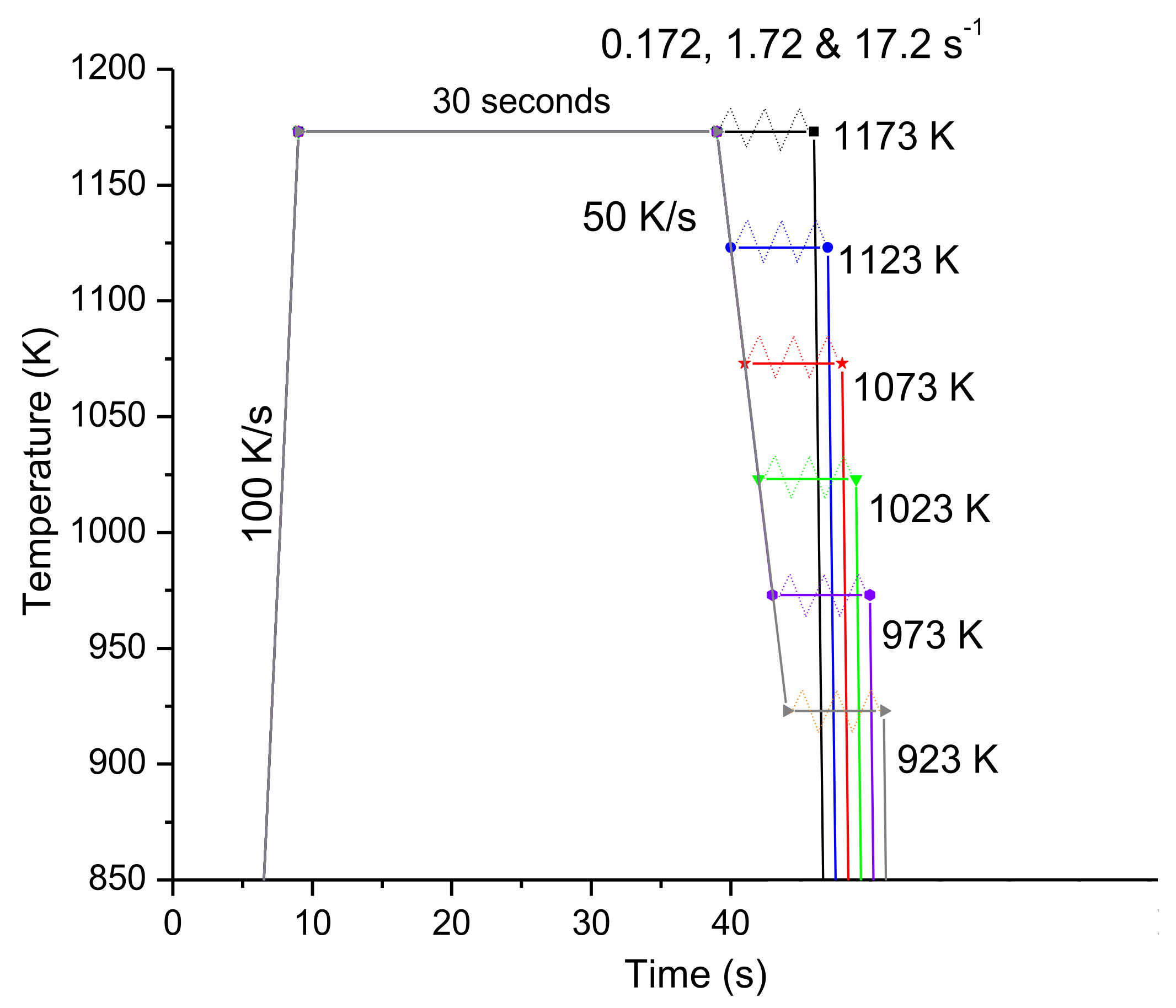
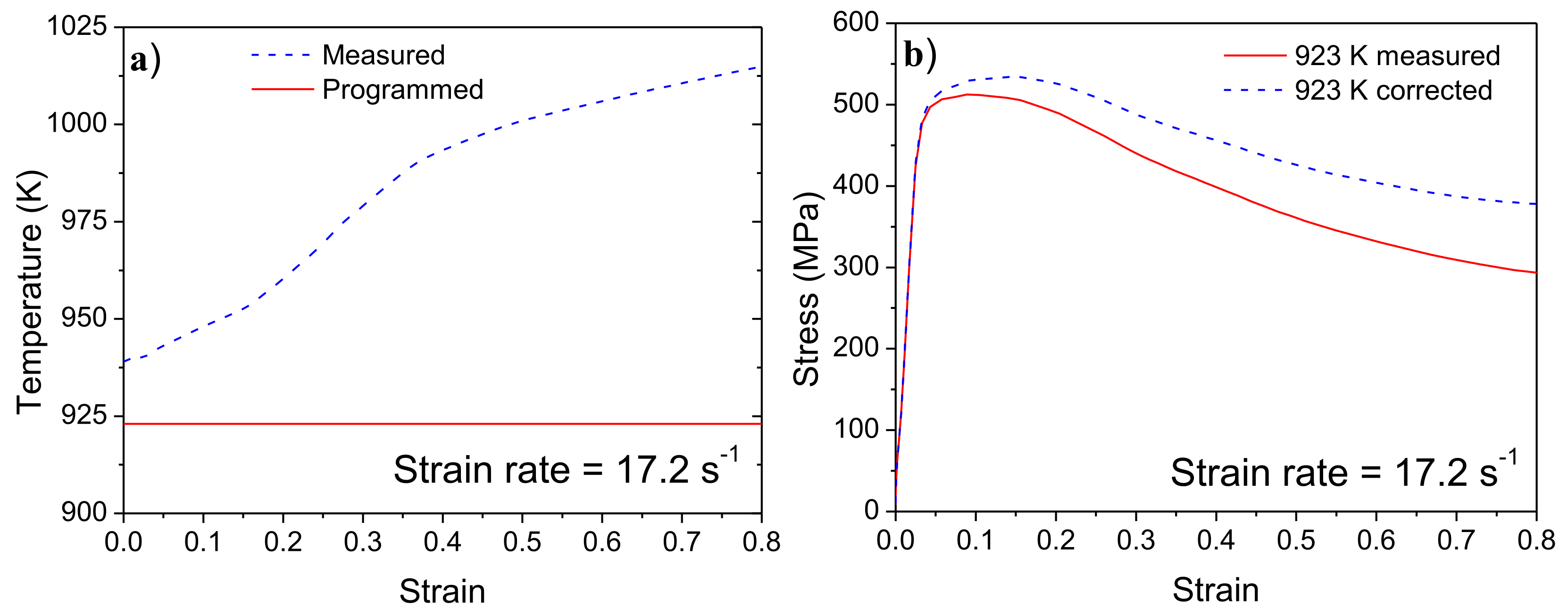
2.2. Compression Tests

Cylindrical specimens 6 mm in diameter and 9 mm in height were machined from swaged and heat-treated bars by wire electrical discharge machining (EDM, Suprasonic Eletrônica LTDa, Varzea Paulista, SP, Brazil). The samples were deformed isothermally under compression at three strain rates: 0.172, 1.72, and 17.2 s⁻¹, at six temperatures starting from 923 K up to 1173 K, with incremental steps of 50 K, providing a total of 18 different parameter combinations. The steps and parameters used in the tests are described in the schematic illustration shown in Figure 1.

The hot compression tests were carried out on a conventional thermo-mechanical simulator—Gleeble^® 3800 (Dynamic Systems Inc., Poestenkill, NY, USA). The facility that we used is part of the National Center for Research in Energy and Materials (CNPEM, Campinas-SP, Brazil). All the specimens were pre-heated 1173 K at a heating rate of 100 K·s⁻¹, held for 30 s to eliminate thermal gradients, and then cooled at 50 K·s⁻¹ to the final testing temperature. All deformations were applied at a constant strain rate up to a true strain of about 0.8 and then were immediately cooled to room temperature. Two S-type thermocouple wires were welded before the test on two spots at the mid-span of each compression sample to provide better signals for accurate feedback control of the proposed temperatures. For the sake of reducing friction at the specimen and die interface, a 0.127 mm thick niobium foil disk with a diameter of 15.0 mm and a high-temperature anti-seize lubricant composed of nickel and graphite was inserted between the specimen ends and anvils.

The characteristic compression barreling effect was considered. The data of true stress were firstly corrected by the methodology described in reference [14] to eliminate this error effect on measured stresses. The second source of stress deviation was the adiabatic heating that occurred in the material and, eventually, raised the samples’ temperature, since the Gleeble heating system (induction heating) was not efficient enough to stabilize the temperature and, consequently, differences between the target and the instantaneous temperature (measured by a thermocouple) were verified. This temperature difference (ΔT = T_{instantaneous} − T_target) was used to correct the flow stress curves according to the following expression [15]:

$$∆T=\frac{0.9 {\beta }^{\prime } {{\displaystyle \int }}_0^{\epsilon }\sigma d\epsilon }{\rho Cp}$$

(1)

where ΔT is the temperature increase caused by the adiabatic heating, $\rho$ is the alloy’s density, C_p is the heat capacity, and β′ is the strain-dependent factor, which is assumed to vary between 0.2 and 0.8 for strain rates of 0.001 to 1 s⁻¹. σ is the true stress, ε is the true strain, and 0.9 represents the amount of mechanical work converted into heat. From Equation (1), the equivalent stress was estimated using $\rho$ = 4.98 g/cm³ and C_p = 500 J/K·kg.

2.3. Constitutive Equation Constant Determination

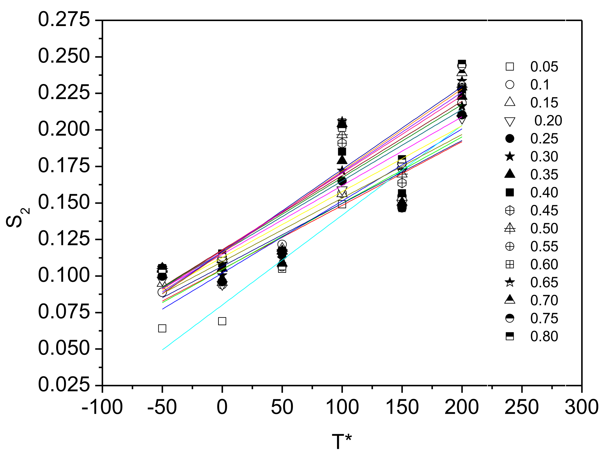
2.3.1. Strain-Compensated Arrhenius-Type Equation

A hyperbolic sine Arrhenius-type relationship was used to proceed with the constitutive constant’s determination, such as the apparent activation energy and stress exponents. Therefore, to consider the role of the total deformation, these constants were determined in true strain steps of 0.05, and a polynomial function was fitted to describe the evolution behavior of such constants. The Arrhenius-type model describes the constitutive equation of the dependence between flow stress, temperature, and strain rate and may also be represented by the Zener–Hollomon parameter in an exponent-type equation. Equations (2)–(4) describe the above mentioned equations [16,17]:

$$\dot{\epsilon }=AF\left(\sigma \right)\exp \left[-\mathrm{Q}/\left(\mathrm{RT}\right)\right]$$

(2)

$$F\left(\sigma \right)=\{\begin{array}{c}{\sigma }^{n^{\prime }} \alpha \sigma <0.8\\ \exp \left(\beta \sigma \right) \alpha \sigma >1.2\\ {\left[sinh\left(\alpha \sigma \right)\right]}^n for all \sigma \end{array}$$

(3)

$$Z=\dot{\epsilon }\exp \left[Q/\left(RT\right)\right]$$

(4)

where $\dot{\mathit{\epsilon }}$ is the strain rate (s⁻¹); $\mathit{\sigma }$ is the stress (MPa); $\mathit{A}$, $\mathit{n}$′, $\mathit{n}$, $\mathit{\alpha }$, and $\mathit{\beta }$ are material constants; $\mathit{Q}$ is the activation energy for hot deformation (J.mol⁻¹); $\mathit{T}$ is the absolute temperature (K); and R is the universal gas constant (8.314 J/(mol.K)). $\mathit{\alpha }$, $\mathit{\beta }$, and $\mathit{n}$′ are related by $\mathit{\alpha }=\mathit{\beta }$⁄$\mathit{n}$′. The material constant $\mathit{n}$′ is called the stress exponent ($\mathit{n}$′ = 1/$\mathit{m}$, $\mathit{m}$ is the strain rate sensitivity).

The first term of Equation (4), ${\mathit{\sigma }}^{{\mathit{n}}^{\prime }}$, represents power law, adequately describing stress behavior at low stresses. At the same time, $\mathbf{exp}\left(\mathit{\beta }\mathit{\sigma }\right)$ refers to the exponential law, which describes the deformation at higher stresses. The power law is not valid at higher stresses as $\mathit{n}$′ varies with the strain rate. The exponential law breaks down at high temperatures below the strain rate of 1 s⁻¹ [16,18,19].

The hyperbolic sine function works better on a wide range of stresses, described using Equations (3) and (4). The constant $\mathit{\alpha }$ is called the stress multiplier, and, as stated above, it is obtained from the relation $\mathit{\alpha }=\mathit{\beta }/{\mathit{n}}^{\prime }$. This constant is used in the hyperbolic sine equation. It has the function of bringing $\mathit{\alpha }\mathit{\sigma }$ to a correct range, making the plots of $\mathit{l}\mathit{n}\dot{\mathit{\epsilon }}$ against $\mathit{l}\mathit{n}\left[\mathit{s}\mathit{i}\mathit{n}\mathit{h}\left(\mathit{\alpha }\mathit{\sigma }\right)\right]$ (at constant temperature) linear and parallel [6]. The combination of Equations (2) and (4) takes the form of the following flow stress relation:

$$\sigma =\frac{1}{\alpha }\left\{{\left(\frac{Z}{A}\right)}^{\raisebox{1ex}{$1$}\!\left/ \!\raisebox{-1ex}{$n$}\right.}+{\left[{\left(\frac{Z}{A}\right)}^{\raisebox{1ex}{$2$}\!\left/ \!\raisebox{-1ex}{$n$}\right.}+1\right]}^{\raisebox{1ex}{$1$}\!\left/ \!\raisebox{-1ex}{$2$}\right.}\right\}$$

(5)

In most of the works using the Arrhenius-type (sine hyperbolic relation) equation, the impact of the strain on the flow stress is not considered. In this way, the material constants are calculated at peak stress. However, in some applications, as in thermomechanical processing simulations, it is essential to understand how the material behaves from the beginning of deformation and after the deformation is accumulated since the stress–strain curves are affected by strain hardening, dynamic softening, etc. Strains in the range of 0.05 to 0.8 in steps of 0.05 were used to define the relationship between the materials’ constants and true strain considering the compensation of strain and to obtain an accurate prediction of the flow stress. Thereby, a polynomial relation was fitted for each calculated constant as a function of the true strain. The polynomial Equation (6) relates material constants to true strain.

$$\left\{\begin{array}{c}\alpha =b\left(\epsilon \right)=B_0+B_1\epsilon +B_2{\epsilon }^2+B_3{\epsilon }^3+B_4{\epsilon }^4+B_5{\epsilon }^5+B_6{\epsilon }^6+B_7{\epsilon }^7+B_8{\epsilon }^8+B_9{\epsilon }^9 \\ \ln \left(A\right)=c\left(\epsilon \right)=C_0+C_1\epsilon +C_2{\epsilon }^2+C_3{\epsilon }^3+C_4{\epsilon }^4+C_5{\epsilon }^5+C_6{\epsilon }^6+C_7{\epsilon }^7+C_8{\epsilon }^8+C_9{\epsilon }^9\\ Q=d\left(\epsilon \right)=D_0+D_1\epsilon +D_2{\epsilon }^2+D_3{\epsilon }^3+D_4{\epsilon }^4+D_5{\epsilon }^5+D_6{\epsilon }^6+D_7{\epsilon }^7+D_8{\epsilon }^8+D_9{\epsilon }^9\\ n=e\left(\epsilon \right)=E_0+E_1\epsilon +E_2{\epsilon }^2+E_3{\epsilon }^3+E_4{\epsilon }^4+E_5{\epsilon }^5+E_6{\epsilon }^6+E_7{\epsilon }^7+E_8{\epsilon }^8+E_9{\epsilon }^9\end{array}\right.$$

(6)

The resulting improved Arrhenius-type equation with the polynomial functions of Equation (6) put into the Equation (5) becomes:

$$\{\begin{array}{c}\sigma =\frac{1}{b\left(\epsilon \right)}ln\left\{{\left(\frac{Z_{d\left(\epsilon \right)}}{exp\left[c\left(\epsilon \right)\right]}\right)}^{\frac{1}{e\left(\epsilon \right)}}+{\left[{\left(\frac{Z_{d\left(\epsilon \right)}}{exp\left[c\left(\epsilon \right)\right]}\right)}^{\frac{2}{e\left(\epsilon \right)}}+1\right]}^{\frac{1}{2}}\right\}\\ Z=\dot{\epsilon }exp\left[\frac{d\left(\epsilon \right)}{RT}\right]\end{array}$$

(7)

2.3.2. Modified Johnson–Cook Model

The Johnson–Cook is the most well-known phenomenological model that relates the flow stress to strain, strain rate, and temperature, being primarily used to describe the flow behavior of several materials in different strain rate and temperature ranges. The advantage of this model is its relative simplicity and the large number of constant values available in the literature. The original Johnson–Cook model is described in Equation (8) [19]:

$$\sigma =\left(A+B{\epsilon }^n\right)\left(1+Cln{\dot{\epsilon }}^{*}\right)\left(1-T^{*m}\right)$$

(8)

where $\sigma$ is the equivalent stress, ε is the equivalent plastic strain, $A$ is the yield stress of the material under different deformation conditions in MPa, $B$ is the strain hardening constant (MPa), $n$ is the strain hardening coefficient, $C$ is the strain rate hardening coefficient, and $m$ the thermal softening exponent. ${\dot{\epsilon }}^{*}=\frac{\dot{\epsilon }}{{\dot{\epsilon }}_{ref}}$ is a dimensionless strain rate relation, where $\dot{\epsilon }$ is the strain rate and ${\dot{\epsilon }}_0$ is the reference strain rate. $T^{*}$ is the homologous temperature, expressed by $T^{*}=(T-T_{ref}/\left(T_m-T_{ref}\right)$, where $T_{ref}$ is the reference temperature, $T_m$ is the melting temperature, and $T$ is the current temperature.

The Johnson–Cook model (Equation (8)) considers the effect of work hardening, the strain rate hardening effect, and temperature on the flow stress as three independent phenomena, wherefore it regards that these effects can be isolated from each other. In addition, the strain softening effect is ignored in the J-C model. The original model is suitable for materials where flow stress is relatively dependent on strain rate and temperature. The J-C model is often implemented in finite element simulation because it is simple, needs few experiments, and has low fitting complexity. However, the assumption of independence of the above phenomena remarkably diminishes the prediction precision. It fails to satisfy the engineering calculation demands. Taking into account all those issues, Lin et al. have proposed a modified J-C model to consider the interaction between the parameters mentioned above, as follows [6]:

$$\sigma =\left(A_1+B_1\epsilon +B_2{\epsilon }^2\right)\left(1+C_{1}ln{\dot{\epsilon }}^{*}\right)exp\left[\left({\lambda }_1+{\lambda }_2\ln {\dot{\epsilon }}^{*}\right)\left(T-T_{ref}\right)\right]$$

(9)

where $A_1$, $B_1$, $B_2$, $C_1$, ${\lambda }_1$e, and ${\lambda }_2$ are material constants and $\sigma$, $\epsilon$, ${\dot{\epsilon }}^{*}$, $T,$ and $T_{ref}$ have the same meaning as the original model.

The present work’s first item of Equation (9) was modified to better describe the flow stress behavior concerning the applied strain. A third-degree polynomial form was utilized, since this modification better described the TMZF flow stress, as detailed in Equation (10).

$$\sigma =\left(A_1+B_1\epsilon +B_2{\epsilon }^2+B_3{\epsilon }^3 \right)\left(1+C_{1}ln{\dot{\epsilon }}^{*}\right)exp\left[\left({\lambda }_1+{\lambda }_2\ln {\dot{\epsilon }}^{*}\right)\left(T-T_{ref}\right)\right]$$

(10)

In this model, the stress is computed at each amount of deformation by the first polynomial term of Equation (10), which allows dynamic hardening and softening phenomena to be considered, as the strain-compensated Arrhenius model, previously cited, does.

2.3.3. Modified Zerilli–Armstrong Model

The Zerilli–Armstrong (ZA) model was initially developed based on dislocation movement mechanisms, composed of two terms, one influenced by thermic factors and the other by an athermic factor. Again, researchers modified the initial proposed model to consider the coupling effect of $T$, $\epsilon$, and $\dot{\epsilon }$ on the flow stress behavior. Samarantay et al. [16] proposed a modification to the ZA model to better describe the behavior of titanium-modified austenitic stainless steel. This model has been used to model titanium alloys and is described in Equation (11):

$$\sigma =\left(C_1+C_2{\epsilon }^n\right)\exp \left\{-\left(C_3+C_4\epsilon \right)T^{*}+\left(C_5+C_6{T}^{*}\right)ln{\dot{\epsilon }}^{*}\right\}$$

(11)

in this equation, $T^{*}=\left(T-T_{ref}\right)$, where $T$ is the current test temperature; $T_{ref}$ is the reference temperature; ${\dot{\epsilon }}^{*}=\frac{\dot{\epsilon }}{{\dot{\epsilon }}_{ref}}$ as in the modified JC model; and $C_1$, $C_2$, $C_3$, $C_4$, $C_5$, $C_6,$ and $n$ are graphically determined material constants. This model considers the isotropic hardening, thermic softening, strain rate hardening, and the coupling effect of strain—temperature and strain-rate—temperature on the flow behavior.

In the present work, the first term of Equation (11) was also altered since the power law does not represent the work hardening of the alloy adequately. Therefore, a third-order polynomial equation was fitted from the reference data (strain rate and temperature references), and its constants were determined. The final modified ZA model used in this work is described in Equation (12).

$$\sigma =\left(A_1+B_1\epsilon +B_2{\epsilon }^2+B_3{\epsilon }^3\right)\exp \left\{-\left(C_3+C_4\epsilon \right)T^{*}+\left(C_5+C_6{T}^{*}\right)ln{\dot{\epsilon }}^{*}\right\}$$

(12)

2.4. Predictability Comparison

The effectiveness of the constitutive models in performing the stress values prediction was evaluated by the adjusted R-squared coefficient (R²), root mean square error (RMSE), and average absolute relative error (AARE), which are described in Equations (13)–(15) [20].

$$R^2=1-\frac{{{\displaystyle \sum }}_{i=1}^n{\left({\sigma }_e-{\sigma }_p{}_i\right)}^2}{{{\displaystyle \sum }}_{i=1}^n{\left({\sigma }_e-{\overline{\sigma }}_e\right)}^2}$$

(13)

$$RMSE \left(MPa\right)=\sqrt{\frac{1}{N}{\displaystyle \sum }_{t=1}^N{\left({\sigma }_e-{\sigma }_p\right)}^2}$$

(14)

$$AARE (\%)=\frac{1}{N}{\displaystyle \sum }_{i=1}^{i=N}\left|\frac{{\sigma }_e^i-{\sigma }_p^i}{{\sigma }_e^i}\right|\times 100$$

(15)

where ${\sigma }_e$ is the experimental stress, ${\sigma }_p$ is the predicted stress, and $N$ is the number of measurements. The higher the AARE value, the lesser the model’s predictability.

2.5. Processing Maps

Processing maps were constructed to understand the hot behavior of the TMZF alloy better and to find the best processing conditions. Processing maps consist of superimposition of a power dissipation map and an instability map, illustrating the “safe” and “unsafe” domains [21]. The efficiency power dissipation ($\eta$) is a dimensionless parameter. It is calculated utilizing the strain rate sensitivity parameter according to Equation (16):

$$\eta =\frac{2m}{m+1}$$

(16)

The strain rate sensitivity $m$ is calculated from the strain rate function as the slope of the plot of $ln\left(\sigma \right)$ versus $ln\left(\dot{\epsilon }\right)$. The condition of microstructural instability is obtained by:

$$\xi \left(\dot{\epsilon }\right)=\frac{\partial \ln \left(\frac{m}{m+1}\right)}{\partial \ln \left(\dot{\epsilon }\right)}+m<0$$

(17)

where $\xi \left(\dot{\epsilon }\right)$ is a dimensionless instability parameter, and microstructural instabilities can occur where the parameter is negative.

3. Results and Discussion

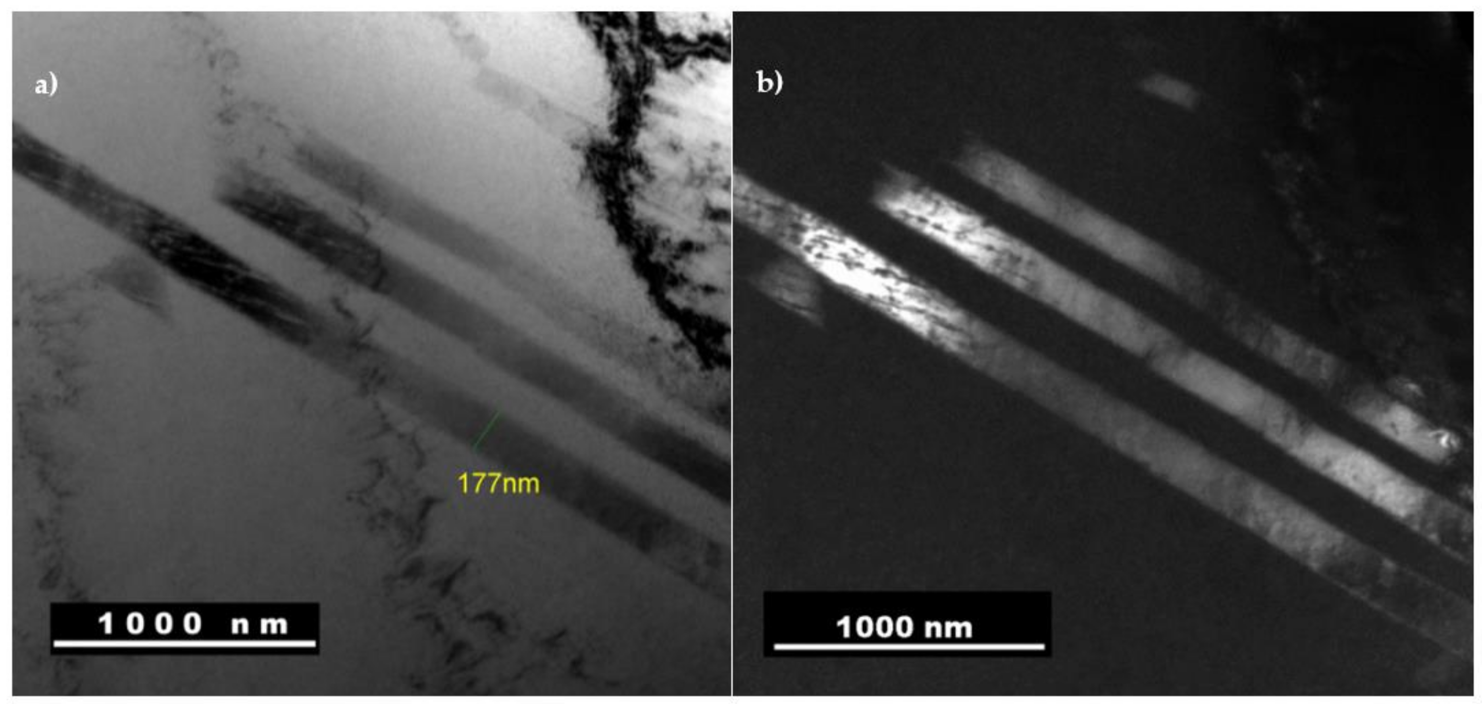
3.1. Initial Material Characterization

The micrograph in Figure 2a shows the microstructure of the as-swaged bars. It is possible to observe only the presence of the beta phase with a grain size average of 243 ± 13 µm. The rotary swaging process was adequate to dissolve the initial casting structure and promote the material’s complete recrystallization. In Figure 2b, is possible to observe the microstructure after solution heat treatment, consisting only of beta phase with an average grain size of 257 ± 27 µm with no traces of segregation from the solidified structure.

There was no significant grain growth after solution heat treating and the presence of the alpha phase was not detected by optical microscopy under any of the analyzed conditions.

Figure 3a presents the [012]_β SAED pattern of the solubilized condition (initial condition for compressive tests), showing diffraction spots of the omega phase, confirming the presence of the athermal omega phase in this condition. In Figure 3b,c the dark field of the athermal omega phase and beta phase distribution can be seen, respectively. A nanometric and disperse omega phase can be observed.

As previously reported by Reference [9], the isothermal omega phase continues the athermal omega phase transformation since beta stabilizers are continually rejected by the formed particles during aging. It has also been reported that high-pressure application and room-temperature deformation stabilizes the omega phase under certain circumstances [22,23]. The facts mentioned above are discussed in the literature. However, the omega phase precipitation (or its dissolution) during hot deformation has not been the object of research, perhaps due to the great complexity related to the interactions between dislocations and dispersed phases, as well as the occurrence of spinodal decomposition in alloys with a high content of molybdenum and its relationship to the presence of omega phase.

Figure 4 presents XRD spectra of three different initial conditions of TMZF before the compressive tests, as received (ingot), as rotary swaged, and rotary swaged and solubilized. From these spectra, it is possible to note a small amount of omega phase in the initial material (ingot) by the (002)_ω pronounced diffraction peak. Such an omega phase has been dissolved after rotary swaging. Although the omega phase has been detected on the solubilized condition using TEM-SAED pattern analysis, intense peaks of the corresponding planes have not appeared in XRD diffraction patterns. The absence of such peaks indicates that the high-temperature deformation process effectively promoted the dissolution of the isothermal omega phase, with only a very fine and highly dispersed athermal omega phase remaining, probably formed during quenching. It is also interesting to note that the most pronounced diffraction peak refers to the diffraction plane (110)_β, which is evidence of no occurrence of the twinning that is usually associated with the plane (002)_β.

3.2. Compressive Flow Stress Curves

The temperature of the sample deformed at 923 K and strain rate of 17.2 s⁻¹ is exhibited in Figure 5a. From this Figure, one can observe a temperature increase of about 100 K during deformation. During hot deformation, all tested samples exhibited adiabatic heating. Consequently, all the stress curves had to be corrected by Equation (1). The corrected flow stress is shown in Figure 5b in blue (dashed line) along with the stress curve before the adiabatic heating correction procedure.

The corrected flow stress curves are shown in Figure 6 for all tested strain rates and temperatures. The gray curves are the corrected stress values. The black ones were obtained from data interpolations of the previous curves between 0.02 and 0.8 of deformation. The interpolations generated a ninth-order function describing the average behavior of the curves and adequately representing all observed trends. The stress–strain curve of the sample tested at 1073 K and 17.2 s⁻¹ (Figure 6d) showed a drop in the stress value in the initial moments of the strain. This drop may be linked to the occurrence of deformation flow instabilities caused by adiabatic heating. Although this instability was not observed in the resulting analyzed microstructure, regions of deformation flow instability were calculated and are discussed later.

The true stress–strain values obtained using polynomial equations were also used to determine constitutive constants and develop a processing map at the total strain of 0.8.

From the curves for the samples deformed at the strain rate of 0.172 s⁻¹, it is possible to note discontinuous yielding at the initial deformation stage for the samples tested at 923 to 1023 K. The occurrence of discontinuous yielding has been related to the fast generation of mobile dislocations from grain boundary sources. The magnitude of such discontinuous yielding tends to be reduced by increasing the deformation temperature [24], as occurred in curves tested at 1073 to 1173 K, in which the observed phenomena have disappeared. The shape of the stress–strain curves points to precipitation hardening that occurs during deformation and dynamic recovery as the primary softening mechanism. All analyzed conditions have not shown a well-defined steady state of the flow stress. The recrystallization was delayed for higher deformation temperatures. It was inhomogeneously observed only in samples deformed at 0.172 s⁻¹ and 1173 K, as discussed in Section 3.6. Determination of the material’s constants was performed from the polynomial curves for each constitutive model, as detailed in the following.

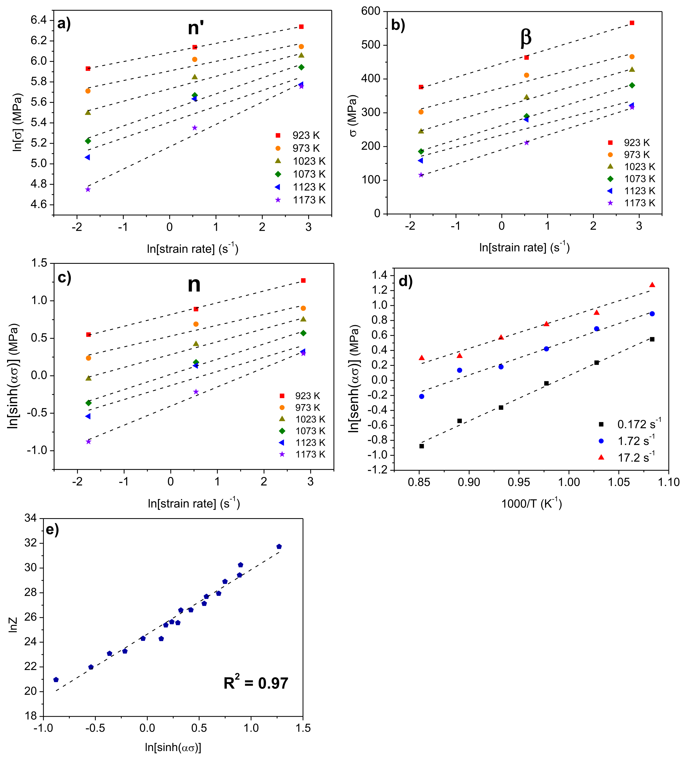
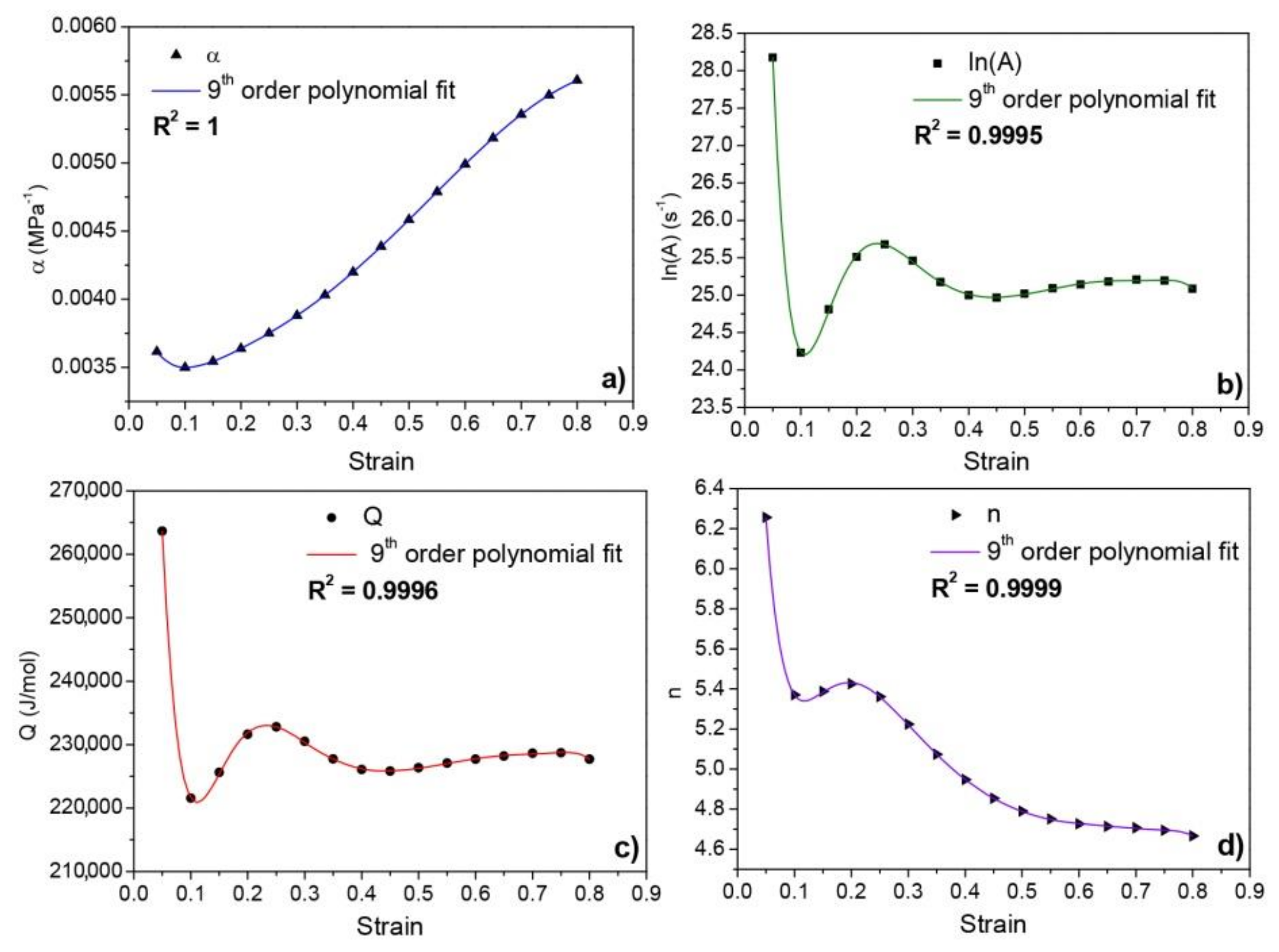
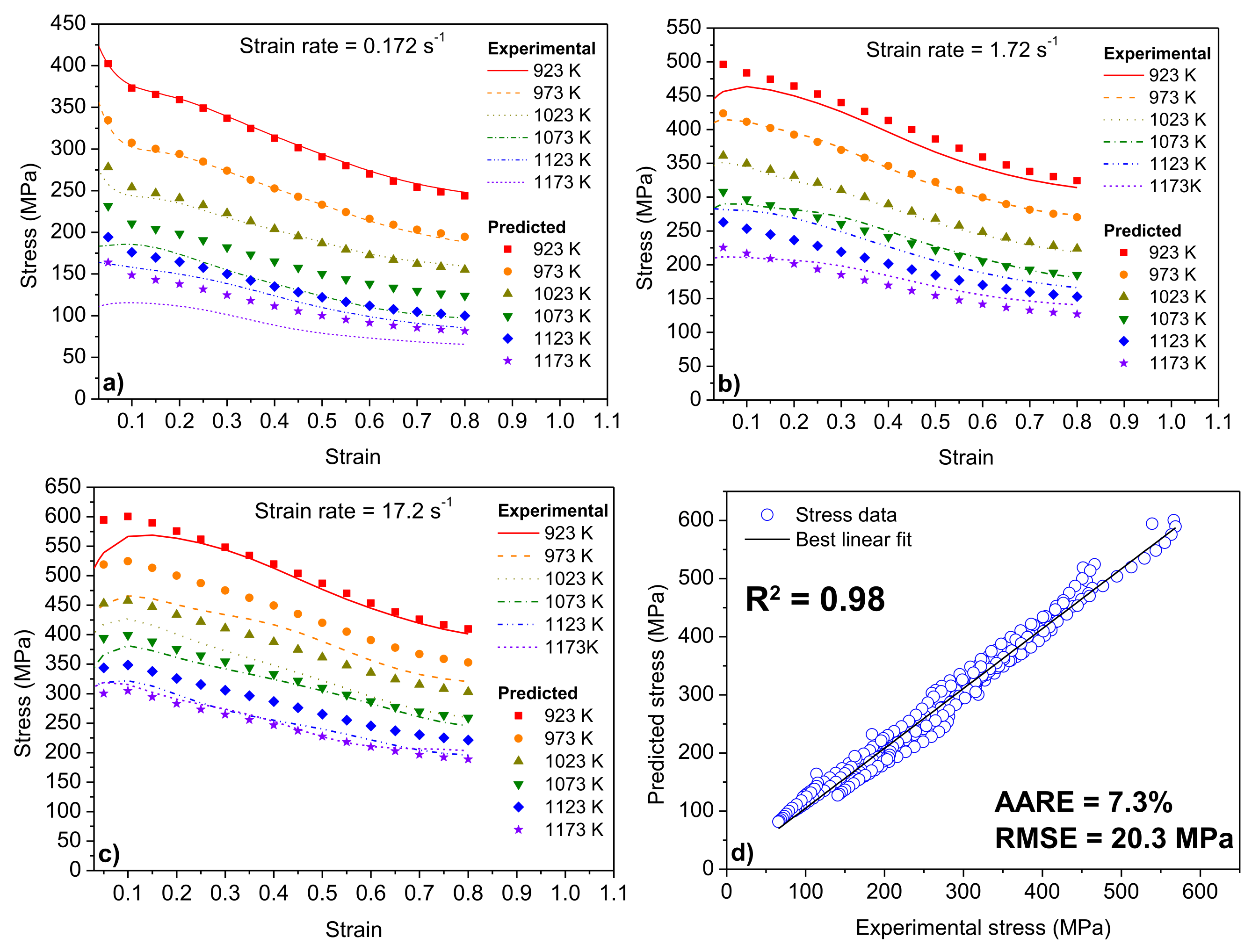
3.3. Arrhenius-Type Equation: Determination of the Material’s Constants

Data of each level of strain were fitted in steps of 0.05 to determine the constitutive constants. At a specific deformation temperature, considering low and high stress levels, we added the power law and exponential law (individually) into Equation (2) to obtain:

$$\dot{\epsilon }=A_1{\sigma }^{n^{\prime }}\exp \left[-Q/\left(RT\right)\right] \mathrm{and} \dot{\epsilon }=A_2\exp \left(\mathsf{\beta }\mathsf{\sigma }\right)\exp \left[-Q/\left(RT\right)\right]$$

(18)

here, the material constants $A_1$ and $A_2$ are independent of the deformation temperature. Taking the natural logarithm on both sides of the equations, we obtained:

$$ln\dot{\epsilon }=n^{\prime }\ln \sigma +\ln A_1-Q/\left(RT\right)$$

(19)

$$ln\dot{\epsilon }=\mathsf{\beta }\mathsf{\sigma }+\ln A_2-Q/\left(RT\right)$$

(20)

Substituting true stresses and strain rate values at each strain (in this plotting example, 0.1) into Equations (19) and (20) and plotting the $ln\sigma$ $\mathrm{vs}$. $ln\dot{\epsilon }$ and $\mathrm{vs}$. $ln\dot{\epsilon }$, values of $n^{\prime }$ and $\beta$ were obtained from the average value of slopes of the linear fitted data, respectively. At strain 0.1, shown in Figure 7a,b, the principal values of $n^{\prime }$ and $\beta$ were 7.194 and 0.0252, respectively. From these constants, the value of $\alpha$ was also determined, with a value of 0.0035 MPa⁻¹.

Since the hyperbolic sine function describes all the stress levels, the following relation can be used:

$$\dot{\epsilon }=A{\left[\sinh \left(\mathsf{\alpha }\mathsf{\sigma }\right)\right]}^n\exp \left[-Q/\left(RT\right)\right]$$

(21)

Taking the natural logarithm on both sides of Equation (21):

$$\ln \left[senh\left(\alpha \sigma \right)\right]=\frac{\ln \dot{\epsilon }}{n}+\frac{Q}{\left(nRT\right)}-\frac{lnA}{n}$$

(22)

For each particular strain, differentiating Equation (22), we obtained the following relation:

$$Q=Rn\frac{d\left\{\ln \left[senh\left(\alpha \sigma \right)\right]\right\}}{d\left(\raisebox{1ex}{$1$}\!\left/ \!\raisebox{-1ex}{$T$}\right.\right)}$$

(23)

As shown in Figure 7c,d, values of $n$ and $Q$ could be derived from the mean slopes of the $\left[sinh\left(\alpha \sigma \right)\right]$ $\mathrm{vs}$. $ln\dot{\epsilon }$ and the $ln\left[sinh\left(\alpha \sigma \right)\right]$ $\mathrm{vs}$. $1/T$. The value of Q and n were determined to be 222 kJ/mol and 5.4, respectively, by substituting the temperatures and true stress values at a determined strain (here, 0.1) obtained from each strain rate. Afterward, the mean value of $A$ could be obtained from the intercept of $\left[sinh\left(\alpha \sigma \right)\right]$ $\mathrm{vs}$. $ln\dot{\epsilon }$ plot, which was calculated to be 3742 × 10¹⁰ s⁻¹. The linear relation between parameter $Z$ (from Equation (5)) and $ln\left[sinh\left(\alpha \sigma \right)\right]$ is shown in Figure 7e.

From the values of the calculated constants for each strain level, a polynomial fit was performed according to Equation (6). The polynomial constants are presented in

Table 1. Polynomial fitting results of α, ln(A), Q, and n for the TMZF alloy.

$\mathit{\alpha }$	$\mathit{l}\mathit{n}\left(\mathit{A}\right)$	$\mathit{Q}$	$\mathit{n}$
$B_0=4.184\times {10}^{-3}$	$C_0=49.034$	$D_0=\mathrm{476,871.161}$	$E_0=10.589$
$B_1=-19.334\times {10}^{-3}$	$C_1=-740.767$	$D_1=-\mathrm{7,536,793.730}$	$E_1=-153.256$
$B_2=0.209$	$C_2=8704.626$	$D_2=\mathrm{88,012,642.533}$	$E_2=1799.240$
$B_3=-1.162$	$C_3=-\mathrm{53,334.268}$	$D_3=-\mathrm{539,535,772.259}$	$E_3=-\mathrm{11,205.292}$
$B_4=4.017$	$C_4=\mathrm{194,472.995}$	$D_4=\mathrm{1,972,972,002.321}$	$E_4=\mathrm{41,680.192}$
$B_5=-8.835$	$C_5=-\mathrm{447,778.132}$	$D_5=-\mathrm{4,558,429,469.855}$	$E_5=-\mathrm{98,121.148}$
$B_6=12.458$	$C_6=\mathrm{660,556.098}$	$D_6=\mathrm{6,745,748,811.780}$	$E_6=\mathrm{148,060.994}$
$B_7=-10.928$	$C_7=-\mathrm{607,462.488}$	$D_7=-\mathrm{6,219,011,380.735}$	$E_7=-\mathrm{139,080.466}$
$B_8=5.425$	$C_8=\mathrm{317,777.078}$	$D_8=\mathrm{3,258,916,319.726}$	$E_8=\mathrm{74,111.763}$
$B_9=-1.162$	$C_9=-\mathrm{72,301.922}$	$D_9=-\mathrm{742,230,347.439}$	$E_9=\mathrm{17,117.676}$

.

The material’s constant behavior with the strain variation is shown in Figure 8.

The highest values found for deformation activation energy were approximately twice the value for self-diffusion activation energy for beta-titanium (153 kJ·mol⁻¹) and above the values for beta alloys reported in the literature (varying within a range of 130–175 kJ·mol⁻¹) [24], as can be seen in Figure 8c. This model is based on creep models. Therefore, it is convenient to compare the values of the determined constants with deformation phenomena found in this theory. High values of activation energy and n constant (Figure 8d) are reported to be typical for complex metallic alloys, being in the order of 2 to 3 times the $Q$ values for self-diffusion of the base metal’s alloy. This fact is explained by the internal stress present in these materials, raising the apparent energy levels necessary to promote deformation. However, when considering only the effective stress, i.e., the internal stress subtracted from the applied stress, the values of $Q$ and n assume values closer to the physical models of dislocation movement phenomena (${\sigma }_{eff}={\sigma }_{apl}-{\sigma }_{int})$. Thus, when the values of $n$ take values above 5, it is likely that there are complex interactions of dislocations with precipitates and dispersed phases in the matrix, formation of tangles, or substructure dislocations that contribute to the generation of internal stresses in the material’s interior [25]. For higher deformation levels (greater than 0.5), the values of $Q$ and $n$ were reduced and appear to have stabilized at values of approximately 230 kJ and 4.7, respectively. At this point of deformation, the dispersed phases probably no longer efficiently delayed the dislocation’s movement.

The experimental flow stress (lines) and predicted stress by the strain-compensated Arrhenius-type equation for the TMZF alloy are shown in Figure 9a–c for the different strain rates (dots) and in Figure 9d is possible to see the linear relation between them. As mentioned, the n constant values presented for this alloy stabilized at values close to 4.7. This magnitude of $n$ value has been associated with dislocation movement by climbing mechanisms. In contrast, values above 5 have been related to internal stresses related to complex dislocation interactions with dispersed phases [26]. Therefore, a more significant presence of internal stress was observed at the initial stages of deformation, with its action reduced when larger deformation levels were reached. The presence of the athermal omega phase and β spinodal phases (which will be discussed later) were probably responsible for the appearance of the observed internal stresses.

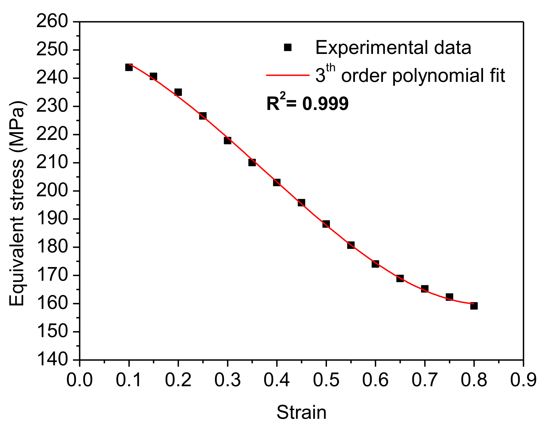
3.4. Modified Johnson–Cook Model

For determination of the material constants in the first term of Equation (10), a polynomial fit was applied to the reference curve, which was determined to be at 1023 K and 0.172 s⁻¹. The polynomial constant values of the third-order equation were found to be: $A_1$ = 252.49 MPa, $B_1$ = −47.12 MPa, $B_2$ = −295.39 MPa, and $B_3$ = 262.08 MPa. The fitted polynomial curve can be seen in Figure 10.

For $C_1$ determination, when the deformation temperature is the reference one, Equation (9) becomes:

$$\sigma =\left(A_1+B_1\epsilon +B_2{\epsilon }^2+B_3{\epsilon }^3\right)(1+C_{1}ln{\dot{\epsilon }}^{*})$$

(24)

By rearranging the above relation, it is possible to obtain:

$$\frac{\sigma }{\left(A_1+B_1\epsilon +B_2{\epsilon }^2+B_3{\epsilon }^3\right)}=\left(1+C_{1}ln{\dot{\epsilon }}^{*}\right)$$

(25)

From Equation (25), it is possible to determine the value of constant $C_1$ as the linear fit slope of $\frac{\mathsf{\sigma }}{\left({\mathrm{A}}_1+{ \mathrm{B}}_1\mathsf{\epsilon }+{ \mathrm{B}}_2{\mathsf{\epsilon }}^2+{ \mathrm{B}}_3{\mathsf{\epsilon }}^3\right)}$ $\mathrm{vs}$. $ln{\dot{\epsilon }}^{*}$. The products $\frac{\mathsf{\sigma }}{\left({\mathrm{A}}_1+{ \mathrm{B}}_1\mathsf{\epsilon }+{ \mathrm{B}}_2{\mathsf{\epsilon }}^2+{ \mathrm{B}}_3{\mathsf{\epsilon }}^3\right)}$ of the eighteen experimental flow stress points were plotted against $ln{\dot{\epsilon }}^{*}$ (as shown in Figure 11) (using eight strain data points varying between 0.1 and 0.8 for each strain rate/temperature combination), and $C_1$ value was determined to be 0.173.

To determine ${\lambda }_1$ and ${\lambda }_2$, which are related to the strain rate effect, a reorganization of Equation (10) is done as follows:

$$\frac{\sigma }{\left[\left(A_1+B_1\epsilon +B_2{\epsilon }^2+B_3{\epsilon }^3\right)\ast \left(1+C_{1}ln{\dot{\epsilon }}^{*}\right)\right]}=e^{\left({\lambda }_1+{\lambda }_{2}ln{\dot{\epsilon }}^{*}\right)\ast \left(T-T_{ref}\right)}$$

(26)

Applying the natural logarithm in both sides of Equation (26), one may obtain the following Equation:

$$ln\left\{\frac{\sigma }{\left[\left(A_1+B_1\epsilon +B_2{\epsilon }^2+B_3{\epsilon }^3\right)\ast \left(1+C_{1}ln{\dot{\epsilon }}^{*}\right)\right]}\right\}=\left({\lambda }_1+{\lambda }_{2}ln{\dot{\epsilon }}^{*}\right)\ast \left(T-T_{ref}\right)$$

(27)

The relation between the first term of Equation (27) and $\left(T-T_{ref}\right)$ is obtained from the different strains, strain rates, and temperatures. Equation (27) can be expressed, using the relation λ = λ₁ + λ₂ln$\dot{\epsilon }$*, as:

$$ln\left\{\frac{\sigma }{\left[\left(A_1+B_1\epsilon +B_2{\epsilon }^2+B_3{\epsilon }^3\right)\ast \left(1+C_{1}ln{\dot{\epsilon }}^{*}\right)\right]}\right\}=\lambda \left(T-T_{ref}\right)$$

(28)

For the three different strain rates and temperatures tested, the value of $\lambda$ was determined as the slope of the linear fit shown in Figure 12.

From Figure 12, we obtained the values of ${\lambda }_{\left({\dot{\epsilon }}^{*}=0.1\right)}=-0.0051$, ${\lambda }_{\left({\dot{\epsilon }}^{*}=1.0\right)}=-0.0031,$ and ${\lambda }_{\left({\dot{\epsilon }}^{*}=10\right)}=-0.0028$. Values of $\lambda$ were plotted against $\ln \left({\dot{\epsilon }}^{*}\right)$ to obtain the values of λ₁ and λ₂. They are the interception of the linear fit and the slope, respectively, as shown in Figure 13.

From Figure 13, the constants ${\lambda }_1$ and ${\lambda }_2$ were determined to be −0.00479 and 0.0004959, respectively. Finally, substituting the determined constants in Equation (10), the modified Johnson–Cook equation, the obtained equation to predict the flow stress of TMZF alloy is expressed in Equation (29).

$$\sigma =\left(252.49-47.12\epsilon -295.39{\epsilon }^2+262.08{\epsilon }^3\right)\left(1+0.17 ln\frac{\dot{\epsilon }}{0.172}\right)\exp \left[\left(-0.005+0.0005\right)\left(T-1023\right)\right]$$

(29)

The experimental flow stress (lines) and predicted stress by the modified JC model for the TMZF alloy are shown in Figure 14a–c for the different strain rates (dots), and in Figure 14d, it is possible to see the linear relation between them.

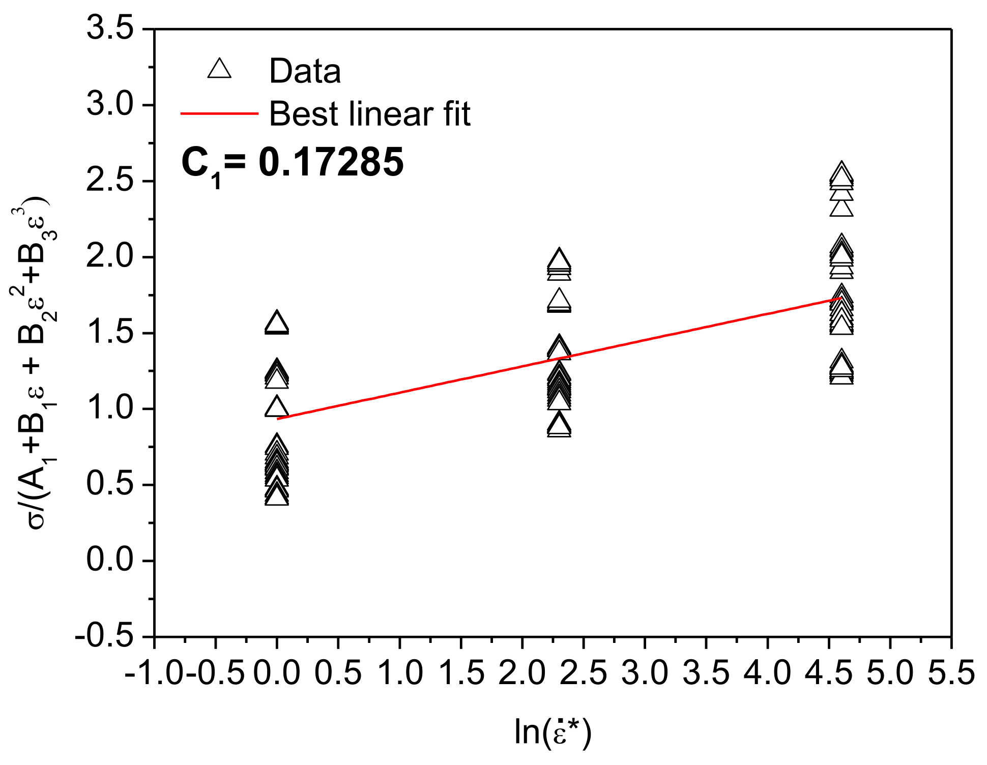
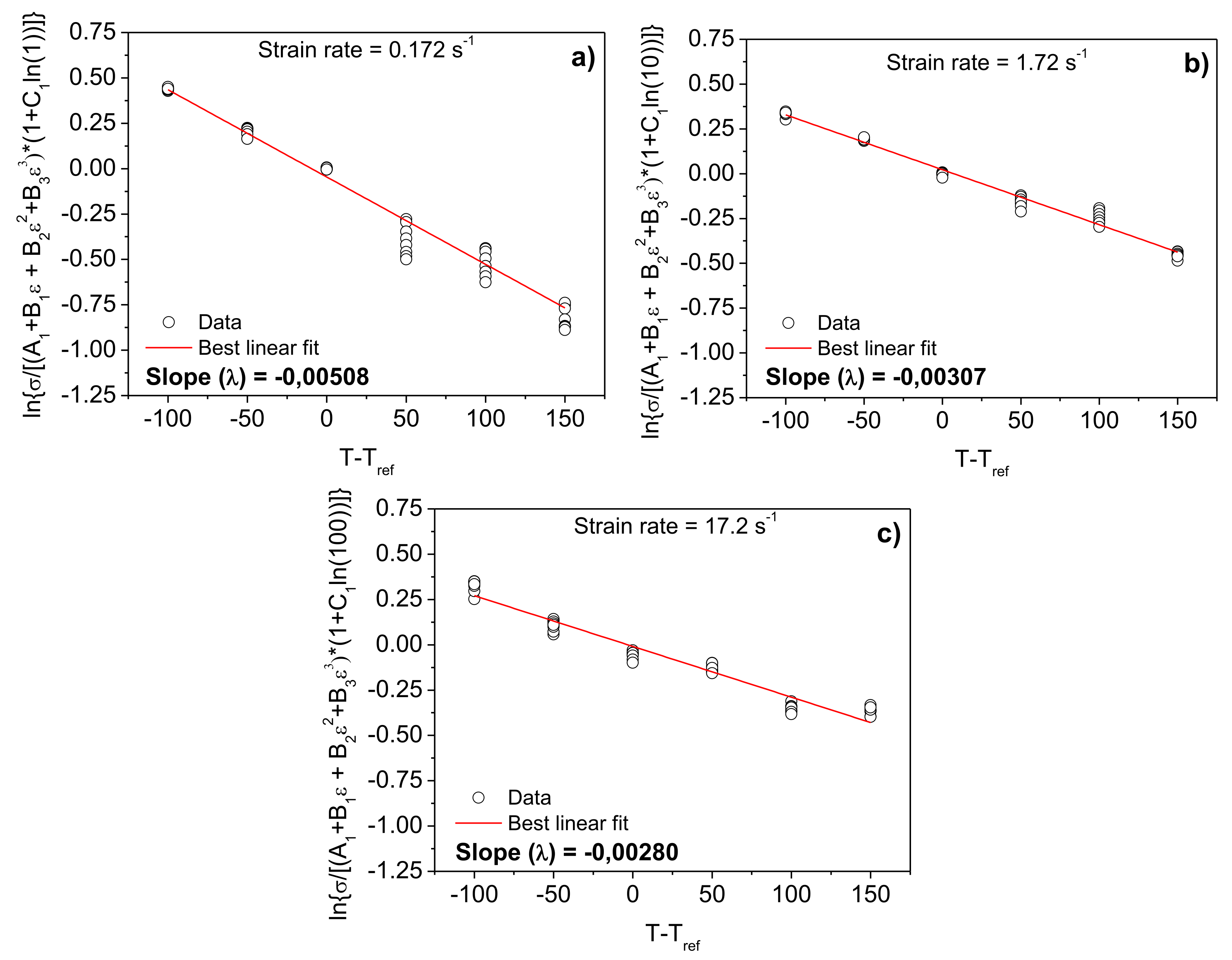
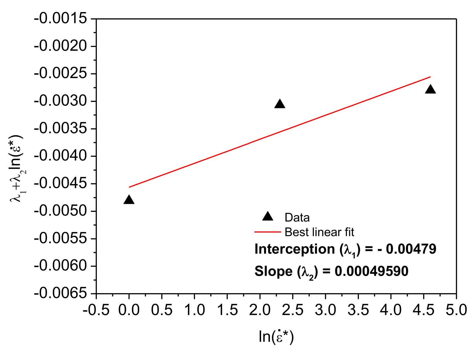
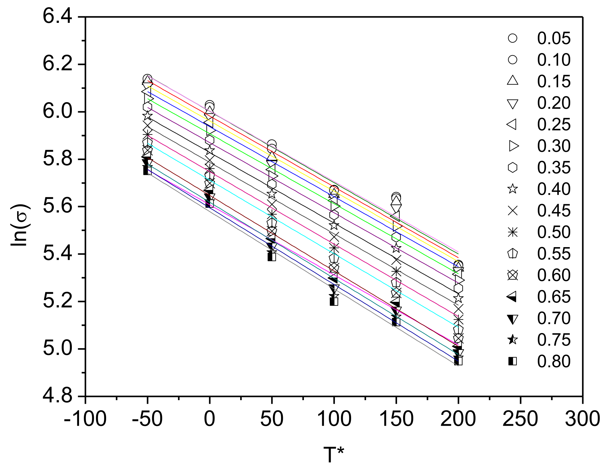
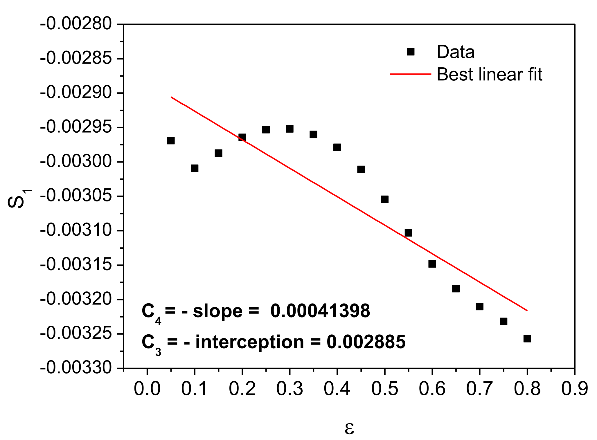
3.5. Modified Zerilli–Armstrong Model

Aiming to determine the material constants of the first term of Equation (12), a polynomial fit was applied to the reference curve, which was determined to be at 973 K and 1.72 s⁻¹. The polynomial constant values of the third-order equation were found to be: $A_1$ = 546.99 MPa, $B_1$ = −646.69 MPa, $B_2$ = −11.406 MPa, and $B_3$ = 418.18 MPa. The fitted polynomial curve can be seen in Figure 15 below:

The slope value of the plot of $ln\left(\sigma \right)$ vs. $T^{*}$ provides $S_1=-\left(C_3+C_4\epsilon \right)$ to determine C3 and C4 values, as shown in Figure 16.

Plotting $S_1$ vs. ε (Figure 17), the values of $C_3$ and $C_4$ were determined, being the interception and slope, respectively. The values of the constants were $C_3$ = 0.003 and $C_4$ = 0.0004.

From the slope of the plot of $\ln \left(\sigma \right)$ vs. $\ln \left({\dot{\epsilon }}^{*}\right)$, the value of $S_2$ was obtained. Plotting the $S_2$ vs. $T^{*}$(for all strain levels) and using the relation $S_2=C_5+C_6{T}^{*}$, $C_5$ and $C_6$ were obtained from the intercept’s average value and slope of the linear fit of all strains, respectively. The linear fit of $S_2$ is shown in Figure 18. The values of $C_5$ and $C_6$ were determined to be 0.11 and 0.0005.

For better predictability of the constitutive equation, these constants were optimized by a non-linear regression method. The improved values were found to be 0.124 and 0.0004 for C₅ and C₆, respectively. The resulting modified ZA equation is shown in Equation (30).

$$\sigma =\left(546.99{\epsilon }^3 - 646.69{\epsilon }^2 - 11.41\epsilon + 418.18\right)\exp \left\{-\left(0.003+0.0004\epsilon \right)T^{*}+\left(0.12+0.0004T^{*}\right)ln{\dot{\epsilon }}^{*}\right\}$$

(30)

The experimental flow stress (lines) and predicted stress by the modified ZA model for the TMZF alloy are shown in Figure 19a–c for the different strain rates (dots), and in Figure 19d, it is possible to see the linear relation between them.

If one compares the models, it can be observed that all models can satisfactorily predict the flow stress behavior. However, the modified ZA model results in a significant error and poor predictability for the lowest deformation temperatures. Hence, this model is the least suitable for modeling the behavior under hot deformation for the TMZF alloy. The modified JC model slightly improved the predictability compared with the strain-compensated Arrhenius-type equation. Nevertheless, the use of Arrhenius equations is suggested because, as discussed above, the physical meaning of the obtained equation constants can be correlated with dislocation’s movement mechanisms. The received activation energy parameter may be associated with some similarly obtained data of alloys to predict the softening mechanism, therefore, allowing the physical description of metallurgical events occurring during hot working.

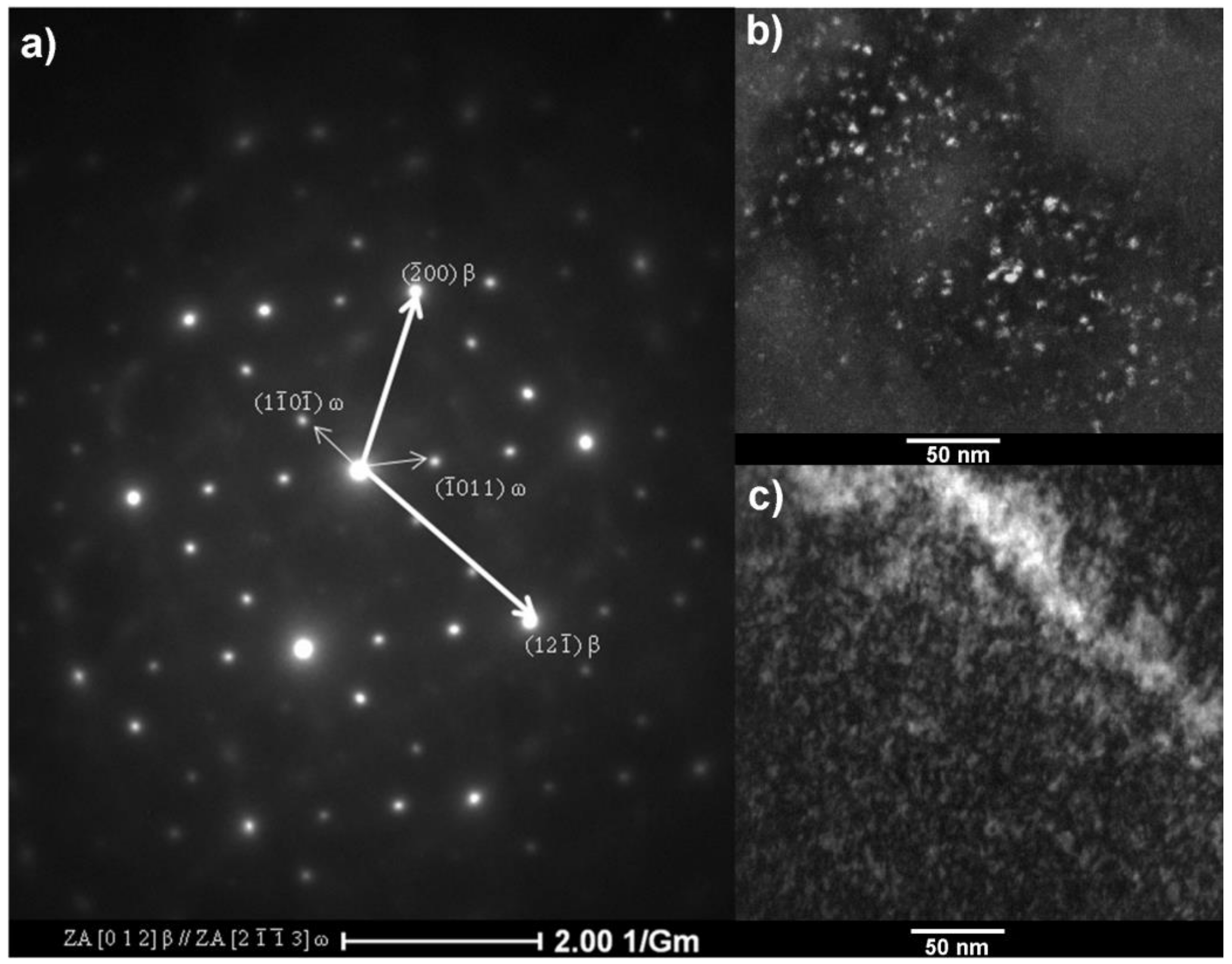
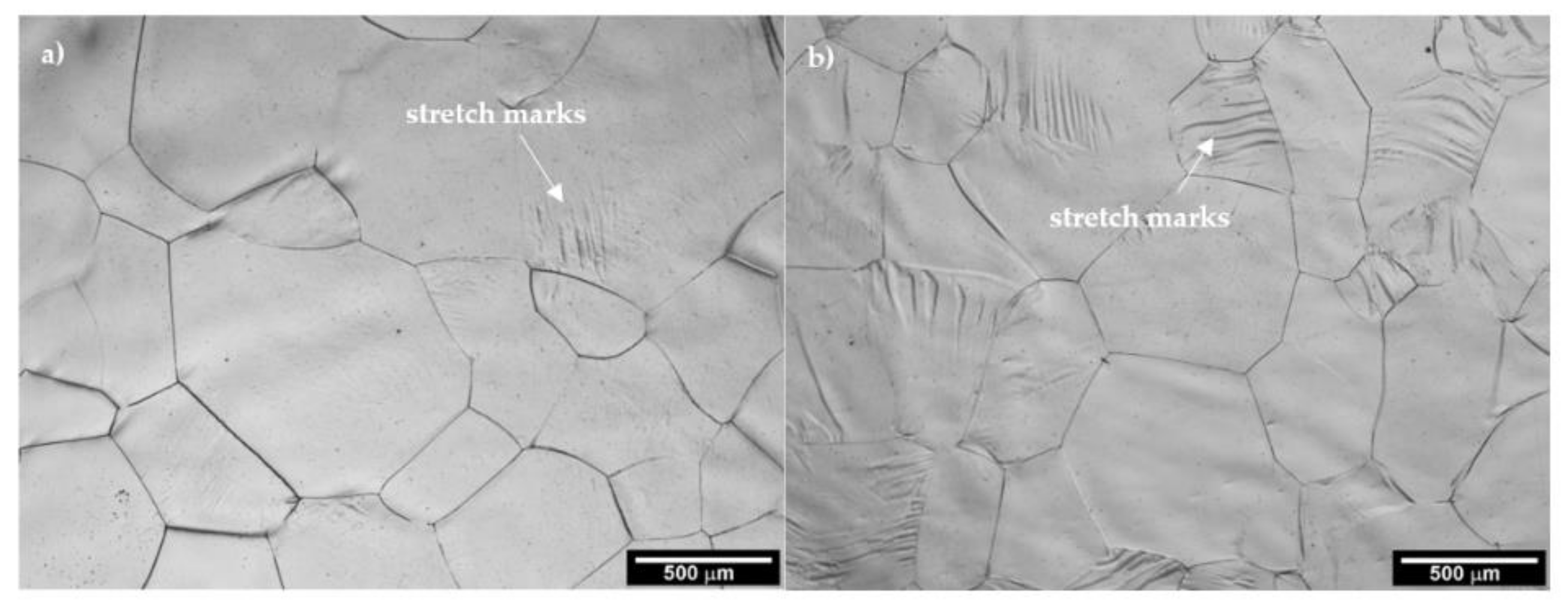
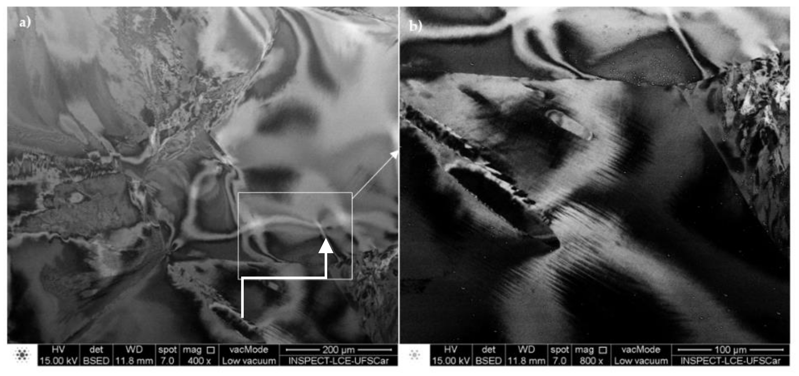
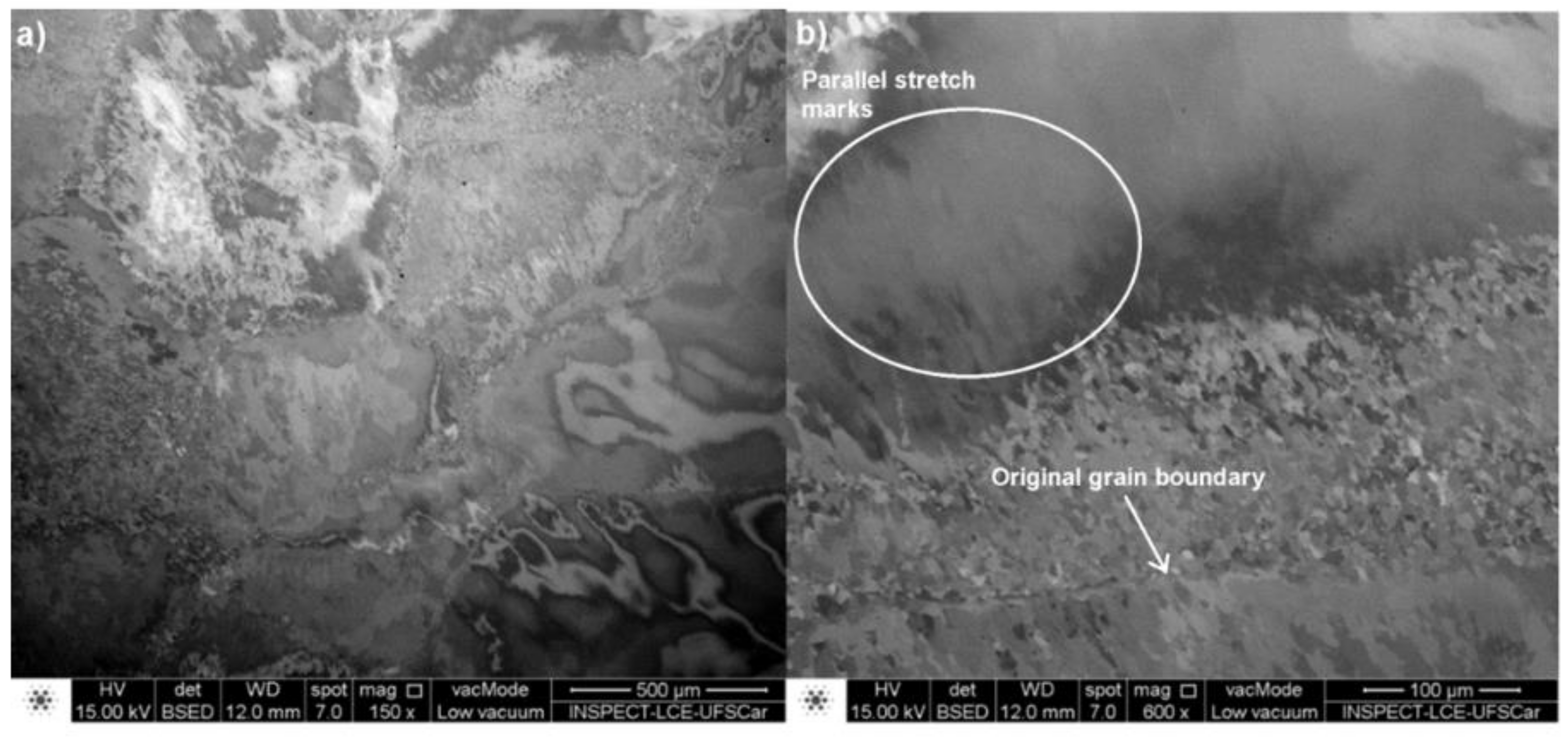
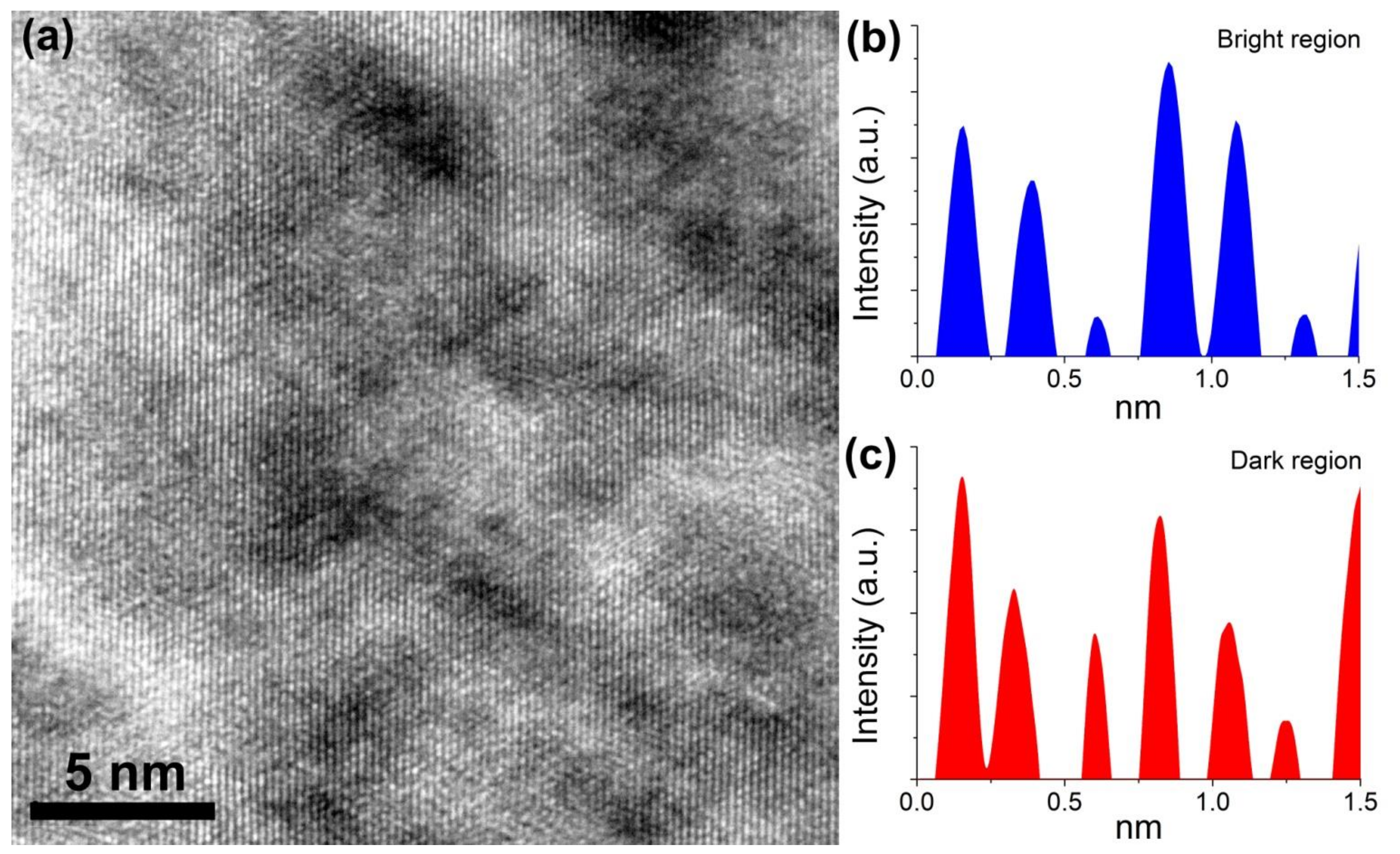
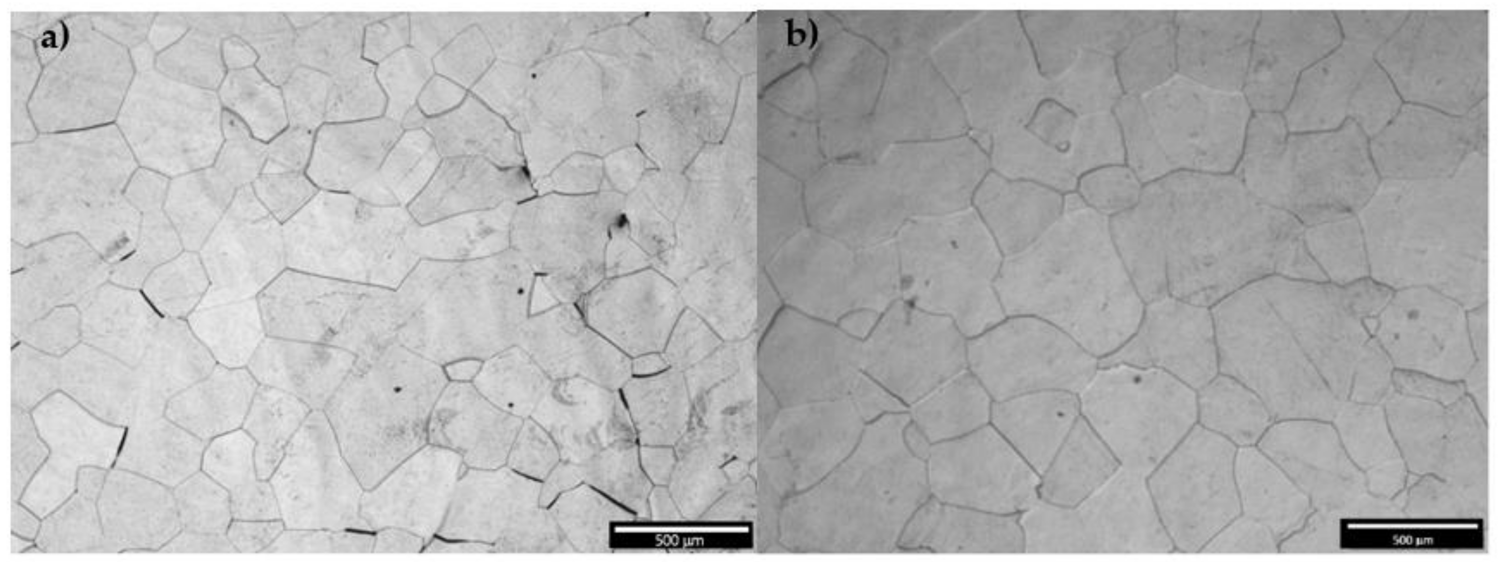
3.6. Microstructure Characterization after Processing

The microstructures of deformed samples at 923 K are shown in Figure 20. In Figure 20a, it is possible to see the resulting microstructure of the sample deformed at 923 K and 0.172 s⁻¹. There was no dynamic recrystallization during the hot deformation, and parallel stretch marks can be seen in the grain’s interior. Stretch marks become more prominent by increasing the strain rate to 17.2 s⁻¹ (Figure 20b), which is similar to the macro mechanical twinning evidence.

High-contrast BSED analysis was performed by SEM on the sample shown in Figure 20b to investigate the stretch marks detected by optical micrographs. This analysis provides information about crystallographic orientation since EBSD analysis was not possible due to the highly deformed condition of the sample, which resulted in a poor-quality Kikuchi signal and made EBSD analysis unfeasible.

In Figure 21a,b it is possible to observe stretch marks in two different magnifications, confirming that they are results of differences in crystalline orientation, indicating a possible occurrence of micrometric-order mechanical twinning in the grain’s interior for the sample deformed at 923 K and 17.2 s⁻¹.

For the sample deformed at 923 K and 0.172 s⁻¹, the stretch marks shown in Figure 20a were much less pronounced than those observed for the higher strain rate by optical micrography. Aiming to confirm if these marks originated from the mechanical twinning occurrence, an automated crystal orientation analysis was performed inside one original beta grain of the TMZF sample deformed at 923 K and 0.172 s⁻¹. Figure 22 presents the resulting map. From this Figure, one may notice two different zones with parallel marks with different crystallographic orientations and sizes but micrometric-order sizes.

The measured thickness of one of the stretch marks of Zone 1 in Figure 22 was found to be 177 nm, as can be seen in Figure 23a, where it is possible to observe a TEM bright field image of the analyzed zones, and in (b), the dark field image of the corresponding region is shown. Figure 24a shows a virtual bright field image of the same analysis location. A line was traced along an AB axis to measure the misorientation crystallographic profile, plotted along with the distance. Figure 24b shows the resulting misorientation profile, where it is possible to note that crystallographic orientation fluctuated in steps of 60° along the AB line, corresponding to the {112} <111>-type deformation twinning and confirming that the parallel marks resulted from the mechanical twinning occurrence.

A line misorientation profile of the AB axis in Zone 2 (region shown in Figure 22) is shown in Figure 25b. The mechanical twins in this zone were found to be of nanometric order, indicating that, although not detectable by optical microscopy, the occurrence of twinning was a vital deformation mechanism for this alloy.

Analyzing the optical micrographs of the samples deformed at 1173 K in Figure 26a, is possible to observe the occurrence of dynamic recrystallization at $\dot{\epsilon }=0.172$ s⁻¹, in which serrated grain boundaries resulting from a bulging mechanism are evident. Such temperature and strain rate were the only combination of processing parameters in which recrystallization occurred. It is possible to note, by microstructural analysis, that only a few grains have shown recrystallization in the grain interior, with the recrystallization process being inhomogeneous, preferably occurring in regions near the grain boundaries, which were serrated due to the occurrence of CDRX. After increasing the strain rate to 17.2 s⁻¹, there was no recrystallization. The primary softening mechanism continued to be the dynamic recovering, as shown in Figure 26b.

High-contrast BSED analysis of the sample deformed at 1173 K and $\dot{\epsilon }$= 0.172 s⁻¹ (same sample of Figure 26a) is shown in Figure 27 at two different magnifications, with which we aimed to show microstructural characteristics. It is possible to note the continuous dynamic recrystallization (CDRX) process, especially in grain boundaries, preceded by a strong recovering process, as pointed out in previously analyzed literature. The new recrystallized grains at the original grain boundaries were 10 to 20 micrometers size. Stretch marks were found in the initial beta grains’ interiors, as shown in Figure 27b, which probably resulted from mechanical nano-twinning deformation, as detected in the sample deformed at the same temperature and higher strain rate.

Figure 28 presents a high-contrast BSED image taken from a sample deformed at 1173 K and 17.2 s⁻¹. In this figure, one may observe that, although there is no evidence of dynamic recrystallization, the occurrence of parallel marks (evidence of nano-twinning) and macro mechanical twinning became even more prominent.

In general, it can be noted that there was a delay in recrystallization occurrence. It was heterogeneous in the sample tested at the highest temperature and lower strain rate when it occurred. The dynamic recovery, the predominant softening mechanism, and twinning were vital deformation mechanisms for all the temperatures used in hot compression tests.

The most common effect of solutes is the prevention of recrystallization. The quantitative effect of a solute on the recrystallization occurrence depends on the specific solvent/solute pair, acting in high concentrations to delay recrystallization, raising the temperature at which it occurs. The delay at the beginning of recrystallization observed for this alloy can be explained by the high concentration of alloying elements (Mo, Zr, and Fe), which, due to similar atomic sizes to that of titanium, were found in solid solution in the beta matrix. Atoms in solid solution can delay both the start of nucleation and the growth rate of the recrystallized grains. The effect of atoms in solid solution in multi-elemental alloys has not been quantified. However, most experimental work suggests that the primary influence of solutes is on the mobility of grain boundaries [27].

Lucci et al. [27] studied the effect of the addition of substitutional transition elements on the recrystallization behavior and stored energy in binary copper alloys. The authors concluded that small additions increase the recrystallization rate and the amount of accumulated energy or driving force for its event (depending on the element’s atomic volume due to elastic interactions). However, they always delay recrystallization in high concentrations. At the same time, the stored energy can be increased or decreased, depending on the type of solute. In this case, the delay effect depends on the binding energy between the solute and contour.

In her thesis, Trump [28] reported that the study of recrystallization kinetics for steels under the effect of solute is widespread. However, for titanium, studies quantifying these effects are minimal. Surveying the impact of the addition of aluminum on the titanium static recrystallization kinetics, Trump discussed the causes of the observed reduction in grain boundary mobility promoted by additions of 0% to 7% in weight of Al, which caused a delay in time for 50% recrystallization from 1 to 1240 min. Since the delay in grain growth kinetics with increasing solute concentration is generally attributed to the solute drag effect, most researchers have tried to explain this phenomenon by assuming that solutes segregate at the grain boundaries causing their drag delay. However, this segregation has rarely been confirmed experimentally, being observed via microscopy only in alloys with diluted solute concentrations, which is explained via kinetic and thermodynamic mechanisms.

The kinetic effect is based on the difference between the diffusivity of the solute and matrix atoms. Assuming that atoms in solution located at grain boundaries have a lower diffusivity in the matrix than the solvent atoms, grain boundaries need to drag these atoms in solution to move, thus reducing the mobility of the boundary. The thermodynamic effect reduces the boundary energy due to the segregated solute atoms at the contours, reducing the driving force for grain growth. Given these two mechanisms, it would be expected that the higher the solute concentration in the alloy, the greater the concentration of the elements at grain boundaries and the greater the solute drag effect in the grain growth kinetics. However, this fact was not observed in her work using transmission electron microscopy and energy-dispersive spectroscopy techniques. After discussing the existing interactions and theories to explain the non-occurrence of segregation in the Ti-Al alloy, the author concluded that the interaction between solute atoms for high-concentration alloys should be considered. They justified this conclusion by observing that in solutions with solutes at concentrations close to the solubility limit, it is energetically favorable that the atoms in the solution stay close to each other. Precipitation will only occur if the solubility limit is exceeded. In this way, solute atoms are increasingly attracted to each other and segregation becomes energetically unfavorable in the grain boundary regions. Hence, atoms in solution repel the boundaries instead of being attracted to them, i.e., energy segregation becomes positive instead of negative (when segregation occurs). In this way, the effect of the atoms in solution in reducing grain boundaries’ mobility is attributed to the fact that the boundaries must push or repel the solute atoms to move [28].

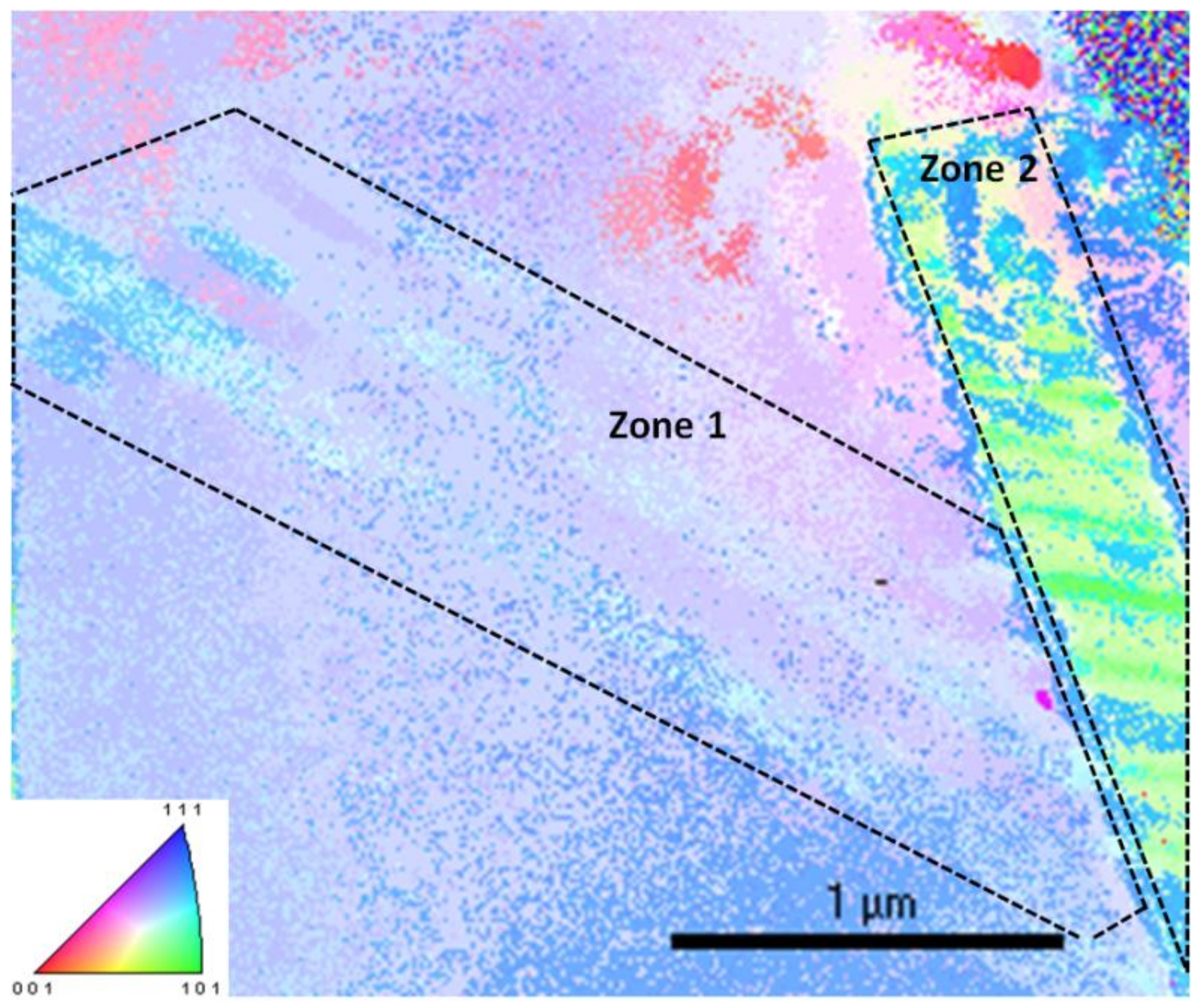
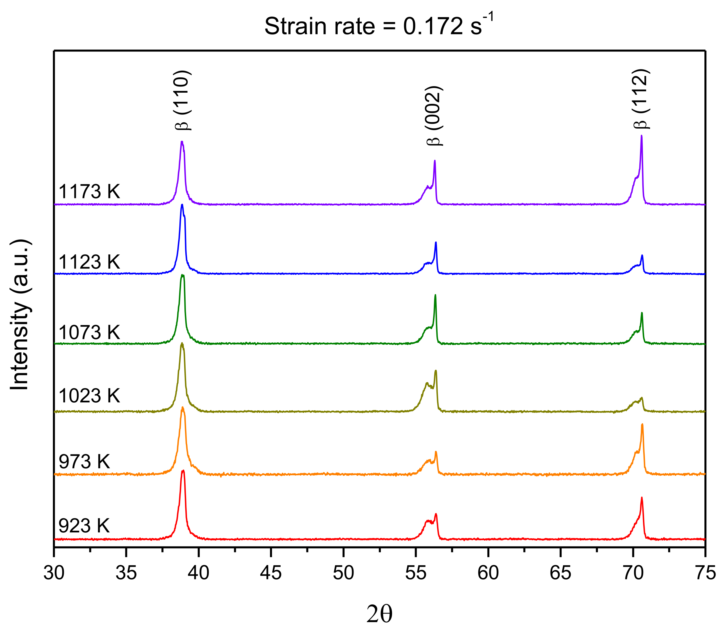
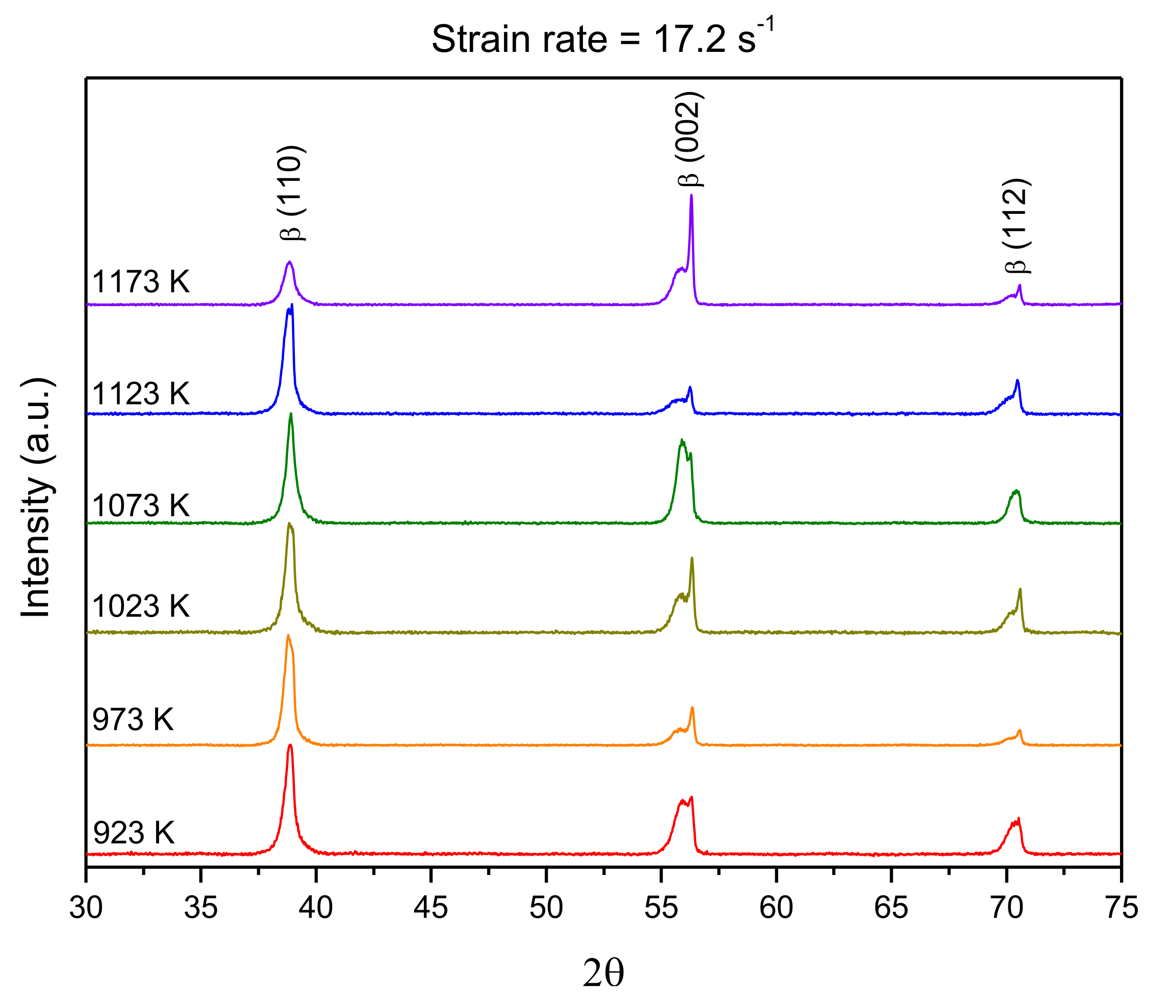
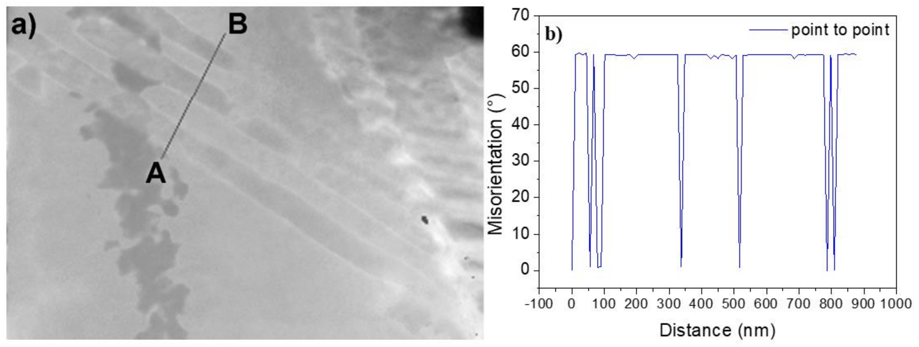
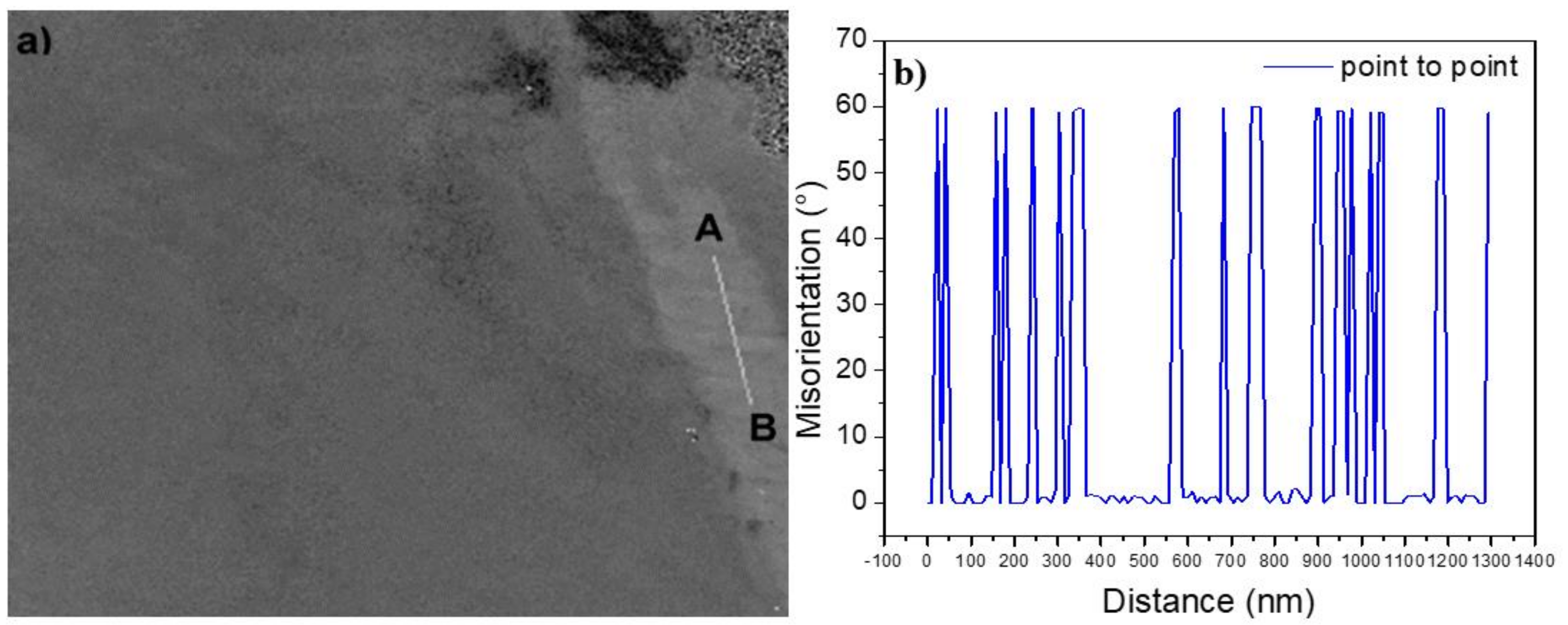
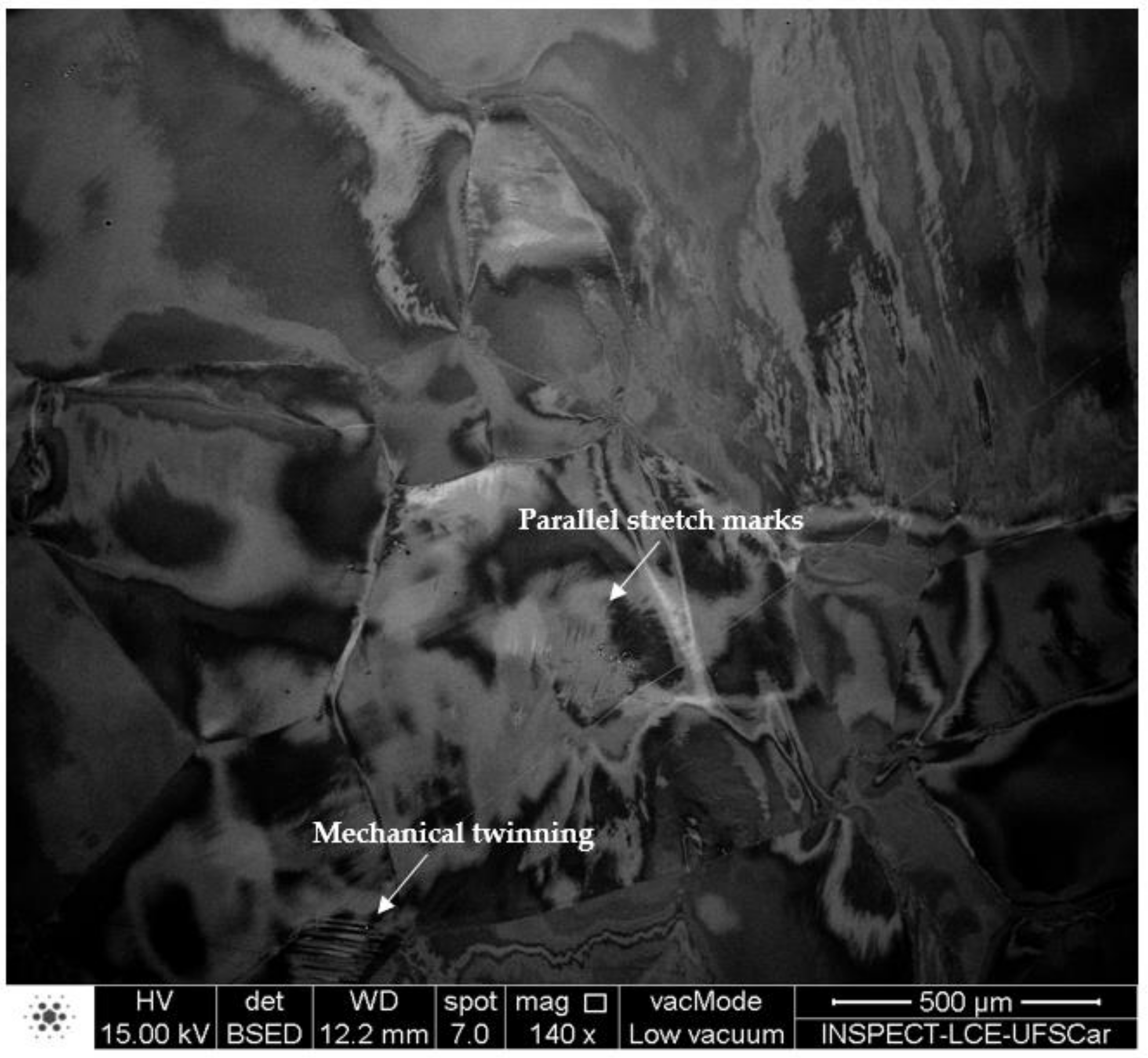
3.7. Structural Analysis

X-ray diffractograms of TMZF samples deformed at $\dot{\epsilon }=0.172$ s⁻¹ and $\dot{\epsilon }=17.2$ s⁻¹ at different temperatures are presented in Figure 29 and Figure 30, respectively. The only beta phase was found to be present in all the analyzed conditions. The beta phase peaks showed characteristics of duplicity, being more evident at the (002)_β and (112)_β diffraction planes, pointing to a possible occurrence of spinodal decomposition of the beta phase during hot deformation in all tested conditions.

The spinodal decomposition was confirmed by TEM analysis, as shown in Figure 31. Figure 31a presents a high-resolution TEM image (HR-TEM) obtained along the zone axis [110]_β for a sample processed at ε = 17.2 s⁻¹ at 1023 K. In this Figure, one may observe bright and dark regions. Line intensity profiles of bright and dark areas are presented in Figure 31b,c respectively. These profiles reveal equally spaced peaks corresponding to interplanar distances. More peaks were observed in the dark region graph than in the bright one, indicating that the dark region possessed a smaller interplanar distance than the bright. Calculations gave average values of ~0.23086 ± 0.00034 nm and ~0.22985 ± 0.00048 nm for the interplanar distances of bright and dark regions, respectively.

For the two strain rates analyzed by XRD, it is possible to observe a more pronounced change in the shape of the beta phase diffraction peaks at temperatures above and below the phase transition temperature, mainly in the peak referring to the plane (112)_β. In general, it is possible to observe that the sharpest peak was displaced to larger diffraction angles. Comparing the diffraction patterns obtained with those obtained in the initial material (Figure 4), a strong texturization of the material can be observed. The phase transformation from β₁ to β₂ by spinodal decomposition explains the increase in mechanical strength at the initial moments of deformation observed in samples tested above the beta transition temperature. The precipitation of the β₂ phase increased with deformation and, together with precipitate remnants of the omega phase, dynamically pinned dislocations much more intensely than a single-phase material, leading to the very accentuated work hardening observed in the initial deformation steps.

Furthermore, the fact that the XRD peaks demonstrated the occurrence of an almost complete transformation indicates that a considerable amount of the alloying elements entered solid solution, increasing the effect of solute drag during deformation. This fact led the alloy to present a delay in the occurrence of recrystallization, with dynamic recovery being quite accentuated, as mentioned above, explaining the small recrystallization observed only under specific conditions observed under optical microscopy.

In addition, once again, it is noted that there was no increase in width at the peak’s half-height. This behavior indicates no recrystallization, or it was not enough to appear on diffraction patterns. The strain did not accumulate even at low temperatures, showing a very intense dynamic recovery process.

The movement of the peaks to larger diffraction angles compared to the forged and homogenized samples (Figure 4) also indicates the occurrence of twinning, which also favored the formability of the alloy.

The spinodal decomposition evidence corroborates the high values found for the Arrhenius equation’s constants, $n$ and $Q$, pointing to the existence of highly dispersed coherent phases impacting the dislocations’ movement. Spinodal decomposition and twinning mechanisms led to the emergence of internal stresses at the initial stages of plastic deformation.

4. Conclusions

The microstructural analysis led to the conclusion that the primary softening mechanism of the TMZF alloy, within the range of temperatures and strain rates analyzed, was DRV.

CDRX was found to operate at the higher analyzed temperature and lower strain rate, where bulging mechanisms were observed.

The TMZF’s high solute content, which led to a high value of SFE, promoted the prevalence of DRV mechanisms and delayed CDRX to higher values of temperature deformation.

Micro- and nanometric order mechanical twinning were an essential mode of deformation for this alloy (decreasing the $m$ value and power dissipation efficient parameter). Twinning was accompanied by the athermal omega phase and spinodal phases in the formation of complex pinning atmospheres, which interacted with dislocations during the initial stages of plastic deformation, leading to an increase in the Arrhenius-calculated constant values $Q$ and $n$.

The phenomenological constitutive equations of the J-C and strain-compensated Arrhenius-type equation exhibited better flow stress predictability than the ZA model.

References

1. Soundararajan, S.R.; Vishnu, J.; Manivasagam, G.; Muktinutalapati, N.R. Titanium Alloys–Novel Aspects of Their Manufacturing and Processing; Motyka, M., Ziaka, W., Sieniawski, J., Eds.; IntechOpen Limited: London, UK, 2018. [Google Scholar]
2. Quadros, F.D.F.; Kuroda, P.A.B.; Sousa, K.D.S.J.; Donato, T.A.G.; Grandini, C.R. Preparation, structural and microstructural characterization of Ti-25Ta-10Zr alloy for biomedical applications. J. Mater. Res. Technol. 2019, 8, 4108–4114. [Google Scholar] [CrossRef]
3. Song, Y.H.; Kim, M.K.; Park, E.J.; Song, H.J.; Anusavice, K.J.; Park, Y.J. Cytotoxicity of alloying elements and experimental titanium alloys by WST-1 and agar overlay tests. Dent. Mater. 2014, 30, 977–983. [Google Scholar] [CrossRef] [PubMed]
4. Warchomicka, F.; Poletti, C.; Stockinger, M. Study of the hot deformation behaviour in Ti-5Al-5Mo-5V-3Cr-1Zr. Mater. Sci. Eng. A 2011, 528, 8277–8285. [Google Scholar] [CrossRef]
5. Weiss, I.; Semiatin, S.L. Thermomechanical processing of beta titanium alloys—An overview. Mater. Sci. Eng. A 1999, 263, 243–256. [Google Scholar] [CrossRef]
6. Lin, Y.C.; Chen, X.M. A critical review of experimental results and constitutive descriptions for metals and alloys in hot working. Mater. Des. 2011, 32, 1733–1759. [Google Scholar] [CrossRef]
7. Gourdet, S.; Montheillet, F. A model of continuous dynamic recrystallization. Acta Mater. 2003, 51, 2685–2699. [Google Scholar] [CrossRef]
8. Huang, K.; Logé, R.E. A review of dynamic recrystallization phenomena in metallic materials. JMADE 2016, 111, 548–574. [Google Scholar] [CrossRef]
9. Duerig, T.W.; Terlinde, G.T.; Williams, J.C. The Omega Phase Reaction in Titanium Alloy; Defense Technical Information Center: Fort Belvoir, VA, USA, 1980; Volume 2, pp. 1299–1300. [Google Scholar]
10. Leyens, C.; Peters, M. Titanium and Titanium Alloys. Fundamentals and Applications, 1st ed.; Leyens, C., Peters, M., Eds.; WILEY-VCH Verlag GmbH & Co. KGaA, Weinheim: Köln, Germany, 2003; ISBN 3527305343. [Google Scholar]
11. George, A.; Divakar, R. Evidence for spinodal decomposition in Ti-15Mo quenched alloy using transmission electron microscopy. Micron 2019, 121, 43–52. [Google Scholar] [CrossRef] [PubMed]
12. Biesiekierski, A.; Ping, D.; Li, Y.; Lin, J.; Munir, K.S.; Yamabe-Mitarai, Y.; Wen, C. Extraordinary high strength Ti-Zr-Ta alloys through nanoscaled, dual-cubic spinodal reinforcement. Acta Biomater. 2017, 53, 549–558. [Google Scholar] [CrossRef] [PubMed]
13. Li, Q.; Niinomi, M.; Hieda, J.; Nakai, M.; Cho, K. Deformation-induced ω phase in modified Ti-29Nb-13Ta-4.6Zr alloy by Cr addition. Acta Biomater. 2013, 9, 8027–8035. [Google Scholar] [CrossRef]
14. Chen, W.; Cao, S.; Zhang, J.; Zha, Y.; Hu, Q.; Sun, J. New insights into formation mechanism of interfacial twin boundary ω-phase in metastable β-Ti alloys. Mater. Charact. 2020, 164, 110363. [Google Scholar] [CrossRef]
15. Wu, S.Q.; Ping, D.H.; Yamabe-Mitarai, Y.; Xiao, W.L.; Yang, Y.; Hu, Q.M.; Li, G.P.; Yang, R. {112} <111> Twinning during ω to body-centered cubic transition. Acta Mater. 2015, 62, 122–128. [Google Scholar] [CrossRef]
16. Ettouney, O.; Hardt, D.E. A method for in-process failure prediction in cold upset forging. J. Eng. Ind. 1983, 105, 161–167. [Google Scholar] [CrossRef]
17. Dieter, G.E.; Kuhn, H.A.; Semiatin, S.L. Handbook of Workability and Process Design; ASM International: Materials Park, OH, USA, 2003; ISBN 0871707780. [Google Scholar]
18. Hickman, B.S. Omega phase precipitation in alloys of titanium with transition metals. Trans. TMS-AIME 1969, 245, 1329–1335. [Google Scholar]
19. Samantaray, D.; Mandal, S.; Borah, U.; Bhaduri, A.K.; Sivaprasad, P.V. A thermo-viscoplastic constitutive model to predict elevated-temperature flow behaviour in a titanium-modified austenitic stainless steel. Mater. Sci. Eng. A 2009, 526, 1–6. [Google Scholar] [CrossRef]
20. Han, Y.; Zeng, W.; Qi, Y.; Zhao, Y. Optimization of forging process parameters of Ti600 alloy by using processing map. Mater. Sci. Eng. A 2011, 529, 393–400. [Google Scholar] [CrossRef]
21. Hickman, B.S. The formation of omega phase in titanium and zirconium alloys: A review. J. Mater. Sci. 1969, 4, 554–563. [Google Scholar] [CrossRef]
22. Silcock, J.M. An X-ray examination of the to phase in TiV, TiMo and TiCr alloys. Acta Metall. 1958, 6, 481–493. [Google Scholar] [CrossRef]
23. Momeni, A.; Abbasi, S.M.; Morakabati, M.; Akhondzadeh, A. Yield point phenomena in TIMETAL 125 beta Ti alloy. Mater. Sci. Eng. A 2015, 643, 142–148. [Google Scholar] [CrossRef]
24. McQueen, H.J.; Bourell, D.L. Formability and metallurgical structure. In Proceedings of the TMS, Warrendale, PA, USA, 5–9 October 1986; Sachdev, A.K., Embury, J.D., Eds.; pp. 344–368. [Google Scholar]
25. Santos, N.B.D. Avaliação de um Critério de Equivalência entre Dados de Tração a Quente e Fluência em Aços. Ph.D. Thesis, Universidade Federal de São Carlos, São Carlos, SP, Brazil, 2007. [Google Scholar]
26. Mcqueen, H.J.; Jonas, J.J. Recent advances in hot working: Fundamental dynamic softening mechanisms. J. Appl. Metalwork. 1984, 3, 233–241. [Google Scholar] [CrossRef]
27. Lucci, A.; Riontino, G.; Tabasso, M.C.; Tamanim, M.; Venturello, G. Recrystallization and stored energy of dilute copper solid solutions with substitutional transition elements of the 4th period. Acta Metall. 1978, 26, 615–622. [Google Scholar] [CrossRef]
28. Trump, A.M. Recrystallization and Grain Growth Kinetics in Binary Alpha Titanium-Aluminum Alloys. Ph.D. Thesis, University of Michigan, Ann Arbor, MI, USA, 2017. [Google Scholar]
Figure 1. Schematic diagram showing the hot compression test configurations of TMZF alloy.
Metals 11 01769 g001
Figure 2. Microstructures of rotary swaged TMZF (a) as forged and (b) after heat treatment of 0.5 h at 1273 K.
Metals 11 01769 g002
Figure 3. (a) [012]β SAED pattern of solubilized condition; dark-field of (b) athermal omega phase distribution and (c) of beta phase distribution.
Metals 11 01769 g003
Figure 4. Diffractograms of TMZF alloy—ingot, rotary swaged, and rotary swaged and solubilized.
Metals 11 01769 g004
Figure 5. (a) Measured and programmed temperature against strain and (b) plot of measured and corrected stress against strain for TMZF at 923 K/17.2 s−1.
Metals 11 01769 g005
Figure 6. Temperature and friction corrected stress–strain compression curves of TMZF at the range of 0.172–17.2 s−1 and deformation temperatures of (a) 923 K, (b) 973 K, (c) 1023 K, (d) 1073 K, (e) 1123 K, and (f) 1173K.
Metals 11 01769 g006
Figure 7. Plots of linear relationships for determining various materials’ constants for TMZF alloy (at ε = 0.1). Determination of n’ in (a), β. In (b) n in (c) α in (d). (e) Error determination after substituting the obtained values in Figure 7a–c into Equation (4).
Metals 11 01769 g007
Figure 8. Arrhenius-type constants as a function of strain for the TMZF alloy. (a) α, (b) A, (c) Q, and (d) n.
Metals 11 01769 g008
Figure 9. Comparison between predicted and experimental flow stress curves at different strain rates, (a) 0.172 s−1; (b) 1.72 s−1, and (c) 17.2 s−1, for the strain-compensated Arrhenius-type model and the (d) predictability of the constitutive equation for the TMZF alloy.
Metals 11 01769 g009
Figure 10. Experimental data of the reference curve at 1023 K and 0.172 s−1 and the best third-order polynomial fit.
Metals 11 01769 g010
Figure 11. Relation between σ ( A 1 + B 1 ε + B 2 ε 2 + B 3 ε 3 )   vs .   l n ( ε ˙ * ) for C 1 determination.
Metals 11 01769 g011
Figure 12. Relationship between l n { σ / [ ( A 1 + B 1 ε + B 2 ε 2 + B 3 ε 3 ) ( 1 + C 1 l n ε ˙ * ) ]} and ( T T r e f ) for different strain rates: (a) ε ˙ * = 1; (b) ε ˙ * = 10, and (c) ε ˙ * = 100.
Metals 11 01769 g012
Figure 13. Relationship between λ and ln ( ε ˙ * ) .
Metals 11 01769 g013
Figure 14. Comparison between predicted and experimental flow stress curves at different strain rates, (a) 0.172 s−1; (b) 1.72 s−1, and (c) 17.2 s−1, for the modified J-C model and the (d) predictability of the constitutive equation for TMZF alloy.
Metals 11 01769 g014
Figure 15. Experimental data of reference curve at 973 K and 1.72 s−1 and the best third-order polynomial fit.
Metals 11 01769 g015
Figure 16. Relationship between l n ( σ ) and T * .
Metals 11 01769 g016
Figure 17. The plot of S1 vs. ε.
Metals 11 01769 g017
Figure 18. The plot of S2 vs. T * for strain from 0.05 to 0.8.
Metals 11 01769 g018
Figure 19. Comparison between predicted and experimental flow stress curves at different strain rates, (a) 0.172 s−1; (b) 1.72 s−1, and (c) 17.2 s−1, for the modified ZA model and the (d) predictability of the constitutive equation for the TMZF alloy.
Metals 11 01769 g019
Figure 20. Optical micrographs of deformed samples tested at 923 K with (a) ε ˙ = 0.172 s−1 and (b) at ε ˙ = 17.2 s−1.
Metals 11 01769 g020
Figure 21. High-contrast BSED scanning electron microscopy of the sample tested at 923 K and 17.2 s−1. At (a) 400× and in (b) 800× magnification.
Metals 11 01769 g021
Figure 22. Automated crystal orientation map of the sample deformed at 923 K and 0.172 s−1.
Metals 11 01769 g022
Figure 23. TEM micrographs of the deformed sample at 923 K and 0.172 s−1 showing nanometric twinning. In a (a) bright field and (b) dark field.
Metals 11 01769 g023
Figure 24. (a) Virtual bright field of Zone 1 and the (b) misorientation profile for line AB shown in (a).
Metals 11 01769 g024
Figure 25. (a) Virtual dark field of Zone 2 and the (b) misorientation profile for line AB shown in (a).
Metals 11 01769 g025
Figure 26. Optical micrographs of deformed samples tested at 1173 K for (a) ε ˙ = 0.172 and (b) at ε ˙ = 17.2 s−1.
Metals 11 01769 g026
Figure 27. High-contrast BSED scanning electron microscopy of the sample tested at 1173 K and 0.172 s−1. At (a) 150× and (b) 600× magnification.
Metals 11 01769 g027
Figure 28. High-contrast BSED scanning electron microscopy of the sample tested at 1173 K and 17.2 s−1.
Metals 11 01769 g028
Figure 29. Diffractograms of TMZF alloy deformed at ε ˙ = 0.172 s−1 at different temperatures.
Metals 11 01769 g029
Figure 30. Diffractograms of TMZF alloy deformed at ε ˙ = 17.2 s−1 at different temperatures.
Metals 11 01769 g030
Figure 31. TEM analysis of the spinodal decomposition. (a) High-resolution TEM image (HR-TEM) obtained along the zone axis [110]β for a sample processed at ε = 17.2 s−1 at 1023 K. Line intensity profiles (b) of bright areas and (c) of dark areas.
Metals 11 01769 g031