
Detectable Depth of Copper, Steel, and Aluminum Alloy Plates with Pulse-Echo Laser Ultrasonic Propagation Imaging System


Abstract
:1. Introduction
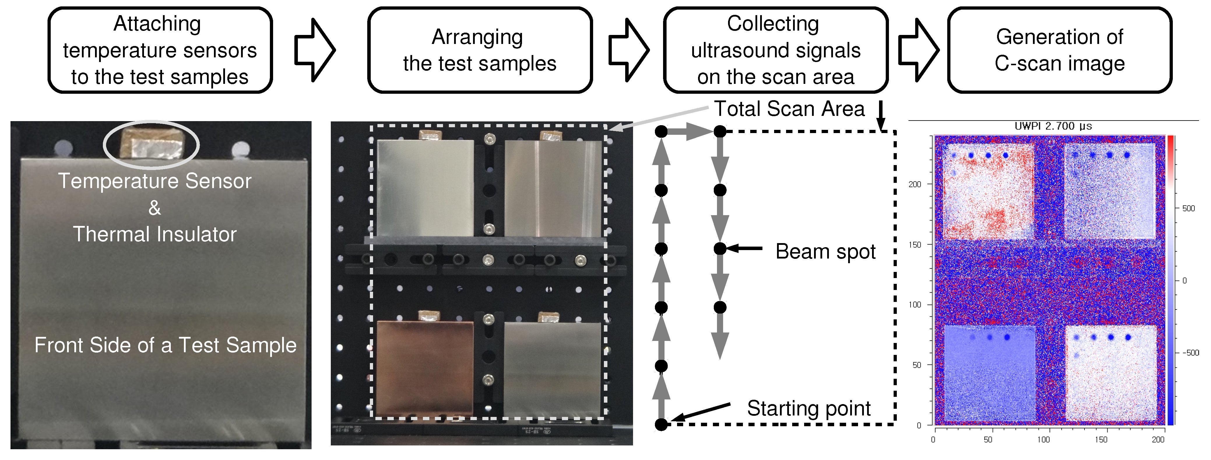
2. Experimental
2.1. Laser FF PE UPI System
2.2. Metal Plate Specimens
3. Results and Analysis
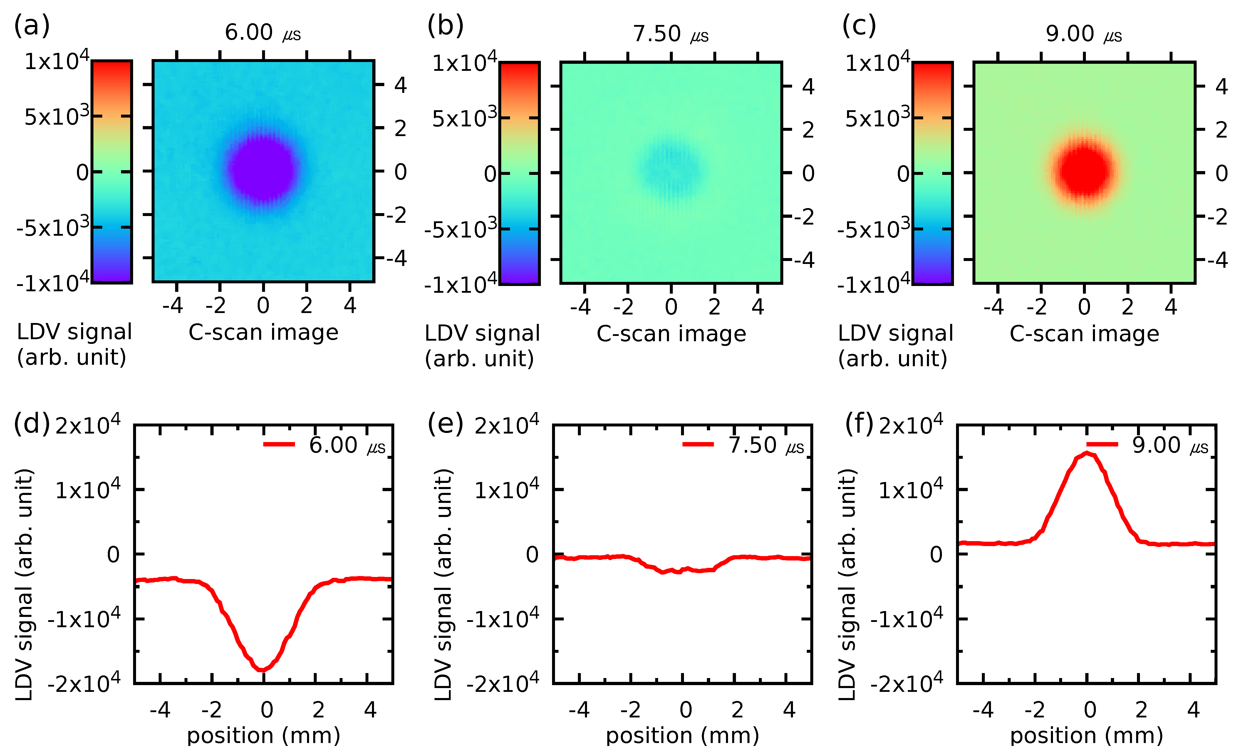
3.1. Characteristics of the Pulse-Echo Laser Ultrasonic Technique
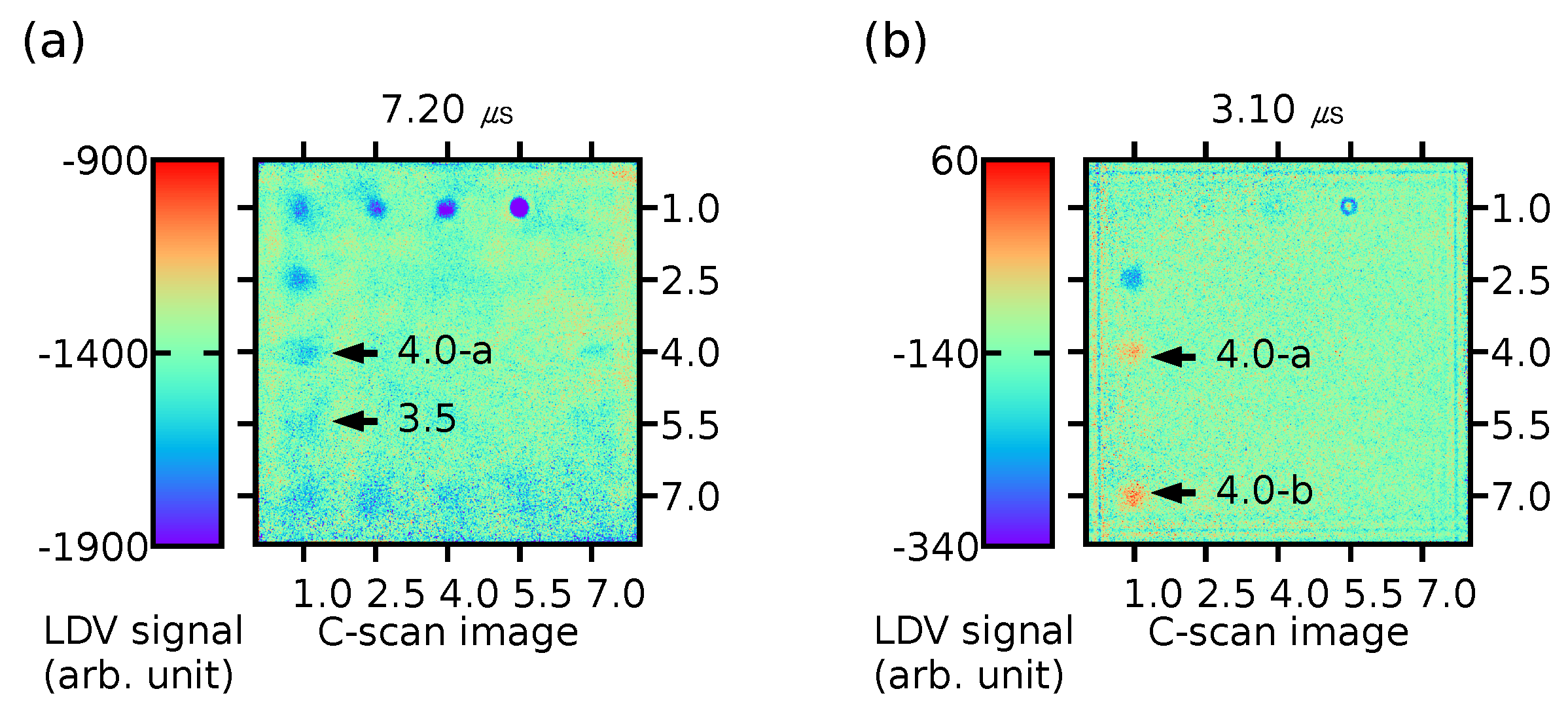
3.2. Criterion for the Detected Defects
3.3. Detected Artificial Defects
4. Discussion
5. Conclusions
Author Contributions
Funding
Institutional Review Board Statement
Informed Consent Statement
Data Availability Statement
Acknowledgments
Conflicts of Interest
References
- Jhang, K.Y. Nonlinear ultrasonic techniques for non-destructive assessment of micro damage in material: A Review. Int. J. Precis. Eng. Manuf. 2009. [Google Scholar] [CrossRef]
- Kwak, N.S.; Kim, J.Y.; Gao, J.C.; Park, D.K. Reliability Evaluation of Aircraft Brake Disk using the Non-contact Air-coupled Ultrasonic Transducer Method. J. Korean Soc. Manuf. Process Eng. 2016, 15, 36–43. [Google Scholar] [CrossRef]
- Lee, J.; Sheen, B.; Cho, Y. Quantitative tomographic visualization for irregular shape defects by guided wave long range inspection. Int. J. Precis. Eng. Manuf. 2015, 16, 1949–1954. [Google Scholar] [CrossRef]
- Miao, X.; Li, X.; Hu, H.; Gao, G.; Zhang, S. Effects of the oxide coating thickness on the small flaw sizing using an ultrasonic test technique. Coatings 2018, 8, 69. [Google Scholar] [CrossRef] [Green Version]
- Caenen, A.; Pernot, M.; Ekroll, I.K.; Shcherbakova, D.; Mertens, L.; Swillens, A.; Segers, P. Effect of ultrafast imaging on shear wave visualization and characterization: An experimental and computational study in a pediatric ventricular model. Appl. Sci. 2017, 7, 840. [Google Scholar] [CrossRef] [Green Version]
- Costa, P.; Nwawe, R.; Soares, H.; Reis, L.; Freitas, M.; Chen, Y.; Montalvão, D. Review of multiaxial testing for very high cycle fatigue: From ’Conventional’ to ultrasonic machines. Machines 2020, 8, 25. [Google Scholar] [CrossRef]
- Tanaka, T.; Izawa, Y. Nondestructive Detection of Small Internal Defects in Carbon Steel by Laser Ultrasonics. Jpn. J. Appl. Phys. 2001, 40, 1477–1481. [Google Scholar] [CrossRef]
- Kim, J.; Jhang, K.Y. Non-contact measurement of elastic modulus by using laser ultrasound. Int. J. Precis. Eng. Manuf. 2015, 16, 905–909. [Google Scholar] [CrossRef]
- Seo, H.; Kim, J.G.; Yoon, S.; Jhang, K.Y. Determination of laser beam intensity to maximize amplitude of ultrasound generated in ablation regime via monitoring plasma-induced air-borne sound. Int. J. Precis. Eng. Manuf. 2015, 16, 2641–2645. [Google Scholar] [CrossRef]
- Scruby, C.B.; Dewhurst, R.J.; Hutchins, D.A.; Palmer, S.B. Quantitative studies of thermally generated elastic waves in laser-irradiated metals. J. Appl. Phys. 1980, 51, 6210–6216. [Google Scholar] [CrossRef]
- Rothberg, S.J.; Allen, M.S.; Castellini, P.; Maio, D.D.; Dirckx, J.J.J.; Ewins, D.J.; Halkon, B.J.; Muyshondt, P.; Paone, N.; Ryan, T.; et al. An international review of laser Doppler vibrometry: Making light work of vibration measurement. Opt. Lasers Eng. 2017, 99, 11–22. [Google Scholar] [CrossRef] [Green Version]
- Hong, S.C.; Abetew, A.D.; Lee, J.R.; Ihn, J.B. Three dimensional evaluation of aluminum plates with wall-thinning by full-field pulse-echo laser ultrasound. Opt. Lasers Eng. 2017, 99, 58–65. [Google Scholar] [CrossRef]
- Shin, H.J.; Park, J.Y.; Hong, S.C.; Lee, J.R. In situ non-destructive evaluation of an aircraft UHF antenna radome based on pulse-echo ultrasonic propagation imaging. Compos. Struct. 2017, 160, 16–22. [Google Scholar] [CrossRef]
- Abetew, A.D.; Hong, S.C.; Lee, J.R.; Baek, S.; Ihn, J.B. Remote defect visualization of standard composite coupons using a mobile pulse-echo ultrasonic propagation imager. Adv. Compos. Mater. 2017, 26, 15–27. [Google Scholar] [CrossRef]
- Copper and Copper Alloy Sheets, Plates and Strips. KS D 5201. 2014.
- C12200 DHP Copper. Available online: http://ameritube.net/PDF/12200.pdf (accessed on 15 October 2019).
- Accoustic Properties for Metals in Solid Form. Available online: https://www.nde-ed.org/GeneralResources/MaterialProperties/UT/ut_matlprop_metals.htm (accessed on 15 October 2019).
- Rolled Steels for General Structure. JIS G 3101. 2004.
- Murakami, K.; Takemoto, M. Precursor of hydroigen induced glass lining chipping by AE monitoring. J. Acoust. Emiss. 2005, 23, 215–223. [Google Scholar]
- Callister William, D.J. Materials Science and Engineering: An Introduction, 6th ed.; WILEY: Hoboken, NJ, USA, 2002. [Google Scholar]
- Stella, J.; Cerezo, J.; Rodríguez, E. Characterization of the sensitization degree in the AISI 304 stainless steel using spectral analysis and conventional ultrasonic techniques. NDT E Int. 2009, 42, 267–274. [Google Scholar] [CrossRef]
- Lee, J.R.; Chia, C.C.; Park, C.Y.; Jeong, H. Laser ultrasonic anomalous wave propagation imaging method with adjacent wave subtraction: Algorithm. Opt. Laser Technol. 2012, 44. [Google Scholar] [CrossRef]


| Designed | Depth | 1.0 | 1.5 | 2.0 | 2.5 | 3.0 | 4.0 | 3.5 | 4.0 | 4.5 |
|---|---|---|---|---|---|---|---|---|---|---|
| Position | (55, 10) | (40, 10) | (25, 10) | (10, 10) | (10, 25) | (10, 40) | (10, 55) | (10, 70) | (25, 70) | |
| Copper alloy | 0.94 | 1.45 | 1.96 | 2.46 | 2.96 | 3.97 | 3.46 | 3.95 | 4.45 | |
| Stainless steel | 1.04 | 1.54 | 2.03 | 2.52 | 3.01 | 4.00 | 3.49 | 3.99 | 4.48 | |
| Hot rolled steel | 0.97 | 1.47 | 1.98 | 2.49 | 2.98 | 3.99 | 3.50 | 4.03 | 4.50 | |
| Aluminum alloy | 0.92 | 1.41 | 1.91 | 2.40 | 2.90 | 3.89 | 3.38 | 3.88 | 4.39 | |
| Defect-1.0 | Defect-1.5 | Defect-2.0 | Defect-2.5 | Defect-3.0 | Defect-4.0-a | Defect-3.5 | Defect-4.0-b | Defect-4.5 | ||
|---|---|---|---|---|---|---|---|---|---|---|
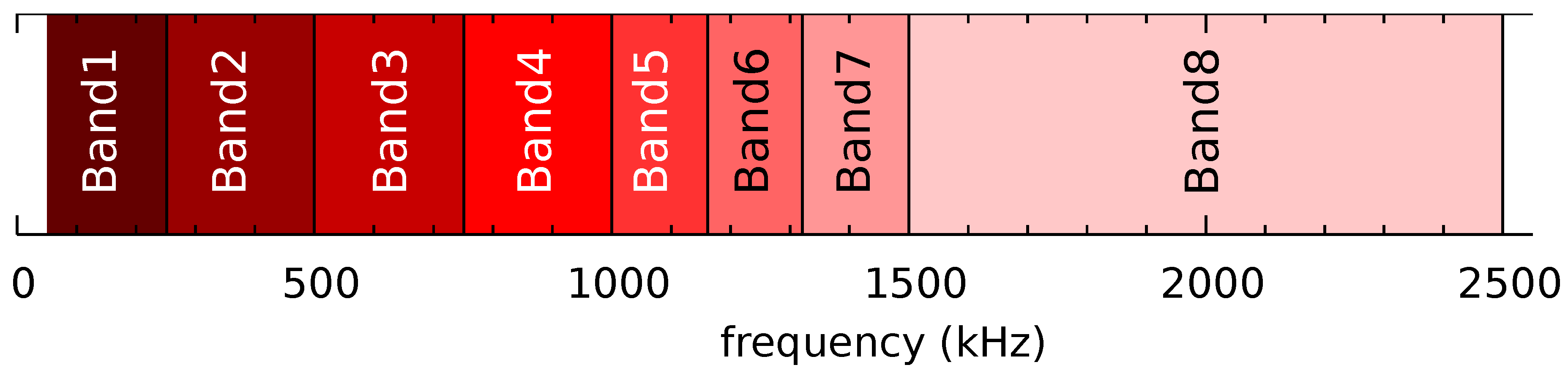
| Copper alloy | Band1 | ◯ | ◯ | ◯ | ◯ | ◯ | ||||
| (C1220) | Band2 | ◯ | ◯ | ◯ | ◯ | |||||
| Band3 | ◯ | ◯ | ◯ | ◯ | ||||||
| Band4 | ◯ | ◯ | ◯ | ◯ | ||||||
| Band5 | ◯ | ◯ | ◯ | |||||||
| Band6 | ◯ | ◯ | ◯ | |||||||
| Band7 | ◯ | ◯ | ◯ | |||||||
| Band8 | ◯ | |||||||||
| Stainless steel | Band1 | ◯ | ◯ | ◯ | ◯ | ◯ | ◯ | |||
| (STS304) | Band2 | ◯ | ◯ | ◯ | ◯ | ◯ | ◯ | ◯ | ||
| Band3 | ◯ | ◯ | ◯ | ◯ | ◯ | ◯ | ◯ | |||
| Band4 | ◯ | ◯ | ◯ | ◯ | ◯ | ◯ | ◯ | |||
| Band5 | ◯ | ◯ | ◯ | ◯ | ◯ | ◯ | ||||
| Band6 | ◯ | ◯ | ◯ | ◯ | ◯ | |||||
| Band7 | ◯ | ◯ | ◯ | ◯ | ◯ | |||||
| Band8 | ◯ | ◯ | ◯ | ◯ | ||||||
| Hot rolled steel | Band1 | ◯ | ◯ | ◯ | ||||||
| (SS400) | Band2 | ◯ | ◯ | ◯ | ||||||
| Band3 | ◯ | ◯ | ◯ | |||||||
| Band4 | ◯ | ◯ | ◯ | |||||||
| Band5 | ◯ | ◯ | ◯ | |||||||
| Band6 | ◯ | ◯ | ◯ | |||||||
| Band7 | ◯ | ◯ | ◯ | |||||||
| Band8 | ◯ | ◯ | ||||||||
| Aluminum alloy | Band1 | ◯ | ◯ | ◯ | ◯ | ◯ | ◯ | |||
| (AL6061) | Band2 | ◯ | ◯ | ◯ | ◯ | ◯ | ◯ | ◯ | ◯ | |
| Band3 | ◯ | ◯ | ◯ | ◯ | ◯ | ◯ | ◯ | ◯ | ◯ | |
| Band4 | ◯ | ◯ | ◯ | ◯ | ◯ | ◯ | ◯ | ◯ | ◯ | |
| Band5 | ◯ | ◯ | ◯ | ◯ | ◯ | ◯ | ◯ | |||
| Band6 | ◯ | ◯ | ◯ | ◯ | ◯ | ◯ | ||||
| Band7 | ◯ | ◯ | ◯ | ◯ | ◯ | |||||
| Band8 | ◯ | ◯ | ◯ |
Publisher’s Note: MDPI stays neutral with regard to jurisdictional claims in published maps and institutional affiliations. |
© 2021 by the authors. Licensee MDPI, Basel, Switzerland. This article is an open access article distributed under the terms and conditions of the Creative Commons Attribution (CC BY) license (https://creativecommons.org/licenses/by/4.0/).
Share and Cite
Kim, D.-I.; Jung, K.-R.; Jung, Y.-S.; Kim, J.-Y. Detectable Depth of Copper, Steel, and Aluminum Alloy Plates with Pulse-Echo Laser Ultrasonic Propagation Imaging System. Metals 2021, 11, 1607. https://doi.org/10.3390/met11101607
Kim D-I, Jung K-R, Jung Y-S, Kim J-Y. Detectable Depth of Copper, Steel, and Aluminum Alloy Plates with Pulse-Echo Laser Ultrasonic Propagation Imaging System. Metals. 2021; 11(10):1607. https://doi.org/10.3390/met11101607
Chicago/Turabian StyleKim, Dong-Il, Ku-Rak Jung, Yoon-Soo Jung, and Jae-Yeol Kim. 2021. "Detectable Depth of Copper, Steel, and Aluminum Alloy Plates with Pulse-Echo Laser Ultrasonic Propagation Imaging System" Metals 11, no. 10: 1607. https://doi.org/10.3390/met11101607
APA StyleKim, D.-I., Jung, K.-R., Jung, Y.-S., & Kim, J.-Y. (2021). Detectable Depth of Copper, Steel, and Aluminum Alloy Plates with Pulse-Echo Laser Ultrasonic Propagation Imaging System. Metals, 11(10), 1607. https://doi.org/10.3390/met11101607