Computational Determination of Macroscopic Mechanical and Thermal Material Properties for Different Morphological Variants of Cast Iron

Abstract

The sensitivity of macroscopic mechanical and thermal properties of grey cast iron is computationally investigated for a variety of graphite morphologies over a wide temperature range. In order to represent common graphite morphologies according to EN ISO 945-1, a synthetic approach is used to algorithmically generate simulation domains. The developed mechanical and thermal model is applied in a large simulation study. The study includes statistical volume elements of the graphite morphology classes GJL-150 and IA2 to IA5, with 10, 11 and 12  $\mathrm{v}.-\%$ of graphite precipitations, respectively, for a temperature range from 20 to 750 °C. Homogenised macroscopic quantities, such as the Young’s moduli, Poisson’s ratios, yield strengths and thermal conductivities, are predicted for different morphology classes by applying simulation and data analysis tools of the research data infrastructure Kadi4Mat. This is the first work to determine the mechanical and thermal properties of the morphology classes defined in EN ISO 945-1.

1. Introduction

Cast iron with lamellar graphite can be considered as a kind of natural composite material, consisting of a metallic matrix with embedded graphite particles [1,2,3,4]. To a large extent, both the mechanical and thermal properties of grey cast iron depend on the graphite morphology [5]. In this context, the shape, size, arrangement and volume fraction of graphite particles are referred to as graphite morphology. Depending on the individual casting practices of the foundries, the graphite morphology of a component, with nominally the same chemical composition, can differ from one foundry to the next [6]. Even with a constant volume fraction of graphite particles, large differences in material properties do occur, depending on the shapes, sizes and arrangements of the graphite particles [7,8,9]. In order to be able to specifically influence the casting process of a component in such a way that its thermomechanical properties are optimal, knowledge of the correlation between the morphology and the macroscopic properties is necessary. Against this background, continuum mechanical models are developed and are applied with the aid of numerical methods, so as to analyse the sensitivity of the macroscopic mechanical properties of cast iron with lamellar graphite independent of the graphite morphology over a wide temperature range. In the same manner, the influence of the graphite morphology on the thermal properties is investigated.

Particularly in the case of mechanical modelling, some aspects must be taken into account. In terms of the mechanical properties, cast iron with lamellar graphite has a complicated constitutive behaviour. Grey cast iron is tension–compression stress–strain asymmetric, which means that it shows non-linear elastic behaviour under a one-dimensional tensile load, and fails quasi-brittle, without pronounced macroscopic plastic deformation. Under a one-dimensional compressive load, it exhibits ductile behaviour and fails at much higher strains [10,11]. The asymmetry is also expressed in load-dependent Young’s modulus and yield strengths [10,11]. There is widespread consensus in the literature that tension–compression stress–strain asymmetric behaviour is a consequence of graphite lamellae and resulting interactions with the ductile matrix [11,12,13,14]. Under tensile load, graphite lamellae act as microcracks even at very small macroscopic strains and transmit almost no forces [6,12]. Due to this process, inhomogeneous mechanical fields arise in cast iron [10,12]. Stress peaks occur mainly at the sharp ends of graphite lamellae. At a macroscopic load far below the yield strength of the pure matrix material, local plastic deformations of the matrix occur due to the high stress concentrations [12]. Under pressure, the lamellae are pressed together and can thus transmit forces [6,12]; a larger force-transmitting volume exists. This results in more homogeneous mechanical fields [14,15]. The mechanical behaviour then resembles that of steel. From this load dependency, a tension–compression stress–strain asymmetry and bimodality arises. In Haenny and Zambelli [12], it is also assumed that due to the a strong difference in thermal expansions of graphite and the matrix, high eigenstrains develop during solidification, which lead to debonding. This theory is supported by Bonora and Ruggiero [1], as the matrix has a coefficient of thermal expansion that is at least one order of magnitude higher than that of graphite.

There are some publications which are also focused on the the correlation of the macroscopic properties of cast iron and its morphology. In the published works, the simulation domains were usually modelled using periodic unit cell approaches or by applying digitalised versions of real material samples. The obvious advantage of simulation domains created from real material samples is that they accurately represent the reality and cause the lowest possible uncertainty factor with regard to the simulation domain. In addition to the technologically complex creation of simulation domains, based on real material samples, it is not possible to specifically influence the morphology of the graphite. Thus, investigating the influence of these parameters on the macroscopic material properties is only feasible with extremely high effort. On the other hand, with the strongly idealised unit cell approaches, the transferability of the simulation results to reality is again difficult, since important characteristics of the graphite morphology, such as the cross-linking of the graphite lamellae, are not mapped quantitatively.

As an overview of the most important literature that deals with a similar problem to this publication, the following articles should be mentioned: Bonora and Ruggiero [1], Velichko et al. [3], Metzger and Seifert [14] and Pina et al. [16], Pina et al. [4] and Norman and Calmunger [11].

Bonora and Ruggiero [1] addresses the micromechanical behaviour of ferritic cast iron with spheroidal graphite. Special attention was paid to residual stresses that arose during cooling from melting to room temperature. Such residual stresses resulted from different coefficients of thermal expansion between the matrix of the cast iron material and the spheroidal graphite. For the simulations, periodic axisymmetric 2D unit cell simulation domains were used. The constitutive micromechanical model of the matrix corresponded to the elastoplastic von Mises behaviour, while the model of the spheroidal graphite represented linear–elastic material behaviour. Based on a Weibull probability distribution, which depends on the stress state, a method was used to describe the cracking behaviour of spheroidal graphite. Furthermore, matrix–graphite debonding was imitated, and ductile failure of the matrix was implemented using a continuum damage model.

Cast iron with lamellar graphite shows the best thermal and worst electrical conductivity of all cast iron variants, while cast iron with spheroidal graphite has values similar to steel and the values of cast iron with vermicular graphite lie between the two previously mentioned cast iron types. Against this background, Velichko et al. [3] tried to work out a correlation of these properties, with quantitative morphology characteristics. Among other things, FIB tomography images were used to create simulation domains, which were applied by means of an FEM analysis, in order to determine the electrical conductivity of cast iron with different graphite shapes. The tomography-based simulation domains represented geometrically accurate replicas of a small part of a real cast iron morphology, which resulted in the reproduction of experimental results. It was concluded that with computational modelling, one should be able to optimise morphologies to produce tailored composites that have maximised specific physical properties. It has also been shown that graphite cross-linking is a determining factor of the macroscopic material properties of cast iron.

Under cyclic mechanical load, cast iron with lamellar, vermicular and spheroidal graphite was examined by Norman and Calmunger [11]. The macroscopic material behaviour was calculated on the basis of a set of unit cell models, where each unit cell included a single randomly oriented graphite particle. All graphite lamellae had the shape of a penny-shaped ellipsoid and showed purely elastic, transversely isotropic material behaviour. To model the cyclic load appropriately, the matrix behaved like a plastic–isotropic medium with a von Mises flow behaviour and kinematic hardening.

To study the thermal and mechanical properties of cast iron with lamellar graphite, a periodic unit cell model was used by Pina et al. [16], which considered the cross-linking of the graphite particles. The graphite particle of a unit cell had a complex three-dimensional “star shape”, which captured the most important morphological features of real morphology in an idealised way. The matrix was regarded as a homogeneous, isotropic–elastoplastic material, while the graphite was treated as a linear–elastic material with a transverse isotropy.

Metzger and Seifert [14] used statistical volume elements of realistic cast irons with lamellar graphite morphologies as a simulation domain, which were generated using the serial sectioning method. The isotropic graphite had a Young’s modulus that depended on the strain state. The matrix possessed plastic von Mises behaviour, with the parameters of the plastic model adjusted in such a way that the numerical stress–strain curves of the morphology-based model fitted well with experimental compression tests.

In contrast to the previously published approaches, the present work uses “synthetic methods” to generate complex morphologies. Here, the shape, the spatial expansion and the arrangement of the graphite lamellae, including their cross-linking, are reproduced realistically, whereby the expression of these characteristics can be influenced as desired and the volume fraction of the graphite particles can also be freely defined. In a large temperature range, this approach allows quantitative statements to be made about the influence of different spatial morphology of the graphite lamellae and different graphite volume fractions on macroscopic mechanical and thermal material properties. All possible manifestations of the graphite morphology are given by statistical volume elements (SVEs). As already predicted by Velichko et al. [3], the obtained data can be used to design customised morphologies with maximised physical properties in order to adjust the casting process and/or the alloy components of a material in such a way that a solidified component has a desired morphology.

For the temperature range from 20 to 750 °C, the database, created by means of the conducted simulation study, includes the following macroscopic mechanical and thermal properties: Young’s modulus, Poisson’s ratio and the respective yield strength under tensile and compressive load, as well as the thermal conductivity. All properties are investigated by means of the specified shape and arrangement of the graphite particles, varying the size distribution of the graphite lamellae and the volume fraction of the graphite inclusions. The material parameters of the microscopic models depend on the temperature $\theta$.

The EN ISO 945-1 [17] standard allows the graphite morphology in a cast iron casting to be classified by visual evaluation, based on the shape, the arrangement and the size of the graphite. The standard is used to define the possible variants of graphite morphologies, whereby the simulation study only includes a part of the variants contained in the EN ISO 945-1 standard, simply to reduce the amount of work. In the study, graphite of type IA2 to IA5 and a purely pearlitic matrix are considered. The graphite particles of the graphite lamellae thus have a spatial expansion from $0.06$ to $1.0$ $\mathrm{m}$$\mathrm{m}$.

Table 1. Guide numbers of size ranges, according to the EN ISO 945-1 standard.

Guide Number	Value	Unit
IA2	$0.5$ to $<1.0$	$\mathrm{m}\mathrm{m}$
IA3	$0.25$ to $<0.5$	$\mathrm{m}\mathrm{m}$
IA4	$0.12$ to $<0.25$	$\mathrm{m}\mathrm{m}$
IA5	$0.06$ to $<0.12$	$\mathrm{m}\mathrm{m}$

lists the spatial dimensions of the various classes 2 to 5, according to the EN ISO 945-1 standard.

The limitation of the simulation study is not a restriction of the methodology, i.e., the described procedure can also be applied to cast iron variants with other graphite forms, for example, vermicular graphite, or ferritic matrix material. However, this requires an adaptation of the shape definition and the distribution functions of the graphite particles for the creation of simulation domains.

The creation of a database that maps the relationship between graphite morphology and macroscopic mechanical and thermal properties of cast iron with lamellar graphite can also be carried out via a large number of experiments, i.e., entirely without numerical methods. Such an approach would require a non-destructive detection of the morphology, for example, before tensile tests are carried out, using the focused ion beam method [18] or microtomography [19]. Since the morphology actually present in a material is unknown in advance, it is very likely that a far greater number of material samples must be experimentally examined, compared with the number of possible different variants of the morphology, to obtain the complete range of different morphologies. Combined with the large temperature range for which the macroscopic mechanical and thermal properties are to be acquired an enormous number of expensive and time-consuming experiments would thus be necessary to create the desired database. Furthermore, hypothetical morphologies can only be investigated using a digital approach. In the present work, therefore, digital methods are chosen in preference to an experimental approach. Once the numerical framework for a digital determination of morphology-dependent, macroscopic mechanical and thermal properties is developed, the methodology can be transferred to other materials with comparatively little effort and cost, which in turn supports the development of such a framework.

In the following Section 2, the methodology used to create the simulation domains is explained. Subsequently, the microscopic material models, together with the required material parameters, are introduced (Section 3), distinguishing between the models for the pearlitic matrix (Section 3.1) and the lamellar graphite (Section 3.2). This is followed by mechanical simulations (Section 4), including the key points of the numerics and the simulation setup (Section 4.1) and a model analysis of the mechanical model (Section 4.2). Afterwards, the results of the simulation study are presented in Section 4.3. The results of the thermal simulations are given in Section 5. An overview of the correlations between the morphology-dependent thermal and mechanical properties is given in Section 6. Finally, an overview of the results and possible further work is given in Section 7.

2. Creating Simulation Domains for Cast Iron with Lamellar Graphite

Applying morphology generation, simulation and characterisation methods of the research data infrastructure Kadi4Mat, the macroscopic mechanical material behaviour and the thermal conductivity of cast iron with lamellar graphite are investigated, due to changing graphite morphology. For this purpose, 3D simulation domains that depict the observed range of all possible morphologies with sufficient accuracy are necessary. The challenge in predicting cast iron properties based on graphite morphology is associated with the diversity of the size, shape and spatial arrangement of graphite inclusions [3]. In particular, with regard to the numerical determination of the thermal conductivity of cast iron, 2D simulation domains do not provide accurate results, as the cross-linking of graphite particles in 2D domains is not taken into account [3], which is why 3D simulation domains have to be used.

In general, simulation domains can be generated using two different methods. On the one hand, simulation domains can be generated directly on the basis of real existing material samples. In Chawla et al. [20] or Metzger and Seifert [14], for example, the 3D morphology of real material samples, consisting of an aluminium composite material reinforced with silicon carbide or grey cast iron, was reconstructed using the serial sectioning method. Serial sectioning involves generating a large number of micrographs of a material sample, removing very little material between each micrograph by polishing, which are then combined to form a 3D simulation domain. The focused ion beam method (FIB) and 3D microtomography are suitable as further methods of 3D morphology detection that do not destroy material samples. Velichko et al. [18] used the focused ion beam method to analyse the topology of lamellar, spherical and vermicular graphite in grey cast iron. The 3D morphology formed during dendritic solidification was studied by Limodin et al. [19] using microtomography. The methods mentioned here allow the digital representation of adequate 3D morphologies. For this purpose, however, special experimental equipment is required. In addition, the practical application is a great challenge. The costs of generating the necessary digital replicas using experimental methods would probably exceed the costs of the experimental identification of mechanical and thermal material properties, and are therefore not used.

Besides the generation based on real existing material samples, cast iron simulation domains can also be generated “synthetically”. The idea with synthetic simulation domains is that the complex material behaviour, resulting from the morphology, is reproduced, even though the geometric representation of the morphology does not correspond exactly to that of the real material. In the case of cast iron, this is achieved by simulation domains that have a similar statistical occurrence of inclusions compared to real materials [3]. Synthetic methods thus provide simplified and idealised morphologies, yet they must capture the main characteristics of a real morphology. It is therefore important to identify and consider all relevant properties of the morphology that have a significant influence on the mechanical and thermal behaviour of the material.

Compared to an experimental approach for creating simulation domains, some advantages of a synthetic approach are absolutely necessary for the simulation study in this work, whereby the range of the morphologies was initially determined by definition. The extent of the morphologies corresponds to the graphite classes IA2 to IA5. With regard to the volume fractions of the graphite flakes, we limit ourselves to 10, 11 and 12 $\mathrm{v}.-\%$. As a representative example for a cast iron material in practical application, GG-15 / GJL-150 is considered as a composition of the cast iron classes IA2 to IA5. The generation of morphologies corresponding to the graphite classes IA2 to IA5 is realised in a synthetic manner, as the size distribution of the graphite lamellae, given for a graphite class of EN ISO 945-1, does not occur in real castings, because a mixture of the different graphite characteristics is always present in reality. Characteristics such as the size distribution of the lamellae and the volume fraction of the graphite can only be influenced precisely when the domain is generated synthetically. During the synthetic creation of the simulation domains, the orientations of the anisotropies of the graphite inclusions can be saved. Thus, the transversal isotropy of the graphite lamellae can be taken into account, which is a challenge when using real morphologies. In general, it can be said that the generation of synthetic morphologies is associated with considerably less effort and can be carried out flexibly, compared to an experimental generation and in a tailored manner, but with the disadvantage of lower accuracy.

The approach that represents the greatest idealisation of synthetic domain generation is the unit cell approach. Here, the morphology of cast iron is replicated by simple identical and periodic unit cells. A unit cell contains a single graphite particle, embedded in matrix material. In the case of spheroidal graphite cast iron, this procedure reproduces the most important properties of a real graphite morphology. In the case of more complex morphologies, such as cast iron with lamellar graphite, important characteristics such as the cross-linking of the graphite are either not captured or it is difficult to draw analogies to real materials.

Before describing the developed method for synthetic domain generation, one terminology still needs to be clarified. Graphite lamellae have a much larger spatial extent within the basal planes due to their main growth direction along the a-direction of the hexagonal crystal lattice [21], compared to their extent orthogonal to the basal planes [22]. In the following, the directions of the larger spatial expansions (a-direction) of a graphite lamella are referred to as the longitudinal direction.

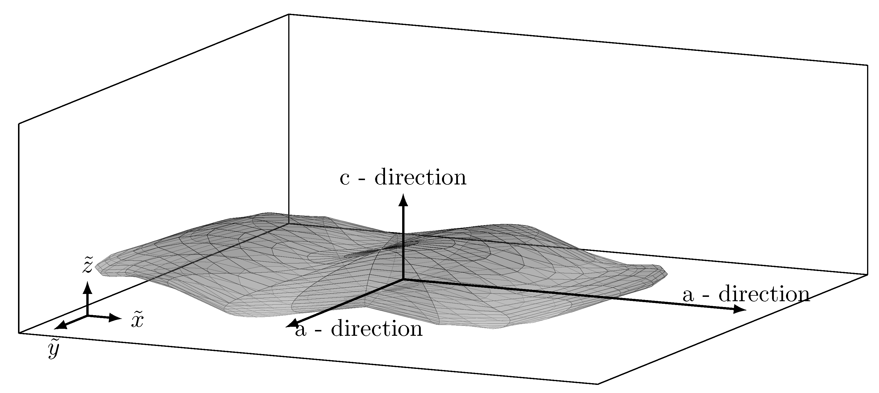
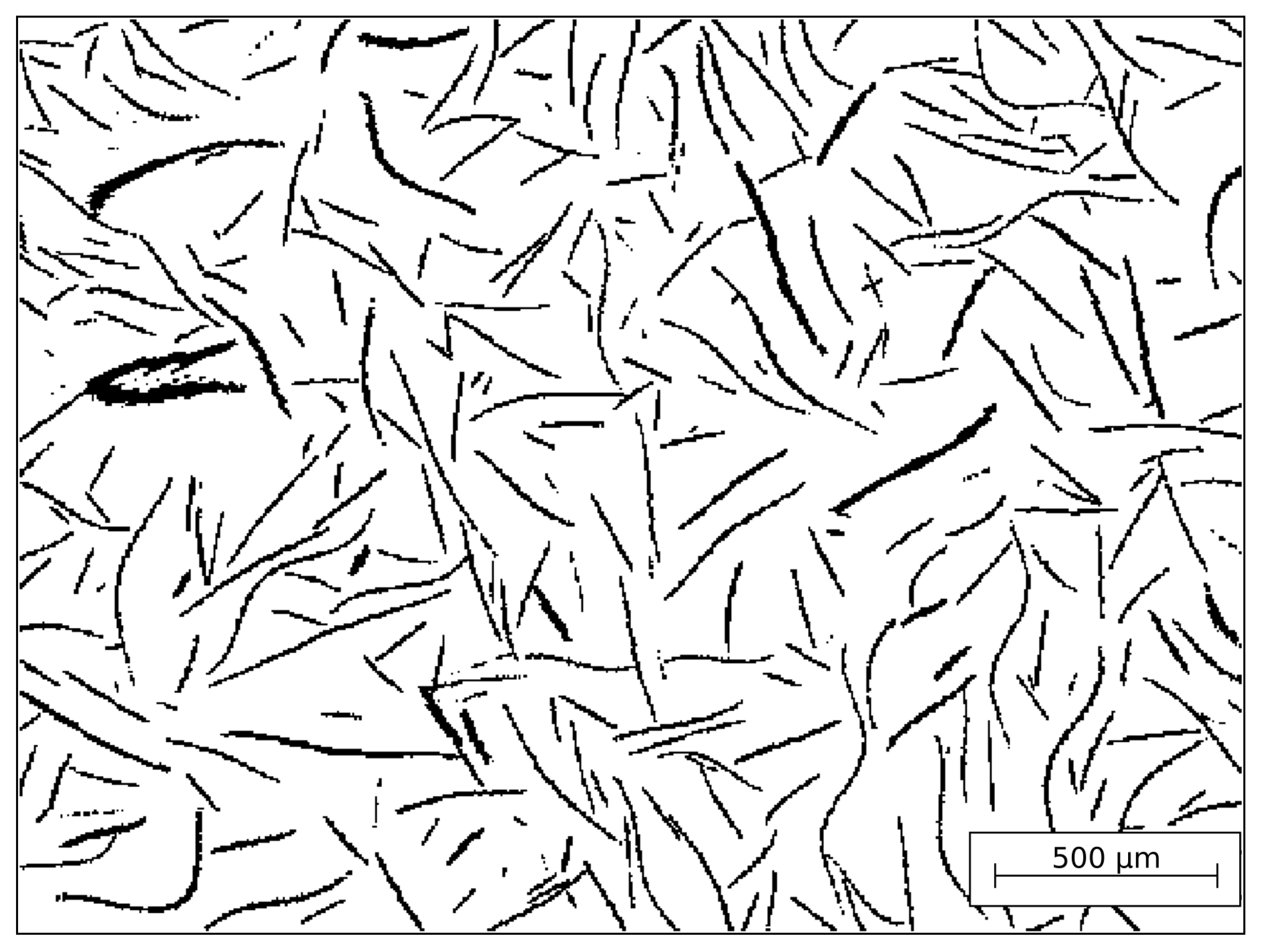
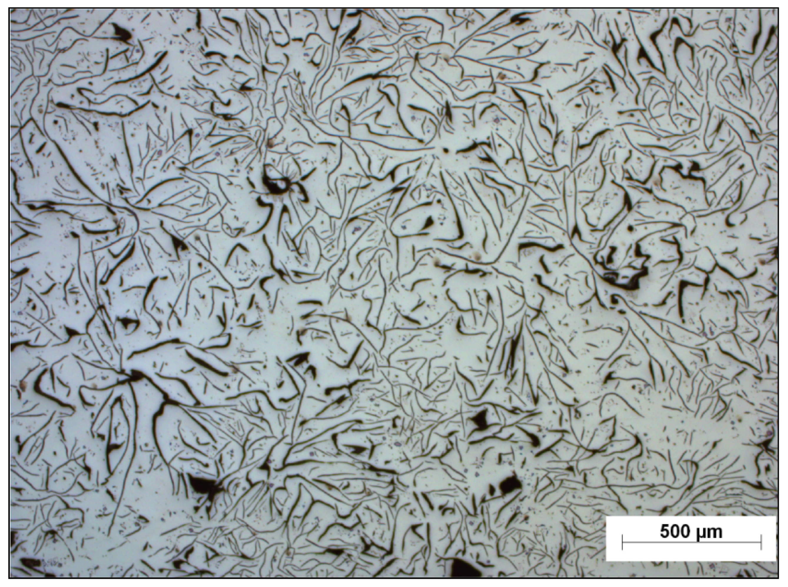
2.1. Modelling the Morphology of Cast Iron with Lamellar Graphite

In contrast to Pina et al. [16] and Norman and Calmunger [11], the developed methodology for morphology generation is not a unit cell model. Compared to the unit cell approaches, the use of complex morphologies offers the advantage of a better transferability of the synthetic graphite morphology to real morphologies. Certain idealising and simplifying assumptions are made regarding the shape, size, arrangement and distribution of the graphite lamellae. The shape of the inclusions of cast iron with lamellar graphite is often described as lamellar or flake-like [16], which is why the graphite lamellae are modelled as flat corrugated ellipsoids. In a particle-specific $\tilde{x},\tilde{y},\tilde{z}$ coordinate system, a single lamella is mathematically described by:

$$\begin{array}{c}\hfill \frac{{\tilde{x}}^2}{r^2}+\frac{{\tilde{y}}^2}{s^2}+\frac{{\left(\tilde{z}+amp\ast \sin (freq\ast \tilde{x}+offset)\right)}^2}{t^2}\le 1\end{array}$$

(1)

Here, $r,s$ and t are the semi-axes of the ellipsoid, and $amp,freq$ and $offset$ are the amplitude, the frequency and the zero phase angle of a corrugation of the ellipsoid along the $\tilde{x}$ axis. The longitudinal axes (a-direction) lie in the $\tilde{x}$-$\tilde{y}$ plane and the $\tilde{z}$ axis is parallel to the c-direction of the hexagonal crystal lattice, which results in $t\ll r,s$. In Figure 1, the schematic representation of a single graphite lamella is shown.

Knowing the orientation of the $\tilde{x},\tilde{y},\tilde{z}$ coordinate system, the orientation of the transversely isotropic material properties can be considered in a $x,y,z$ reference coordinate system. The idealised shape of the graphite lamellae is similar to that of the unit cell model according to Norman and Calmunger [11], with the extension of each lamella having a corrugation imposed on it. In Norman and Calmunger [11], a unit cell consists of an isolated, penny-shaped, ellipsoidal graphite particle, embedded in a homogeneous steel matrix. In contrast to the method developed in this work, no cross-linking between the graphite inclusions exists in the unit cell approach. In addition to the basic shape of the graphite particles, statistical distribution functions corresponding to those of real material samples must be defined for the following characteristics, in order to be able to define adequate morphologies: the positioning, the orientation (orientation of the c-axis of an ellipsoid in the $x,y,z$ reference coordinate system), the length (parameter r), the width (parameter s) and thickness (parameter t), as well as the amplitude (parameter $amp$), the frequency (parameter $freq$) and the zero phase angle (parameter $offset$) of the corrugations of the graphite lamellae. The choice of the position and rotation of the particles in the simulation domain, and furthermore, that of the zero phase angles, is randomly equally distributed. Additionally, the condition regarding the position of particles is fulfilled, so that no overlapping of particles occurs. By applying an equal distribution of the positioning and rotation, a deviation of the synthetic morphologies does occur, in comparison to a real morphology. The arrangement of graphite lamellae is often controlled by a growth mode of eutectic cells, as, e.g., discussed in Noguchi and Shimizu [23]. The presence of graphite lamellae in clusters is covered in terms of EN ISO 945-1 by the graphite class IB, which is by definition not considered in this work and might be the topic of future research. The length and width distribution of the particles, i.e., the dimensions of the longitudinal axes, are assumed to be subject to a normal distribution. The parameters of the normal distribution of the longitudinal axes of a given morphology class are selected according to the standard EN ISO 945-1 [17]. An IA2 morphology is used as an example to explain the choice of parameters. In an IA2 morphology, graphite lamellae of lengths or widths, $l^{IA2}$, of $0.5$ to $1.0\mathrm{m}\mathrm{m}$ occur. In this case, a mean value of ${\mu }^{IA2}=0.75\mathrm{m}\mathrm{m}$ is chosen for the normal distribution. This corresponds to the arithmetic mean of the minimum, $l_{\min }$, and maximum length or width, $l_{\max }$, of the particles of a graphite expression:

$$\begin{array}{c}\hfill \mu =\frac{l_{\min }+l_{\max }}{2}.\end{array}$$

(2)

The variance, $var$, is chosen in such a way that the minimum or maximum spatial extent corresponds to twice the standard deviation:

$$\begin{array}{c}\hfill var=\frac{l_{\min }+l_{\max }}{8}.\end{array}$$

(3)

At this point, it cannot be proven that the assumption of a normal distribution of the lengths and widths of graphite lamellae corresponds to reality, as no experimental investigation results of real 3D morphologies are available in this respect. In our estimation, however, the normal distribution is the most plausible probability distribution. The type of distribution functions and the corresponding parameters of the thickness, the amplitude and the frequency of the corrugation are determined by means of an improved version of the analysis tool presented in Schmid et al. [24], using micrographs from Schmid [25]. For the thickness and the frequency, this results in a normal distribution, while for the amplitude, this leads to a Chi-Square distribution. Here, it is assumed that the distribution functions determined on the basis of 2D micrographs can be transferred to 3D morphologies, which, however, is only partially the case with non-convex geometries.

The algorithm for synthetically generating 3D domains that mimic the morphology of cast iron with lamellar graphite can be summarised verbally as follows: during the generation of simulation domains of predefined sizes, graphite particles are gradually inserted into the domains. For each iteration step, the orientation, length, width, thickness as well as the amplitude, frequency and the zero phase angle of the corrugation of a new graphite lamella are determined by means of the applied probability distributions. Then, a position in the simulation domain is selected in such a way that there is no overlap between a new graphite lamella and the graphite particles already present in the simulation domain. Thus, if an overlap of two particles occurs at a certain position, a new position is selected randomly until no more overlap occurs. The avoidance of overlapping graphite particles causes new particles to be aligned parallel to their neighbours beyond a certain number of existing particles in the simulation domain. This automatically results in a lamellar arrangement of the graphite flakes. As soon as the desired graphite volume fraction is found in the simulation domain, the algorithm terminates.

The matrix of cast iron is assumed to be purely pearlitic. Pearlite is a heterogeneous material, consisting of many pearlite colonies. Each colony is composed of many alternating parallel, thin layers of ferrite and cementite. In the work of Langford [26], it was shown that the elastic properties of ferrite and cementite are almost identical. However, enormous differences exist with regard to plastic properties and strength. Due to the different plastic properties and strengths of ferrite and cementite, the lamellar structure of a single pearlite colony results in a generally anisotropic material behaviour. In the case of a uniaxial mechanical load, however, Peng et al. [27] demonstrated that the behaviour of a single pearlite colony is independent of whether it is loaded parallel or perpendicular to the alternating lamellar planes. This means that a single pearlite colony behaves isotropically under uniaxial mechanical loading. Since only mechanical simulations with macroscopic uniaxial loading are performed in the context of this work, the pearlitic matrix is idealised as homogeneous and isotropic, similar to the publications in [4,11,14,16]. Furthermore, the anisotropy of the thermal conductivity of pearlite colonies is neglected. This is justified by the fact that pearlite, compared to lamellar graphite, only has a negligible anisotropy of thermal conductivity. Thus, the simulation study only captures the influence of a changing graphite morphology on the macroscopic properties and not the influence of a changing morphology of the pearlite.

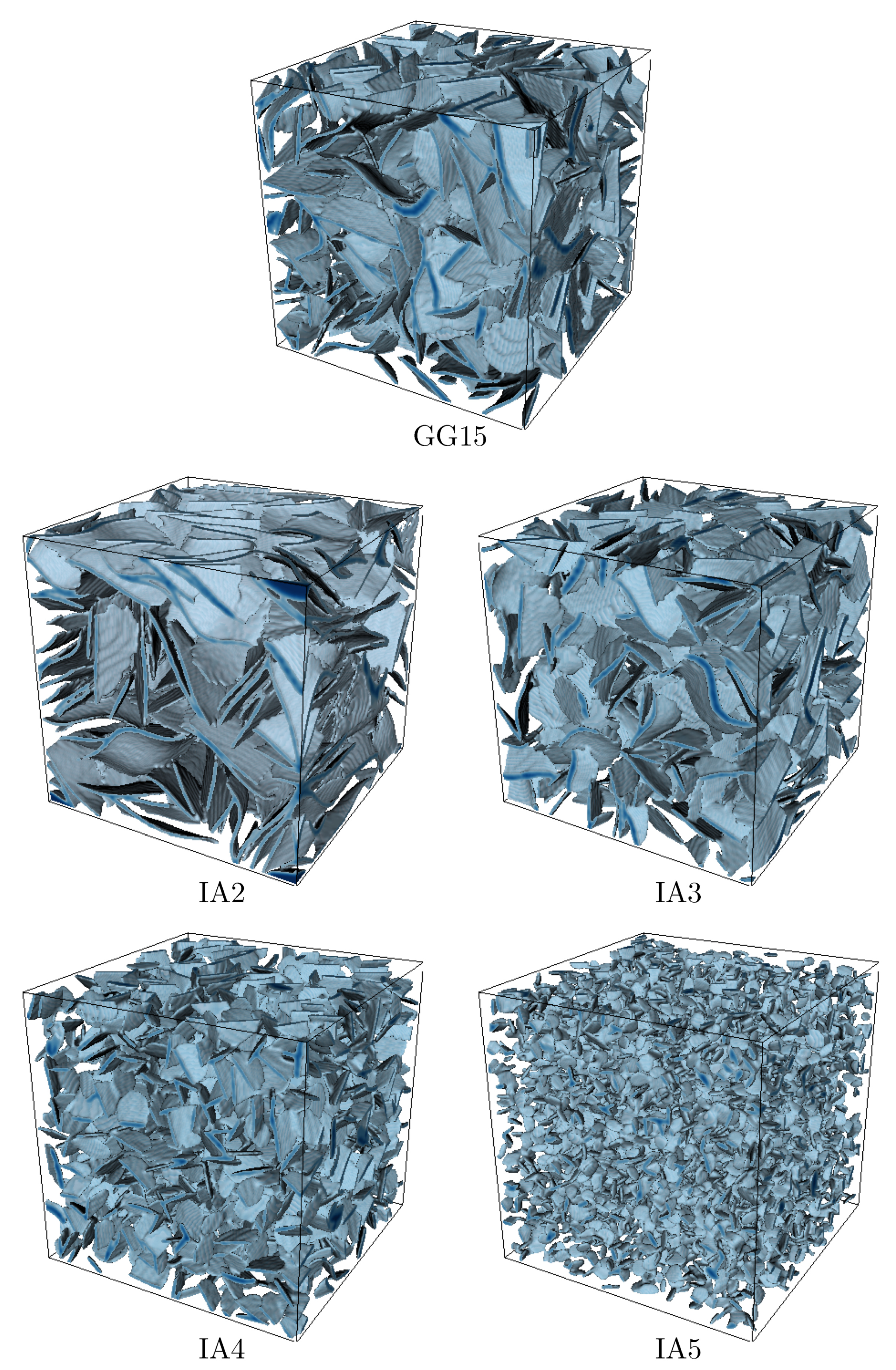
2.2. The Volume Elements

Ideally, the simulation domains used should correspond to so-called representative volume elements (RVEs). According to Hill [28], an RVE is understood to be “the smallest volume over which a measurement can be made that gives a value representative of the whole (heterogeneous material)”. In experimental macroscopic tests, cast iron with lamellar graphite behaves isotropically. A grey cast iron RVE would therefore have to contain a sufficiently large number of transversely isotropic graphite particles, so that their anisotropy, viewed macroscopically, is statistically eliminated. Due to the high number of graphite lamellae necessary to obtain macroscopic isotropic material behaviour, the simulation study cannot be performed on representative volume elements. Instead, statistical volume elements (SVEs) are used, as in Metzger and Seifert [14].

For graphite lamellae of class IA2, aspect ratios of up to $1/200$ can occur between the thickness and length of a particle [14]. This corresponds to a lamella thickness of $5\mathsf{\mu }\mathrm{m}$, with a length of $1000\mathsf{\mu }\mathrm{m}$. For numerical reasons, each graphite lamella must have a minimum height of three voxels, so that the curvature, which is caused due to the corrugation of the particles, is represented with sufficient accuracy. Thus, from the aspect ratio of $1/200$ of a graphite lamella and a minimum height of three voxels, a length of 600 voxels follows for a single particle, in the extreme case. Simulation domains of at least $600\Delta x\times 600\Delta y\times 600\Delta z$ voxels would be therefore necessary to be able to contain a single particle, which is not feasible with regard to the computational effort. In the generated simulation domains, the maximum aspect ratio of the graphite particles is restricted to $3/200$.

Figure 2 shows an example of a 2D section through a synthetically generated GG-15 material, with a graphite flake volume fraction of $10\mathrm{v}.-\%$. GG-15 is hereby the old designation of the GJL-150 material. Next to it in Figure 3, the micrograph of a specimen taken from a truck brake disc, made of GG-15 Cr Cu Nb HC [25], is shown. The two “micrographs” represent sections of the same physical size, $2730\mathsf{\mu }\mathrm{m}\times 2040\mathsf{\mu }\mathrm{m}$.

It can be observed that the synthetically generated and experimental micrographs are visually similar when neglecting the very small particles by looking at Figure 2 and Figure 3. To some degree, in addition, differences in micrographs may result to from cross-sectional preparation. The characteristic features of the graphite particles, such as lengths, thicknesses as well as the amplitudes and frequencies of the corrugations, are apparently well reproduced by the described method. A significant difference can only be seen with regard to the arrangement of the graphite particles. However, this difference can be explained by the fact that no eutectic cell of the type IB graphite is considered by the morphology creation algorithm applied. It should be noted that a similarity of the “micrographs” does not necessarily imply a similarity of the underlying 3D morphology. As soon as the shape of the graphite particles is not convex, the reconstruction of their 3D shape, with the help of a micrograph, is almost impossible for irregular and asymmetrical particles [18].

In Figure 4, spatial images of synthetically generated statistical volume elements of the graphite morphologies GJL-150 and IA2 to IA5 are shown, each with a graphite flake volume fraction of 10 $\mathrm{v}.-\%$. It clearly becomes evident that the number of graphite lamellae in the simulation domains increases from IA2 to IA5 for the same graphite volume fraction as the average size of the graphite particles decreases.

All volume elements shown here possess the same physical size of $1.25\mathrm{m}\mathrm{m}\times 1.25\mathrm{m}\mathrm{m}\times 1.25\mathrm{m}\mathrm{m}$. For the simulation study, statistical volume elements of this size are used. Each statistical volume element consists of $250\Delta x\times 250\Delta y\times 250\Delta z$ voxels, while a voxel has a physical size of $5\mathsf{\mu }\mathrm{m}\times 5\mathsf{\mu }\mathrm{m}\times 5\mathsf{\mu }\mathrm{m}$. An equidistant, orthogonal grid is used to spatially discretise the simulation domains. For the variation of the graphite characteristics, according to the EN ISO 945-1 classification, only the normal distribution of the lengths and widths is changed. All graphite morphologies obtain constant parameters of the probability distribution functions for graphite lamella thickness, amplitude and frequency. Thus, there is no self-similarity between the simulation domains, since, for example, the aspect ratio of the thickness and length changes. This is important, because different simulation results are only based on different morphologies and not on scale effects. For the quantitative comparison of morphologies, the ratio of the surface area of a particle to its volume is introduced as a parameter, ${\varphi }_i=A_i/V_i$. The arithmetic mean of the parameters, ${\varphi }_i$, over all particles of the simulation in the analysed domains results in: ${\varphi }^{GJL-150}=1.28\mathsf{\mu }\mathrm{m}$, ${\varphi }^{IA2}=1.24\mathsf{\mu }\mathrm{m}$, ${\varphi }^{IA3}=1.27\mathsf{\mu }\mathrm{m}$, ${\varphi }^{IA4}=1.32\mathsf{\mu }\mathrm{m}$ and ${\varphi }^{IA5}=1.42\mathsf{\mu }\mathrm{m}$. Here, the parameters of GJL-150 and IA3 are the most similar, which also suggests a similarity of their mechanical and thermal properties.

For simulation domains of the same graphite class, e.g., IA2, but with a different graphite volume fraction, the following procedure is used: each simulation domain of a graphite class contains exactly the same graphite particles as an SVE of the same graphite class with a lower volume fraction. A higher volume fraction is achieved by adding additional graphite lamellae to a volume element with a lower graphite volume fraction, until the desired larger graphite volume fraction is reached. This procedure is required as no representative volume elements are used. When investigating the influence of an increasing graphite volume fraction, it is thus guaranteed that changes of macroscopic material properties only result from different graphite volume fractions and not from a difference in the “base” morphology.

3. Model Formulation

In the following section, the applied microscopic mechanical and thermal models are introduced and the used material parameters are presented. A distinction is made between the models for the pearlitic matrix and those for the graphite lamellae. The assumptions made are based on Ockham’s philosophy: “The simplest solution is the best solution”. This means that several simplifying assumptions are made to make the complexity of the physical reality manageable and to ensure reasonable computational effort. Any assumption is justified by plausible reasons.

Small deformations are assumed, which means that only macroscopic strains up to $2\%$ should be considered in one-dimensional tensile and compression tests, in order to avoid significant kinematic errors. This critical value of the macroscopic strain is enforced in all performed simulations. Nevertheless, local regions with higher deformations can occur, which do not fulfil the mathematical requirements for the geometrical linearisation. This happens under tensile load at macroscopic strains $<2\%$, as some graphite lamellae act as microcracks, causing local stress and strain concentrations [12]. The neglect of the occurring geometric non-linearities is due to a minimisation of the computational costs and is justifiable, since large deformations only occur in a small region of the simulation domains.

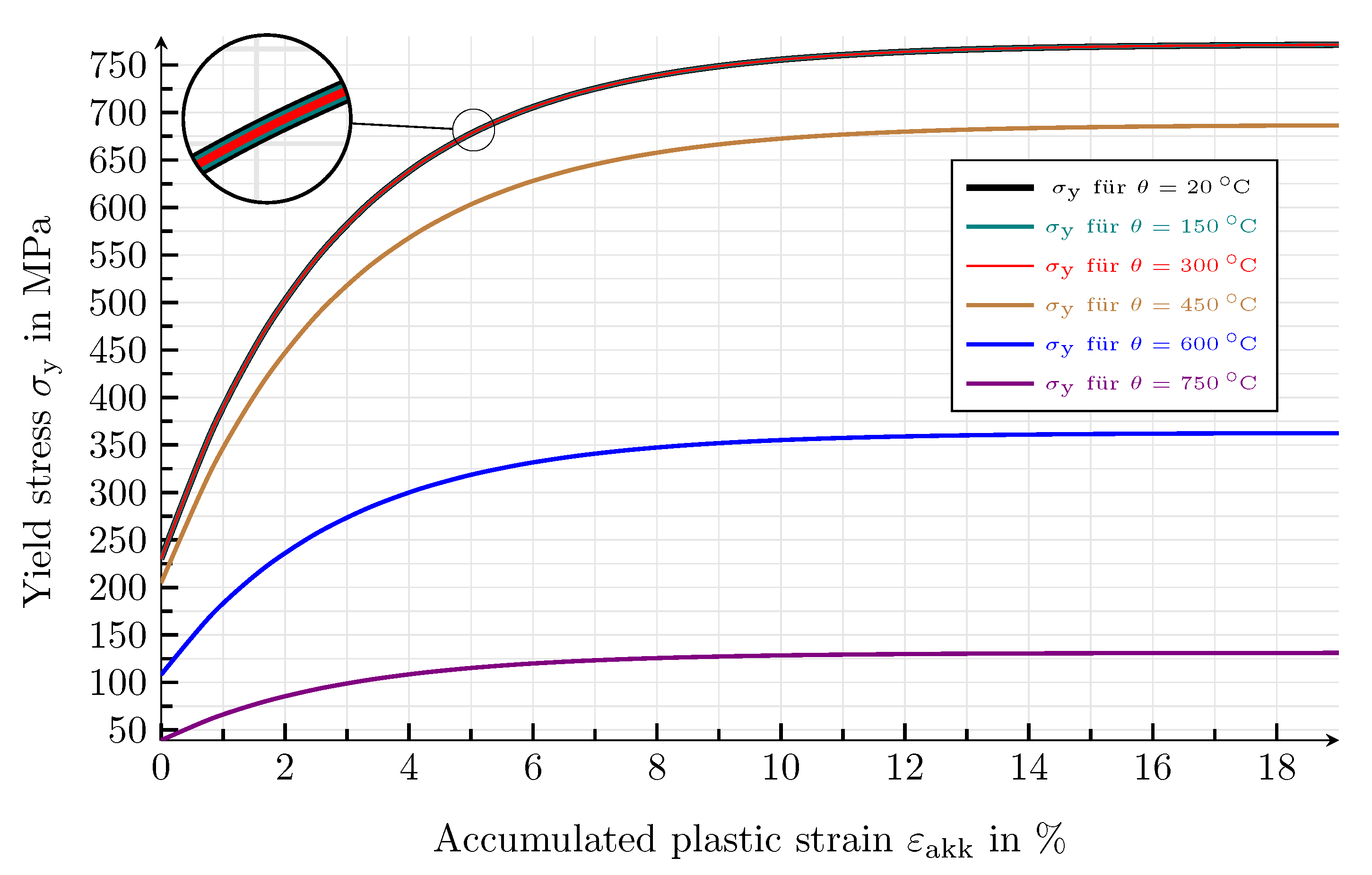
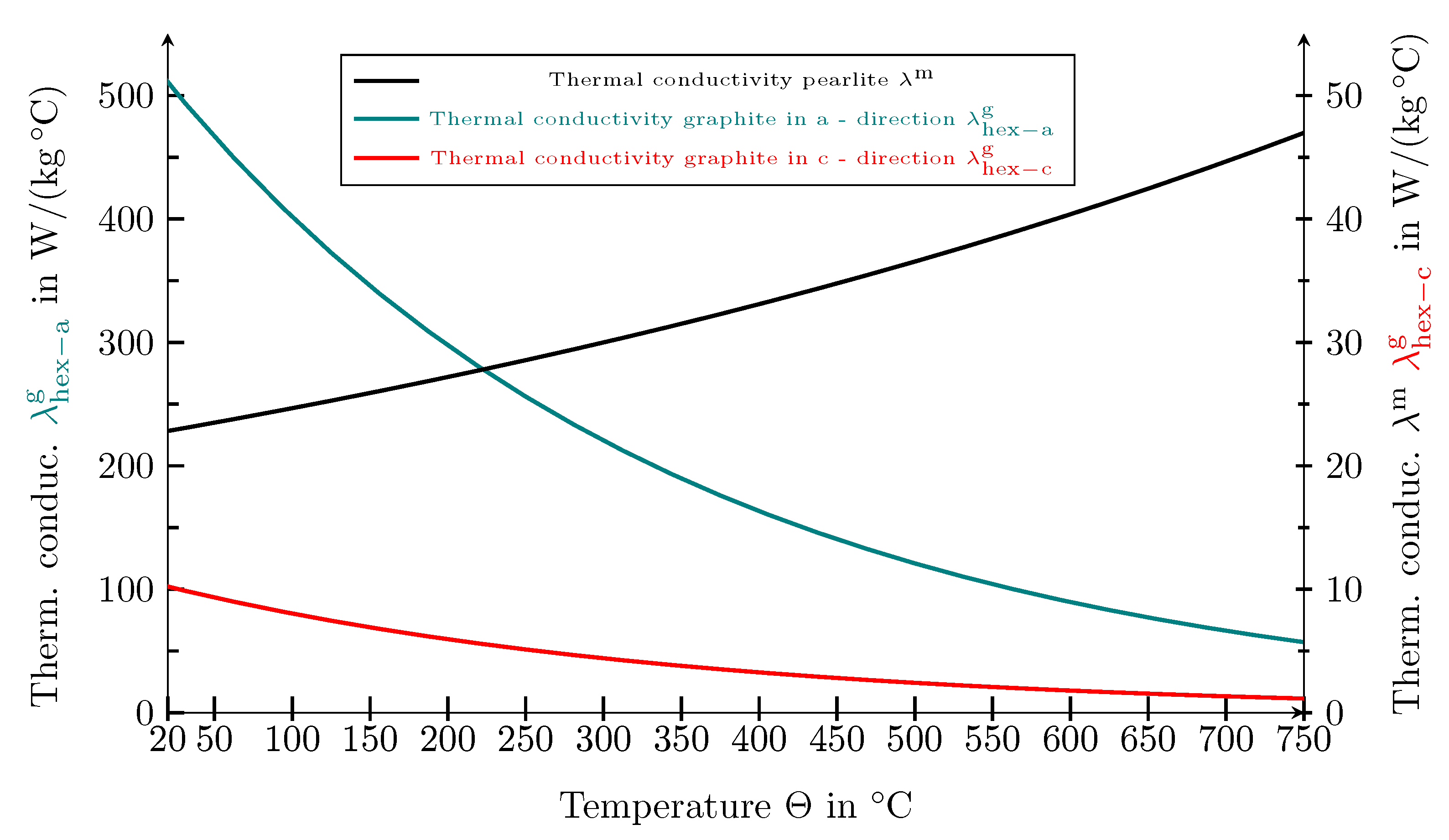
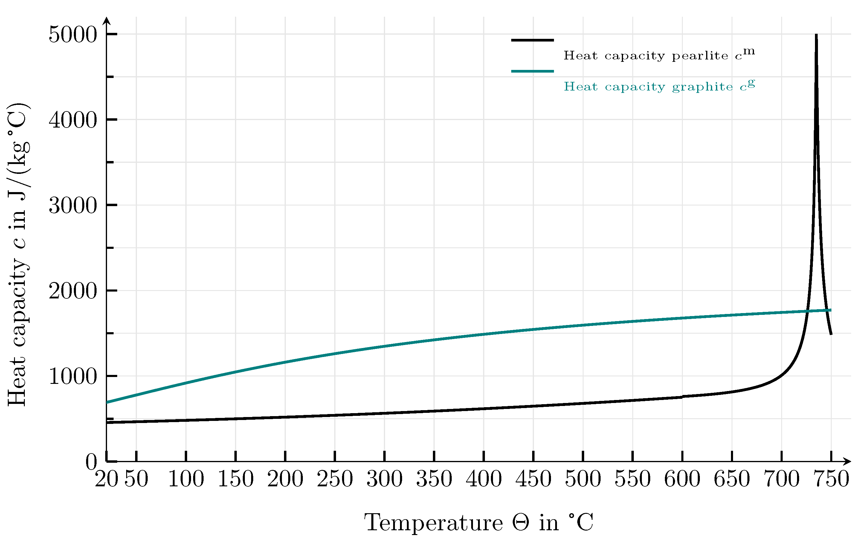
3.1. Mechanical and Thermal Model for Pearlite

The matrix of the cast iron is modelled as a homogeneous pearlitic material with isotropic properties. These simplifications are justified in Section 2. The mechanical behaviour of the pearlitic matrix is given by a rate-independent $J_2$ plasticity model with non-linear hardening, where the plastic hardening follows the so-called Voce law:

$$\begin{array}{c}\hfill {\sigma }_{\mathrm{y}}={\sigma }_{\mathrm{y},0}+({\sigma }_{\infty }-{\sigma }_{\mathrm{y},0})\left(1-exp(-\eta {\epsilon }_{\mathrm{akk}})\right).\end{array}$$

(4)

Kinematic hardening is not taken into account, which is due to the fact that the initial loading direction does not change during the numerical experiments. As small deformations are assumed, an additive decomposition of the strains is applied.

At room temperature, θ = 20 °C, a standard value for steels, $E^{\mathrm{m},\mathrm{RT}}=210\mathrm{GPa}$, is considered to be the Young’s modulus. The Poisson’s ratio of ${\nu }^{\mathrm{m}}=0.3$ is temperature-independent [29]. The yield strength of the pearlitic matrix is ${\sigma }_{\mathrm{y},0}^{\mathrm{m},\mathrm{RT}}=230\mathrm{MPa}$, which results from compression experiments. To define the model parameters for the saturating non-linear plastic hardening law, the publication of Allain and Bouaziz [30] is used. This work contains an empirical law for describing the plastic hardening of pure pearlite as a function of the interlamellar spacing between ferrite and cementite, which shows great agreement with experimental results. Allain and Bouaziz [30] found that interlamellar spacing has no influence on the saturation rate, but shifts the yield curves translationally with respect to the yield strength. The tensile strength and strain hardening parameters given by Allain and Bouaziz [30] serve at room temperature as saturation stress, ${\sigma }_{\infty }^{\mathrm{m},\mathrm{RT}}=772\mathrm{MPa}$, and saturation rate, ${\eta }^{\mathrm{m},\mathrm{RT}}=19\mathrm{GPa}$. As the strength and toughness of pearlitic steel is highly dependent on its morphology, it is important to emphasise that the choice of the matrix parameters is subject to uncertainty.

All mechanical material parameters of the pearlitic matrix introduced so far are valid at room temperature. The simulation study covers a temperature range from 20 to 750 °C. The determination of the material parameters at higher temperatures is described afterwards. Steel structures, with regard to their load-bearing capacity, have a high safety relevance in the construction industry. This applies especially to their design against failure at temperatures above room temperature, in order to prevent fatal incidents in the event of fires. For this reason, there are reliable standards and guidelines that describe the change of the mechanical parameters of structural steel as a function of temperature, relative to room temperature. A common standard in Europe is the Eurocode [31], while the USA uses structural fire protection [32]. Temperature-dependent changes of the different material parameters are herein given by reduction factors. The factors describe the ratio of a certain variable at elevated temperature in relation to its value at room temperature. There are large differences between the introduced references with regard to the reduction factors. Investigations by Kodur et al. [33] have shown that the reduction factors for the Young’s modulus and the yield strength of structural steel, mentioned in the Eurocode [31], are better than the equivalent factors in structural fire protection [32]. For the simulation study, the values contained in

Table 2. Temperature-dependent mechanical material parameters of the pearlitic matrix. Temperature $\theta$; reduction factor of the Young’s modulus, $k_{\mathrm{E}}$; Young’s modulus $E^{\mathrm{m}}$; reduction factor of the yield strength, $k_{\mathrm{y}}$; yield strength ${\sigma }_{\mathrm{y},0}^{\mathrm{m}}$; saturation stress ${\sigma }_{\infty }^{\mathrm{m}}$; saturation rate ${\eta }^{\mathrm{m}}$.

$\mathit{\theta }{[}^{\circ }\mathbf{C}]$	${\mathit{k}}_{\mathbf{E}}$	${\mathit{E}}^{\mathbf{m}}\left[\mathbf{GPa}\right]$	${\mathit{k}}_{\mathbf{y}}$	${\mathit{\sigma }}_{\mathbf{y},0}^{\mathbf{m}}\left[\mathbf{MPa}\right]$	${\mathit{\sigma }}_{\mathit{\infty }}^{\mathbf{m}}\left[\mathbf{MPa}\right]$	${\mathit{\eta }}^{\mathbf{m}}\left[\mathbf{GPa}\right]$
20	1.0	210.0	1.0	230.0	772.0	19.0
150	0.95	199.5	1.0	230.0	772.0	19.0
300	0.8	168.0	1.0	230.0	772.0	19.0
450	0.65	136.5	0.89	204.7	687.1	19.0
600	0.31	65.1	0.47	108.1	362.8	19.0
750	0.11	23.1	0.17	39.1	131.2	19.0

, corresponding to Eurocode [31], are used as reduction factors.

If no explicit reduction factor is given for a specific temperature at which simulations are carried out, linearly interpolated reduction factors with respect to temperature are used. The reduction factor of the Young’s modulus, $k_{\mathrm{E}}\left(\theta \right)$, is applied to the Young’s modulus of the pearlitic matrix at room temperature, $E^{\mathrm{m}}\left(\theta \right)=k_{\mathrm{E}}\left(\theta \right)E^{\mathrm{m},\mathrm{RT}}$, and the yield strength reduction factor, $k_{\mathrm{y}}\left(\theta \right)$, to the yield strength at room temperature, ${\sigma }_{\mathrm{y},0}^{\mathrm{m}}\left(\theta \right)=k_{\mathrm{y}}\left(\theta \right){\sigma }_{\mathrm{y},0}^{\mathrm{m},\mathrm{RT}}$. The temperature dependence of the saturation stress, ${\sigma }_{\infty }^{\mathrm{m}}\left(\theta \right)$, and the saturation rate, ${\eta }^{\mathrm{m}}\left(\theta \right)$, follow the procedure described in Bonora and Ruggiero [1]. Therein, each yield curve is assumed to be self-similar with respect to the material behaviour at room temperature, where the yield stress, ${\sigma }_{\mathrm{y}}^{\mathrm{m},\mathrm{RT}}$, is scaled with respect to the temperature-dependent yield strength. In Figure 5, the plastic flow curves are shown at different temperatures.

The thermal conductivity of pearlite has a weak transverse isotropy with regard to the orientation of the ferrite and cementite lamellae of a single pearlitic colony. Compared to the anisotropy of graphite, however, this anisotropy is negligible and is therefore not modelled. In Figure 6, the temperature-dependent isotropic thermal conductivity of the pearlitic matrix, ${\lambda }^{\mathrm{m}}$, is shown.

The parameters correspond to typical values of a eutectoid Fe-C system, with a carbon mass fraction of $0.8$ $\mathrm{m}.-\%$, taken from Helsing and Grimvall [34]. As the temperature-dependent specific heat capacity of the pearlitic matrix, values of steel given in Eurocode [31] are used, $c^{\mathrm{m}}$, as shown in Figure 7.

It should be noted that in the literature, the range of specific heat capacities for metallic materials is very wide. For an overview, for example, see Umino [35]. The mass density of the pearlitic matrix has the value ${\rho }^{\mathrm{m}}=7838\mathrm{kg}/{\mathrm{m}}^3$ [34], and is independent of temperature.

3.2. Mechanical and Thermal Model for the Graphite Lamellae

Graphite particles consist of many carbon layers, so-called basal planes or graphene layers, which are layered parallel on top of each other, in an AB sequence [36]. Individual basal planes consist of a large number of benzol rings, where carbon atoms are connected by strong covalent bonds in the a-direction of the hexagonal crystal system. There is significantly less molecular interaction between the different planes, which is caused by metallic bonding forces in the c-direction of the hexagonal crystal system [4,12,16,37]. The consequence of this crystal structure is a pronounced anisotropy of the mechanical properties and thermal conductivity [16,36,38]. If the covalent bonds within the basal planes are stressed, the lamellae exhibit much higher mechanical properties compared to stressing the weak metallic bonds between the planes [36]. Within the basal planes, thermal conductivity is also significantly greater than those orthogonal to them. In many models, lamellar graphite is assumed to be isotropic, which is the case in the work Metzger and Seifert [14], for example. In situ microtensile tests and numerical studies, Pina et al. [4], however, have shown that graphite isotropy has a major influence on the elastic–plastic behaviour of grey cast iron. It was also concluded that a numerical model with anisotropically modelled graphite reproduces the behaviour of cast iron quantitatively better than a model with isotropic graphite. Based on this information and considering its atomic structure, lamellar graphite is modelled as a transversely isotropic material that behaves linearly elastic, as also shown in the works [4,11,16,24]. The stresses are given by Hooke’s law, where the crystal orientations of the graphite lamellae are taken into account by transversal isotropic stiffness tensors, rotated in the $x,y,z$ reference coordinate system. During the algorithmic generation of the simulation domains, as shown in Section 2, the orientations of the graphite lamellae are stored and used to rotate the stiffness tensors of each graphite lamella.

In the literature, there is broad consensus that the tension–compression stress–strain asymmetry of grey cast iron is a consequence of graphite particles [11,12,13,14]. In Bonora and Ruggiero [1], however, it is pointed out that it is not enough to consider graphite as a permanent microcrack but it must be considered in a more complex way. The fact that the particles behave like cracks under tensile loading can be explained by two possible mesoscopic processes. On one hand, it can be explained as a result of microcrack formation within the graphite particles and/or as a result of the separation of the graphite–matrix transition region, on the other hand. For the two mesoscopic processes, different modelling approaches exist. In Norman and Calmunger [11], the tension–compression dependence is predominantly attributed to debonding processes, and a simple damage criterion, available in Abaqus, is used to describe the successive process. Microcracking, which essentially occurs within the graphite lamellae, explains the tension–compression dependence in the experimental work of Haenny and Zambelli [12]. To model the tension–compression dependence of graphite particles, a phenomenological approach is used in this work, where a domain, $\mathsf{\Omega }$, with $N\in \mathbb{N}$ graphite lamellae is considered. The approach is to degrade the transversely isotropic stiffness tensor of a graphite particle, ${\mathcal{C}}^{\alpha }$, with $\alpha \in \{1,\cdots ,N\}$, by scalar multiplication with a continuous function, $d^{\alpha }\left({\epsilon }_{\mathrm{vol}}^{\alpha }\right):\mathbb{R}\to (d_{\min },1)$, with $d_{\min }\in (0,1]$, of the form:

$$\begin{array}{c}\hfill d^{\alpha }\left({\epsilon }_{\mathrm{vol}}^{\alpha }\right)\left(t\right)=\frac{1-d_{\min }}{2}\left(1+tanh\left(\frac{-4{\epsilon }_{\mathrm{vol}}^{\alpha }\left(t\right)}{{\epsilon }_{\mathrm{vol}}^{\mathrm{crit}}}\right)\right)+d_{\min }.\end{array}$$

(5)

The upper index $\alpha$ is used to assign the degradation function to a particular graphite lamella, existing in the subset ${\mathfrak{B}}^{\alpha }\subset \mathsf{\Omega }$. Each degradation function has a continuous transition between the minimum degradation value $d_{\min }$ and one and depends on the effective volume change of a graphite particle:

$$\begin{array}{c}\hfill {\epsilon }_{\mathrm{vol}}^{\alpha }\left(t\right)=\frac{1}{V^{{\mathfrak{B}}^{\alpha }}}\underset{{\mathfrak{B}}^{\alpha }}{\int }\frac{\mathrm{tr}\left(\epsilon \left(\mathit{x}\right)\right)}{3}\mathrm{d}V.\end{array}$$

(6)

Using the first invariant of the strain tensor, $\epsilon$, the volume change of a material point is defined. The degradation function assumes its maximum value for ${\epsilon }_{\mathrm{vol}}^{\alpha }=-{\epsilon }_{\mathrm{vol}}^{\mathrm{crit}}\to d^{\alpha }(-{\epsilon }_{\mathrm{vol}}^{\mathrm{crit}})\approx 1$ and its minimum value, $d_{\min }$, for ${\epsilon }_{\mathrm{vol}}^{\alpha }={\epsilon }_{\mathrm{vol}}^{\mathrm{crit}}\to d^{\alpha }\left({\epsilon }_{\mathrm{vol}}^{\mathrm{crit}}\right)\approx d_{\min }$. The threshold value of the volume change, ${\epsilon }_{\mathrm{vol}}^{\mathrm{crit}}$, defines the transition width between the minimum and maximum value of the degradation function. Due to the fact that tensile stresses are characterised by positive volume changes, for the threshold value of the volume change, ${\epsilon }_{\mathrm{vol}}^{\mathrm{crit}}\in \mathbb{R}>0$ applies. An exemplary representation of the course of the degradation function is shown in Figure 8, where the meanings of the various function parameters are given.

Various influencing factors play an important role in the deformation of a graphite particle, such as the shape of the particle and its orientation with respect to the direction of loading, all of which are taken into account by means of the introduced model [4]. With this approach, it is not necessary to distinguish between the possible mesoscopic failure mechanisms of the graphite lamellae, namely debonding and microcrack formation. Furthermore, it is unnecessary to model crack closure processes, as these are intrinsically included in the presented procedure [14]. The degradation of the graphite stiffness, depending on the effective volume change of a graphite particle, is similar to the model described in Metzger and Seifert [14].

There are many publications that deal with the determination of the linear–elastic parameters of graphite. Although the material parameters differ, they are quite similar, which can be observed in [37,39,40,41], listed in

Table 3. Mechanical material parameters of the graphite lamellae.

	Pascal et al. [41]	Bosak et al. [40]	Blakslee et al. [39]
$C_{11}^{\mathrm{g}}$ in MPa	1126.0	1109.0	1060.0
$C_{12}^{\mathrm{g}}$ in MPa	200.0	139.0	180.0
$C_{13}^{\mathrm{g}}$ in MPa	39.5	0.0	15.0
$C_{33}^{\mathrm{g}}$ in MPa	40.7	38.7	36.5
$C_{44}^{\mathrm{g}}$ in MPa	4.51	5.0	0.18
$C_{66}^{\mathrm{g}}$ in MPa		485.0

. In this work, graphite lamellae possess the mechanical properties of monocrystalline graphite, as determined by Bosak et al. [40].

Investigations by Kelly [37] have shown that the temperature dependence of the component $C_{33}$, belonging to the transversely isotropic stiffness tensor of graphite, is negligible in the considered temperature range. Therefore, the elastic material parameters of graphite are assumed to be temperature-independent in the following, as was also the case the study of in Pina et al. [16]. In the particle-specific $\tilde{x},\tilde{y},\tilde{z}$ coordinate system, the transverse isotropic stiffness tensor of a specific graphite lamella is constructed in such a way that the third principal material direction is orthogonal to the longitudinal axes (c-direction of the hexagonal crystal lattice) of the graphite lamella.

From the wide range of published thermal conductivities for graphite (see Holmgren [38] for an overview) the temperature-dependent parameters given by Helsing and Grimvall [34] are used for the simulation study (Figure 6). Compared to the thermal conductivity, ${\lambda }_{\mathrm{hex}-\mathrm{c}}^{\mathrm{g}}$, running in the c-direction, the component of the transversely isotropic thermal conductivity of graphite, ${\lambda }_{\mathrm{hex}-\mathrm{a}}^{\mathrm{g}}$, running in the a-direction of the hexagonal crystal lattice, is up to an order of magnitude higher [38]. In order to take the crystal orientation of a graphite lamella into account, its transverse isotropic thermal conductivity is transformed into the $x,y,z$ reference coordinate system of the simulation domains. The mass density of the graphite particles is independent of temperature, ${\rho }_{}^{\mathrm{g}}=2200\mathrm{kg}/{\mathrm{m}}^3$ [34].

4. Mechanical Simulations

As simulation results, only macroscopic mechanical quantities of the SVEs, calculated according to Hill [42], are presented below. To calculate the effective thermal conductivity, the same procedure is used as that used by August et al. [43], but with a heterogeneous heat flow that takes into account the anisotropic thermal conductivity of the graphite particles.

4.1. Key Points of the Numerics and the Simulation Setup

An equidistant, orthogonal grid is used to spatially discretise the simulation domains.

All mechanical simulations are one-dimensional, moment-free tensile or compression tests on statistical volume elements (SVEs). In the loading direction, which is always parallel to an axis of the $x,y,z$ reference coordinate system, an orthogonal displacement is imposed as a mechanical boundary condition on both sides of the simulation domain, which freely allows tangential displacements. In the two other spatial directions, one side of the simulation domain is stress-free and the opposite side has an orthogonal displacement equal to zero, whereby tangential displacements are possible. Due to the described boundary condition, transverse contractions are possible without restrictions.

4.2. Analysis of the Mechanical Model

In Section 2, it is explained that cast iron with lamellar graphite behaves isotropically in macroscopic experimental tests. This is not the case for the SVEs used, as the simulation domains do not contain a sufficient number of transversely isotropic graphite particles for their anisotropy to be statistically eliminated. To investigate how strongly anisotropic the SVEs are, tensile tests are carried out on three different graphite morphologies of the SVEs IA2, IA3, IA4 and IA5, each with a graphite flake volume fraction of 10 $\mathrm{v}.-\%$ and at room temperature, θ = 20 °C. Figure 9 shows the resulting stress–strain diagrams under one-dimensional, moment-free tensile loading of each of the three variants of a graphite class. The corresponding standard deviations of the different graphite morphologies are given as a measure of anisotropy, in the form of error bars.

It can be seen that the average stress–strain curve of a certain graphite class has a smaller standard deviation as the average particle size decreases. This means that the anisotropy strength decreases for a constant domain size with a decreasing average particle size. This is due to the fact that the number of graphite particles in a SVE increases with smaller particles. For comparison, the statistical volume elements of the IA2 graphite class contain between 250 and 300 particles; in contrast, 5500 to 5800 particles are embedded in the IA5 simulation domains. To obtain the same number of particles within an SVE of the graphite class IA5 as in an SVE of the type IA2, the domain size of the IA2 SVE would have to be approximately 20 times larger than that of the IA5 SVE, which would increase the computational effort by the same factor.

In the following, the effect of the minimum value of the degradation function, $d_{\min }$, and the threshold value of the volume change, ${\epsilon }_{\mathrm{vol}}^{\mathrm{crit}}$, on the macroscopic stress–strain behaviour of one-dimensional tensile tests is investigated. The simulations are performed at room temperature, θ = 20 °C, on GJL-150 SVEs with a graphite flake volume fraction of 10 $\mathrm{v}.-\%$.

The minimum value of the degradation function is varied for the values $d_{\min }=\{0.05;0.06;0.07\}$, at a constant threshold of volume change of ${\epsilon }_{\mathrm{vol}}^{\mathrm{crit}}=0.001$. The resulting stress–strain plots for a one-dimensional, moment-free tensile load are shown in Figure 10.

The effective macroscopic stiffness of the SVE increases with increasing $d_{\min }$. The reason for this is that graphite particles have higher degraded stiffnesses as the minimum value of the degradation function increases, and thus the macroscopic stiffness of a volume element also increases.

For a constant minimum value of the degradation function of $d_{\min }=0.05$, the threshold of the volume change is varied for the values ${\epsilon }_{\mathrm{vol}}^{\mathrm{crit}}=\{0.00075,0.001,0.002\}$. The corresponding stress–strain curves for a one-dimensional, moment-free tensile load are shown in Figure 11.

It can be seen that the material behaviour does not change significantly in the investigated range of values.

For the simulation study, $d_{\min }=0.05$ is chosen as the minimum value of the degradation function and ${\epsilon }_{\mathrm{vol}}^{\mathrm{crit}}=0.1\%$ for the threshold value of the volume change. These values are equivalent to the parameters with the same meaning in Metzger and Seifert [14].

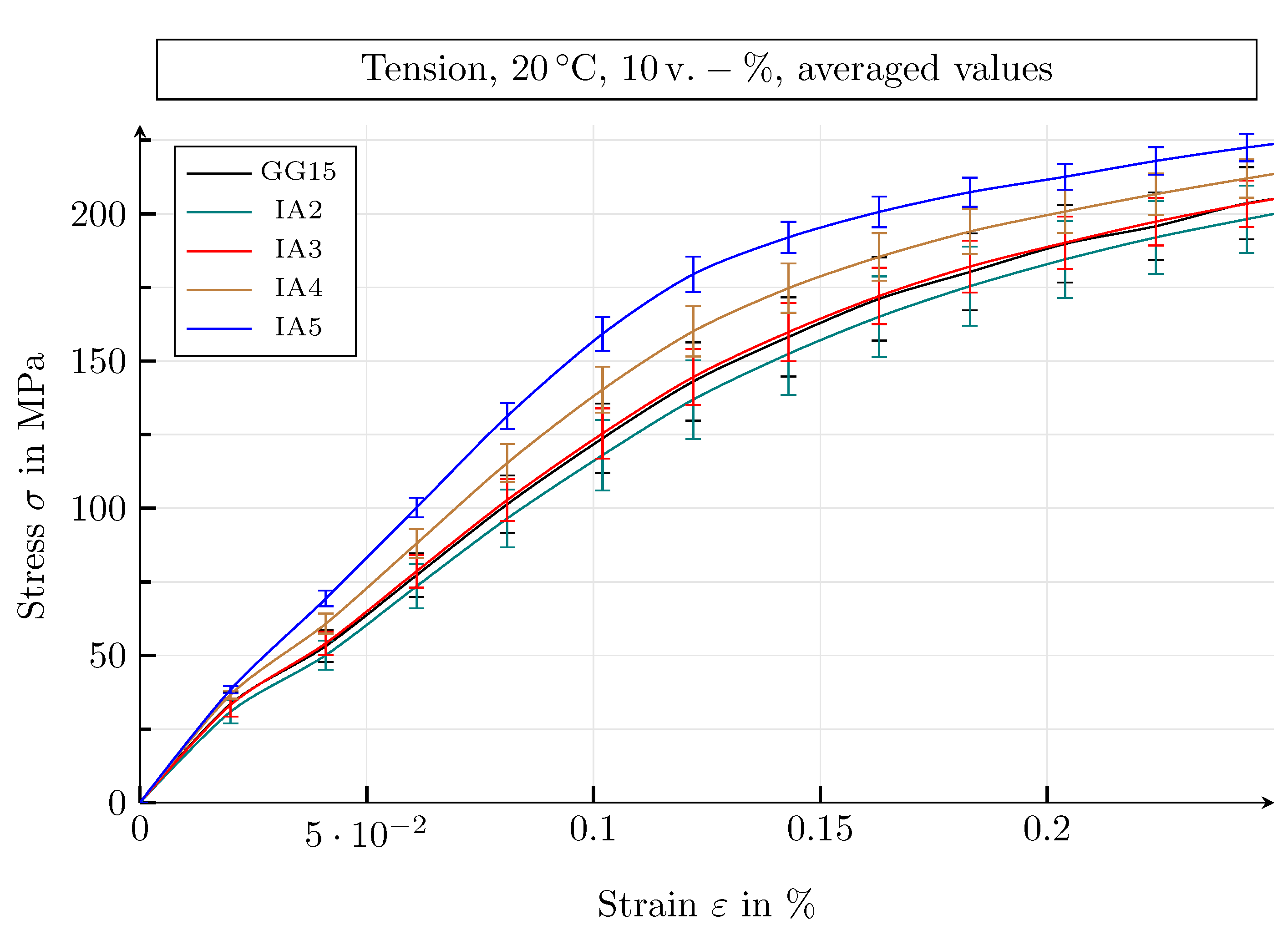
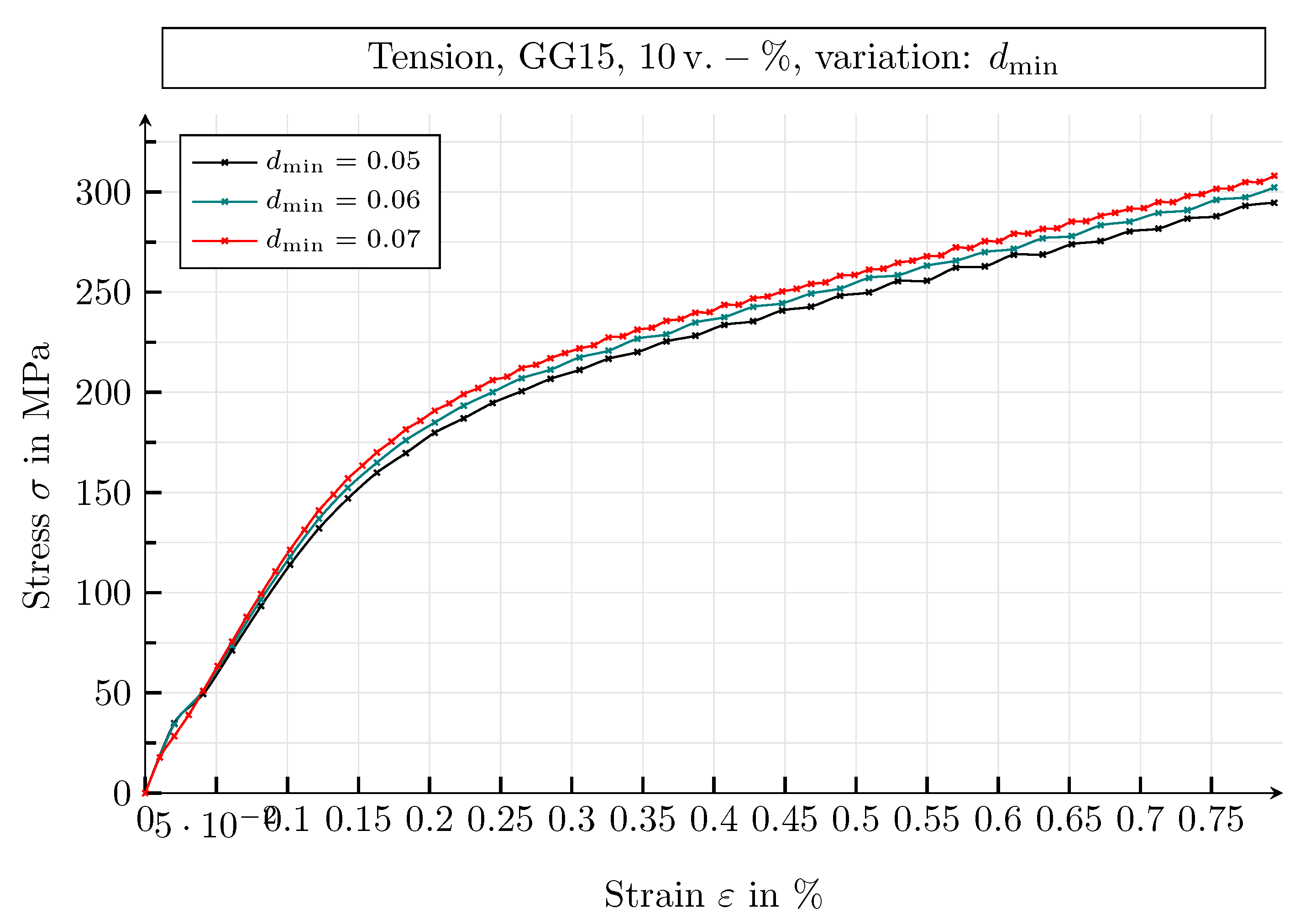
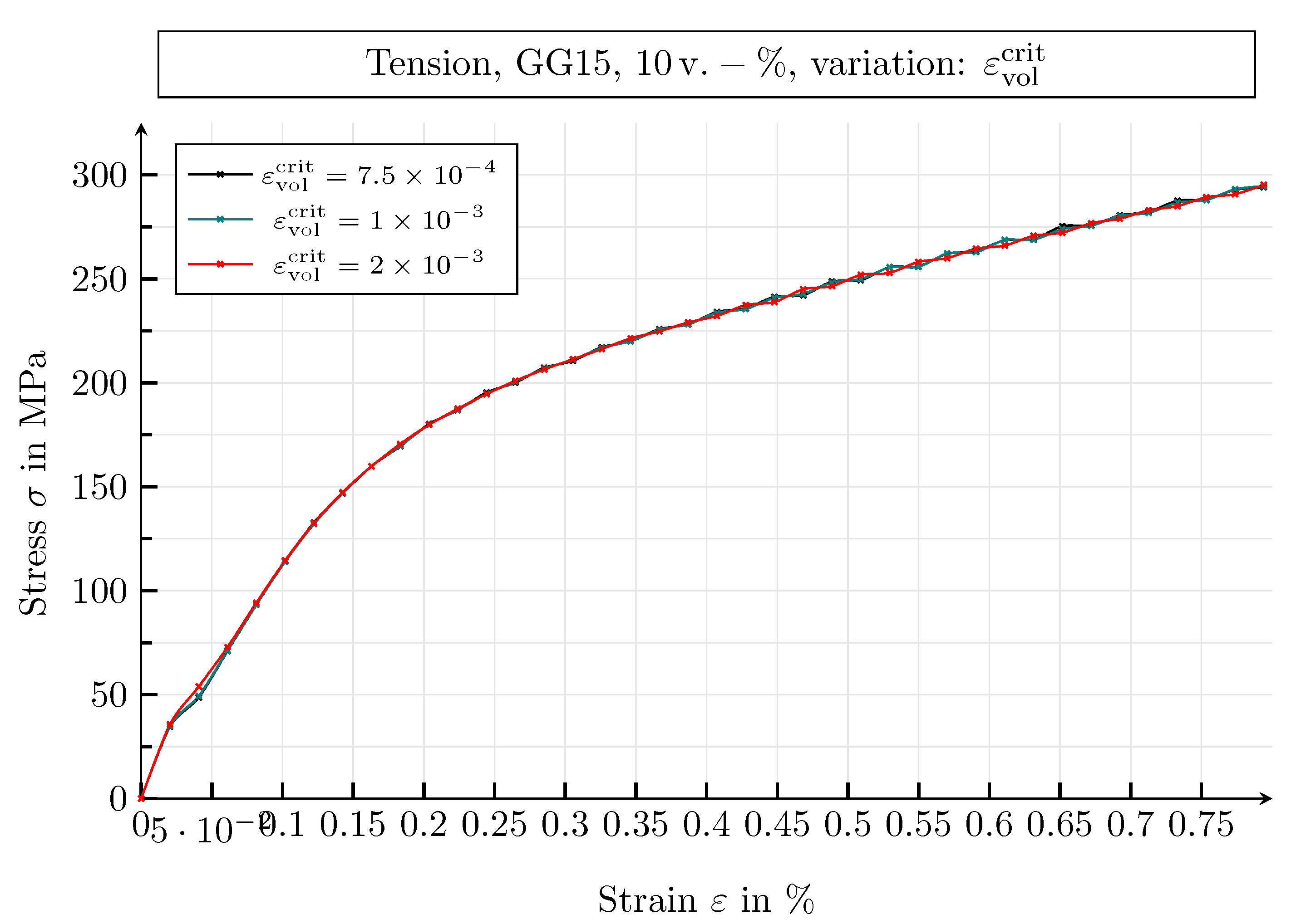
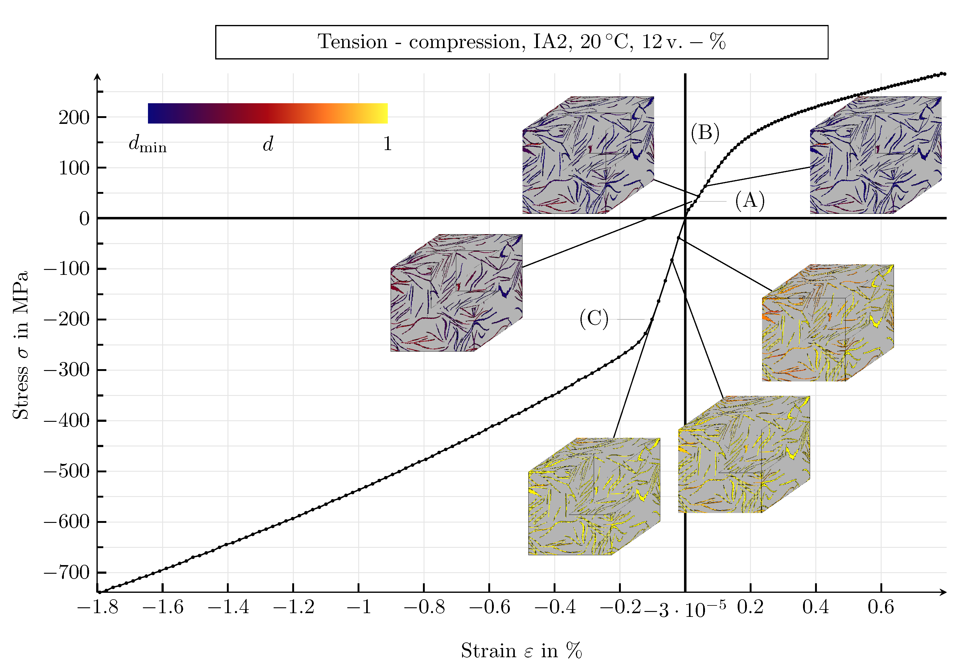
4.3. Mechanical Simulation Study

All material parameters of the following simulations are introduced in Section 3. The mechanical model parameters are identical to the parameters with the same meaning in Metzger and Seifert [14]: minimum value of the degradation function $d_{\min }=0.05$ and threshold value of the volume change ${\epsilon }_{\mathrm{vol}}^{\mathrm{crit}}=0.001$.

Figure 12 and Figure 13 show some typical characteristics of the tension–compression stress–strain asymmetric material behaviour of grey cast iron under tension and compression.

Figure 12 shows the stress–strain curves of a IA2 SVE with 12 $\mathrm{v}.-\%$ of graphite precipitations, at room temperature, for one-dimensional, moment-free tensile and compressive load. Contour plots of the degradation function, d, are given as an inlay. The pearlitic matrix occupies the grey areas within the contour plots.

In Figure 13, the material behaviour of grey cast iron, on the level of mechanical fields, is depicted. Shown are contour plots of the von Mises equivalent stress, ${\sigma }_{\mathrm{v}.\mathrm{M}.}$, and the accumulated plastic strain, ${\epsilon }_{\mathrm{akk}}$, at macroscopic tensile and compressive strains of equal magnitude, $\epsilon =0.0035$, running in the x direction.

Under tensile load, there is almost no linear range of the stress–strain curve in Figure 12. Starting at a strain of $\epsilon \sim 0.0002$, seen at point (A), the effective volume change of the graphite particles, ${\epsilon }_{\mathrm{vol}}^{\alpha }$, causes a significant degradation of the stiffnesses of the graphite particles. According to Equation (5), the region between point (A) and (B) is characterised by the continuous degradation of the graphite stiffnesses. As a result of mimicking microcrack formation and/or interface debonding, a disturbance of the force flow occurs. The stress concentrations occurring on the edges of the graphite lamellae cause local plastic deformations, as shown in Figure 13 (figures of tensile stresses), which leads to a further non-linear course of the stress–strain curve at macroscopically small strains. The observations described are typical characteristic of cast iron with lamellar graphite under tensile loading [12]. According to Noguchi and Shimizu [23], grey cast iron does not show a pronounced yield strength under tensile loading and breaks at a strain between $\epsilon =0.005$ and $0.01$, without visible necking at maximum stress.

The material behaviour under compressive load is completely different from that under tensile load. Up to a strain of $\epsilon \sim 0.001$, point (C) in Figure 12, there is a clearly identifiable linear section of the stress–strain curve. From the inserted contour plots of the graphite degradation, it can be seen that degradation only occurs in a few particles under compressive loading, since predominantly negative values of the effective volume changes, ${\epsilon }_{\mathrm{vol}}^{\alpha }$, are present. As a result, the force flow through the graphite particles is only slightly disturbed and hardly any stress concentrations occur on their edges, as shown in Figure 13 (figures of compressive loading). For macroscopic strains of equal magnitude, a more homogeneous stress field is present under compressive loading and plastic strains occur in larger areas of the matrix, cf. Figure 13. It can be seen that the tension–compression stress–strain asymmetry leads to a higher Young’s modulus and a higher yield strength under compressive load.

The characteristics described occur in all graphite morphologies and for all temperatures, but are more or less pronounced.

Figure 14 shows contour plots of the von Mises equivalent stress, ${\sigma }_{\mathrm{v}.\mathrm{M}.}$, and the accumulated plastic strain, ${\epsilon }_{\mathrm{akk}}$, of SVEs of the graphite classes GJL-150, IA2, IA3, IA4 and IA5, for a graphite flake volume fraction of 10 $\mathrm{v}.-\%$ and a temperature of $\theta =20{}^{\circ }\mathrm{C}$. The contour plots show the results of a macroscopic tensile strain of $\epsilon =0.0035$, in the x direction.

In all graphite morphologies, the graphite lamellae already lose their ability to transmit forces at a small macroscopic strain. It can be observed that with smaller graphite particles on average, both the contour plots of the von Mises equivalent stress and those of the accumulated plastic strain are more homogeneous. Finer graphite structures lead to more homogeneous mechanical fields [12].

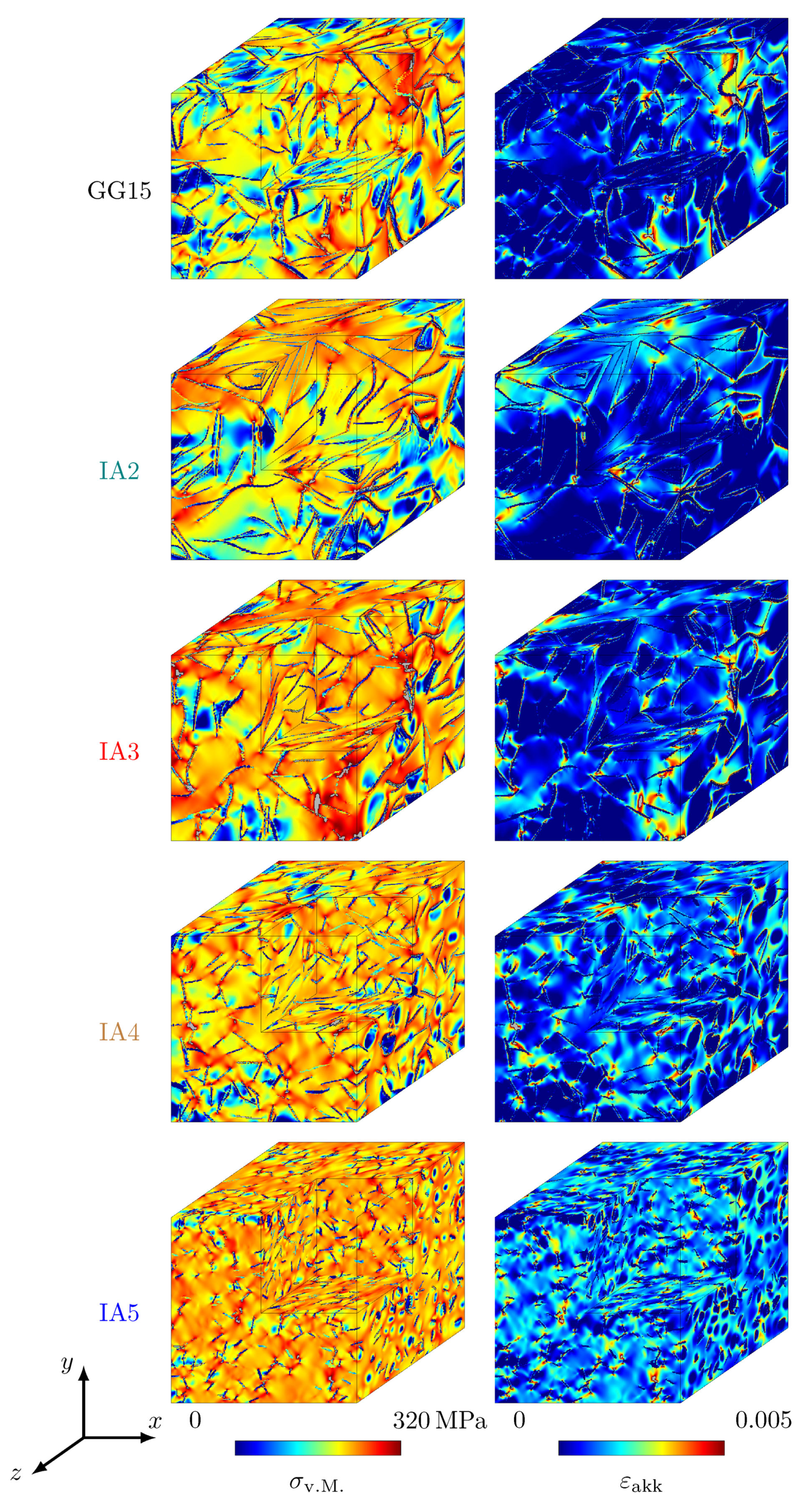
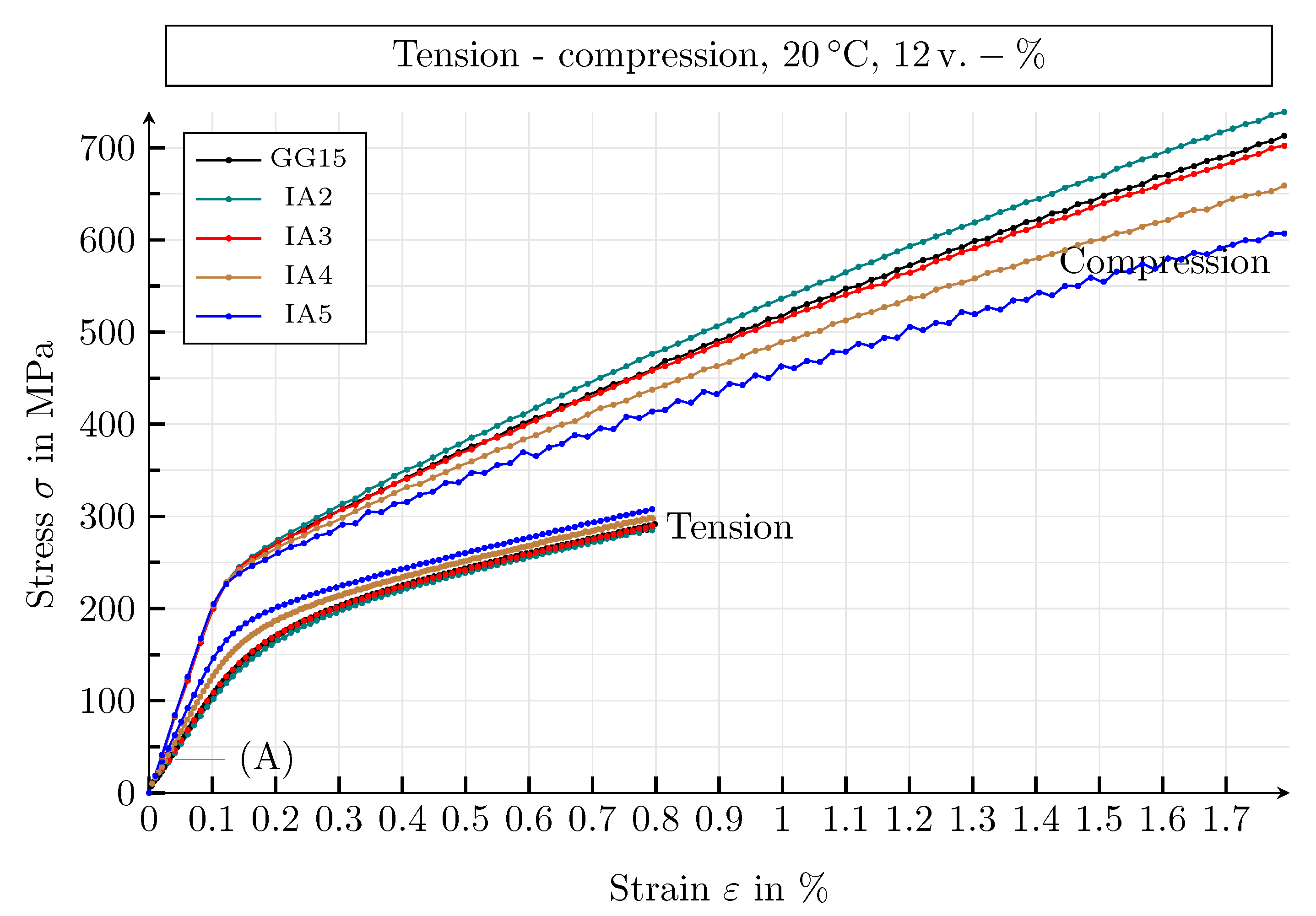
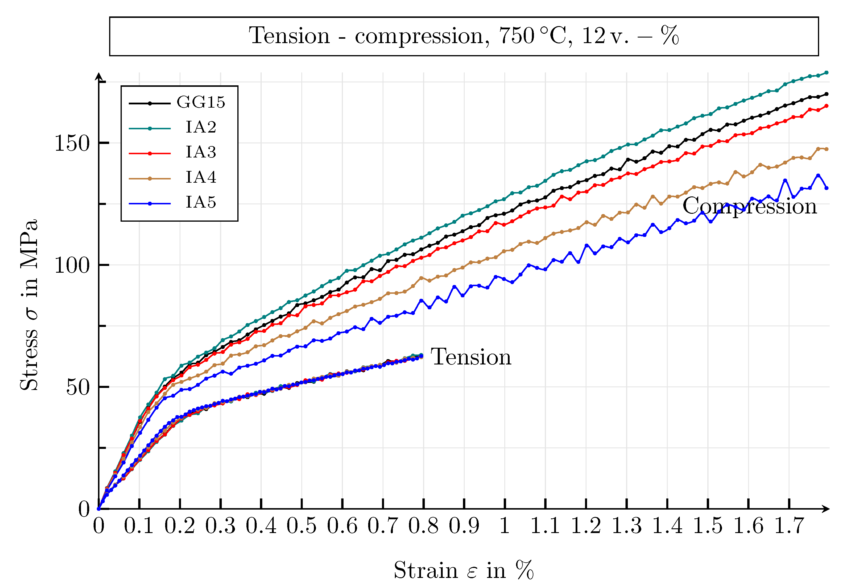
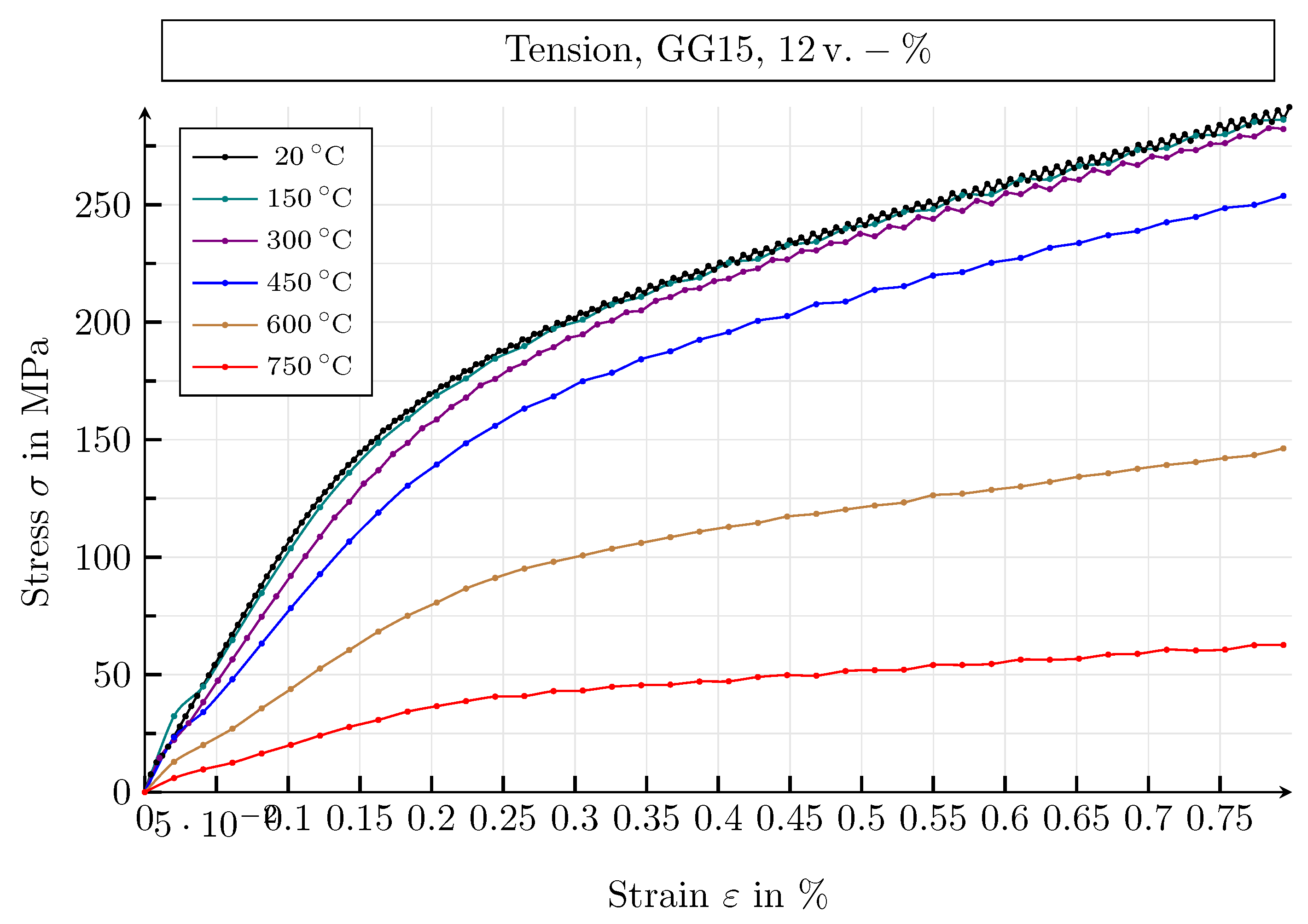
4.3.1. Results of the Mechanical Simulation Study

A detailed simulation study was carried out to investigate the influence of the graphite class and the graphite volume fraction on the macroscopic mechanical properties of cast iron with lamellar graphite. The study includes simulations of SVEs of every possible permutation of the graphite morphologies GJL-150, IA2, IA3, IA4 and IA5 [17], with graphite flake volume fractions of 10, 11 and 12 $\mathrm{v}.-\%$. The carbon mass fraction of GJL-150 is assumed to be in the range of $3.7$ to $3.9$ $\mathrm{m}.-\%$. With a mass density of ${\rho }^{\mathrm{m}}=7838\mathrm{kg}/{\mathrm{m}}^3$ [34] for the pearlitic matrix and ${\rho }_{}^{\mathrm{g}}=2200\mathrm{kg}/{\mathrm{m}}^3$ [34] for graphite, respectively, this leads to volume fractions of the graphite lamellae from 10 to 12 $\mathrm{v}.-\%$, as in Pina et al. [16]. For each possible variant of the SVEs, one-dimensional, moment-free tensile tests were carried out for the temperatures $\theta =\{20{}^{\circ }\mathrm{C},150{}^{\circ }\mathrm{C},300{}^{\circ }\mathrm{C},450{}^{\circ }\mathrm{C},600{}^{\circ }\mathrm{C},750{}^{\circ }\mathrm{C}\}$.

At the same temperatures, compression tests were simulated for all SVEs with a graphite flake volume fraction of 12 $\mathrm{v}.-\%$.

The most significant findings of the simulation study are explained below. If similar trends occur for different graphite classes, volume fractions or temperatures, this is pointed out; otherwise, the trend is only analysed using one simulation example. For a clearer representation, the stress–strain curves of the simulations under compressive load are given by positive values.

The simulation study was executed using combined methods of the morphology simulation framework Pace3D [44] (https://www.iam.kit.edu/cms/5317.php accessed 26 September 2021) and the data science compendium provided within the research data infrastructure Kadi4Mat [45] (https://www.kadi.iam-cms.kit.edu/ accessed 26 September 2021). In addition to the components required for performing the simulation study, such as a workflow manager and the repository, the research data infrastructure also includes methods from the data science area. The use of Kadi4Mat allows all simulations to be carried out in an automated and reproducible way, enabling to apply the FAIR principles [46]. The workflow includes for-each-loops that process any graphite class, any graphite volume fraction and any temperature. Using the loops, any component of the simulation study can be run on a remote high-performance computer. Utilising the API developed specifically for Kadi4Mat, the large data volumes of the simulations can then be stored as morphology look-up tables on the repository in a reusable way and shared with collaborators through the creation of records. With the introduced numerical methods and the use of Kadi4Mat, the already conducted simulation study can be very easily extended in further work, or other materials can be investigated without great effort. An exemplary diagram of such a Kadi4Mat-workflow is shown in Figure 15.

A comparison of the material behaviour of all graphite classes with 12 $\mathrm{v}.-\%$ of graphite precipitations, at tensile as well as compressive load and room temperature, is given in Figure 16. The stress–strain curves of the different SVEs differ only slightly when subjected to a tensile load up to a strain of $\epsilon \sim 0.0002$, which can be seen at point (A) in Figure 16. This effect occurs because the effective volume change of the graphite particles, ${\epsilon }_{\mathrm{vol}}^{\alpha }$, does not cause a significant degradation of the stiffnesses of the lamellar graphite at strains smaller than the threshold value of the volume change, ${\epsilon }_{\mathrm{vol}}^{\mathrm{crit}}$, and therefore the graphite morphology has no huge influence. It can be observed that the difference between the stress–strain curves increases after point (A). Under tensile load, the macroscopic mechanical properties increase with decreasing average particle size. The graphite class IA5 has the highest Young’s modulus and the highest yield strength, while the class IA2 has the lowest Young’s modulus and the lowest yield strength. Quantitative values of these parameters are shown later. Thus, the average particle size of an SVE clearly influences the stress–strain curves. The non-idealised GJL-150 SVE results in a stress–strain curve that lies between those of IA2 and IA3. It can be observed that the difference between the characteristics IA2 and IA3 is significantly smaller than that between IA4 and IA5. This is due to the fact that the changes between the average length of particles from IA2 to IA5, as shown in Table 1, influence the mean volume of the graphite particles cubically and accordingly, the number of particles in the simulation domain does not change linearly.

The stress–strain curves for compressive load have a clear, pronounced linear section. In the linear segment, the curves of all SVEs are very similar, and the yield strengths are also almost identical. Thus, the graphite class only has a noticeable influence on the macroscopic material behaviour of the cast iron material for stresses above the yield strength. This can be explained by the fact that under compressive load, there are hardly any positive effective volume changes of the graphite particles, ${\epsilon }_{\mathrm{vol}}^{\alpha }$, and thus there is only very little degradation of the graphite particles. The macroscopic material behaviour is therefore predominantly dominated by the matrix material. This phenomenon can also be observed in the experimental results. A clear influence of the graphite class can only be seen in the case of macroscopic plastic deformation. As soon as a non-linear material behaviour occurs, the stress–strain curves of the different SVEs differ significantly. In contrast to the tensile load, the graphite class IA2 has the highest stress–strain curve, while the graphite class IA5 has the lowest. Under compressive load, the characteristic curve of the GJL-150 SVE also runs between those of the graphite class IA2 and IA3.

Figure 17 shows the simulation results for the tensile and compressive load of the same SVEs as before, but at the temperature of $\theta =750{}^{\circ }\mathrm{C}$.

Compared to room temperature, the course of the individual stress–strain curves does not change qualitatively at elevated temperatures. In general, under tensile load, the differences between the stress–strain behaviour in the graphite classes become smaller with increasing temperature. If the temperature is 750 ${}^{\circ }\mathrm{C}$, there is hardly any difference between the curves anymore. The reason for this is that the stiffness of the pearlitic matrix decreases with increasing temperature and thus becomes similar to that of the degraded graphite, resulting in the fact that the influence of graphite on the macroscopic material behaviour disappears, since the mechanical fields are more homogeneous at higher temperatures.

Such a phenomenon is not present under compressive load. In contrast to the tensile simulations, the curves of the different volume elements do not adapt to one another with increasing temperature, since only a few graphite particles are degraded under compressive load.

Figure 18 shows the stress–strain curves of a GJL-150 SVE with 12 $\mathrm{v}.-\%$ of graphite precipitations, under tensile load, for the temperatures $\theta =\{20{}^{\circ }\mathrm{C},150{}^{\circ }\mathrm{C},300{}^{\circ }\mathrm{C},450{}^{\circ }\mathrm{C},600{}^{\circ }\mathrm{C},750{}^{\circ }\mathrm{C}\}$.

The quantitative progression of the curves is the same for all temperatures, but is developed to different degrees. As already described above, a very small linear section is followed by a region with a not strictly monotonic slope, which subsequently results in a pronounced non-linear material behaviour. The stress–strain curves decrease with increasing temperature, which is caused by the temperature-dependent material parameters of the pearlitic matrix, as shown in Table 2. However, up to a temperature of $\theta =450{}^{\circ }\mathrm{C}$, the drop in the characteristic curves is not significant, since for the temperatures $\theta =\{20{}^{\circ }\mathrm{C},150{}^{\circ }\mathrm{C},300{}^{\circ }\mathrm{C}\}$ only the Young’s modulus changes and not the yield strength and the strain hardening parameters of the matrix, as shown in Table 2.

As before for tensile load, the influence of temperature on the macroscopic behaviour of the same SVE is similar for compressive load, as shown in Figure 19.

With increasing temperature, the absolute stress values of the curves become smaller, whereby the difference between $\theta =20{}^{\circ }\mathrm{C}$, 150 and 300 ${}^{\circ }\mathrm{C}$ is low. In general, the course of the curve under compressive load is similar to that of a typical ductile steel, as there is a clearly identifiable linear region, which is followed by a non-linear plastic section.

Finally, the influence of the graphite volume fraction on the mechanical material properties is considered. Figure 20 shows the stress–strain curves for tensile and compressive load of a graphite morphology of type GJL-150, for the graphite flake volume fractions of $10 \mathrm{v}.-\%,11 \mathrm{v}.-\%$ and $12 \mathrm{v}.-\%$.

It can be observed that the curves have lower stress values under tensile load, with an increasing graphite volume fraction. Both the Young’s modulus and the yield strength decrease as the volume fraction of graphite increases. This fact is consistent with results and data from publications by Collini et al. [6], Haenny and Zambelli [12] and Noguchi and Shimizu [23], for example. This phenomenon can be explained by the increase in graphite, which weakens the matrix within an SVE.

Under compressive load, the behaviour is just the opposite, as a higher graphite volume fraction leads to higher mechanical properties. In this loading case, only a few graphite stiffnesses are degraded and have a positive effect on the macroscopic material behaviour of the SVEs, as graphite has a higher stiffness than the pearlitic matrix in the non-degraded state.

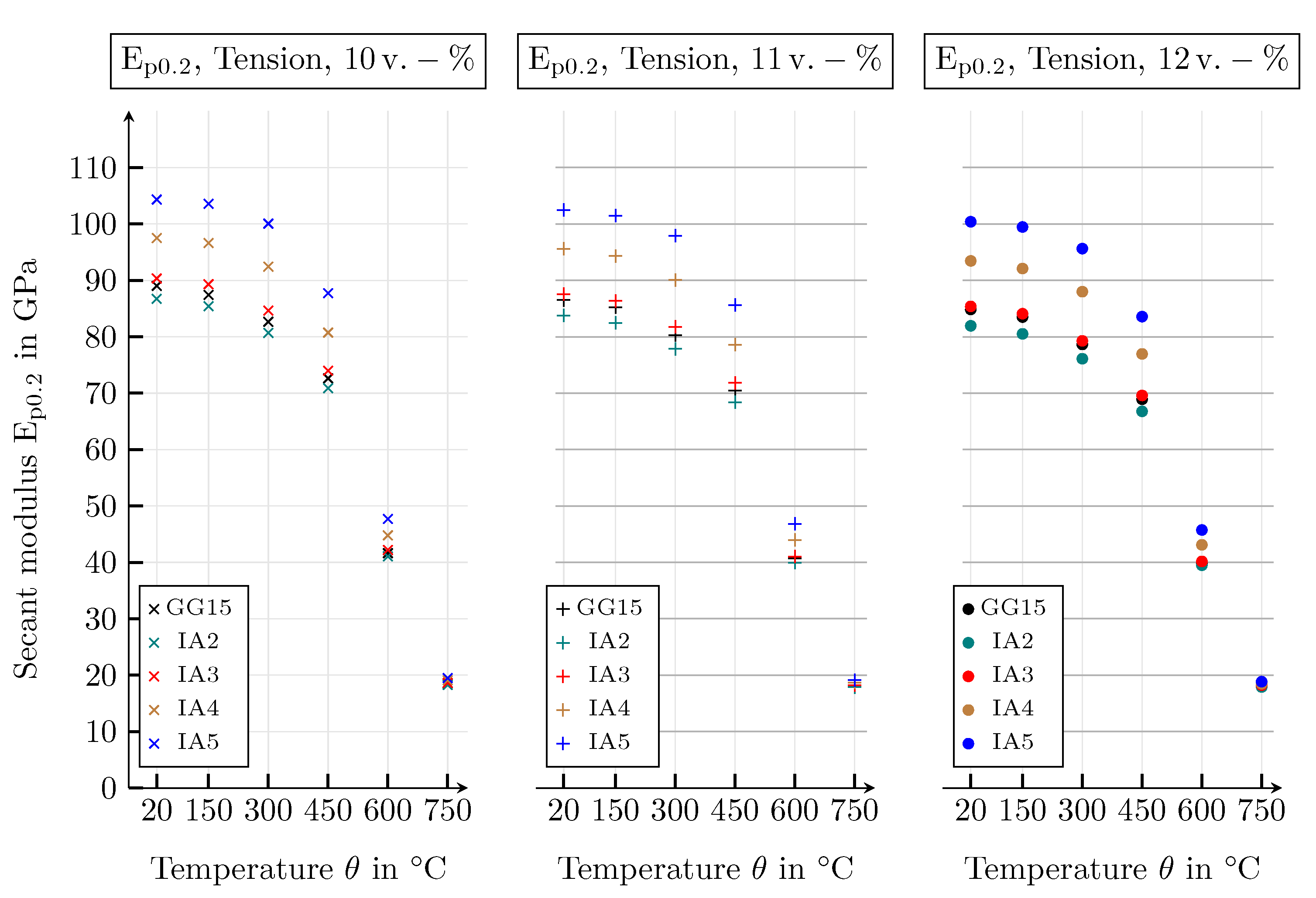
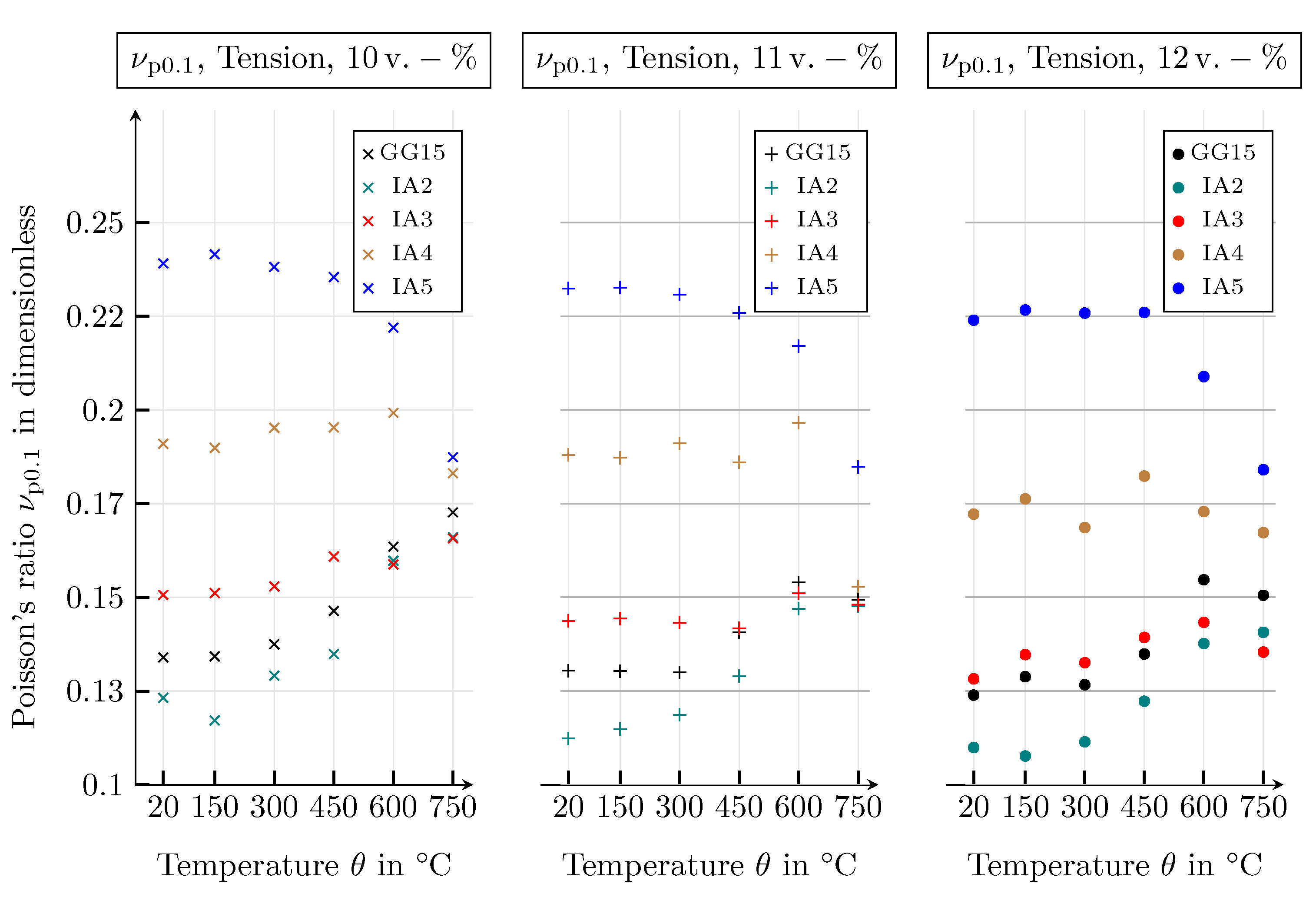
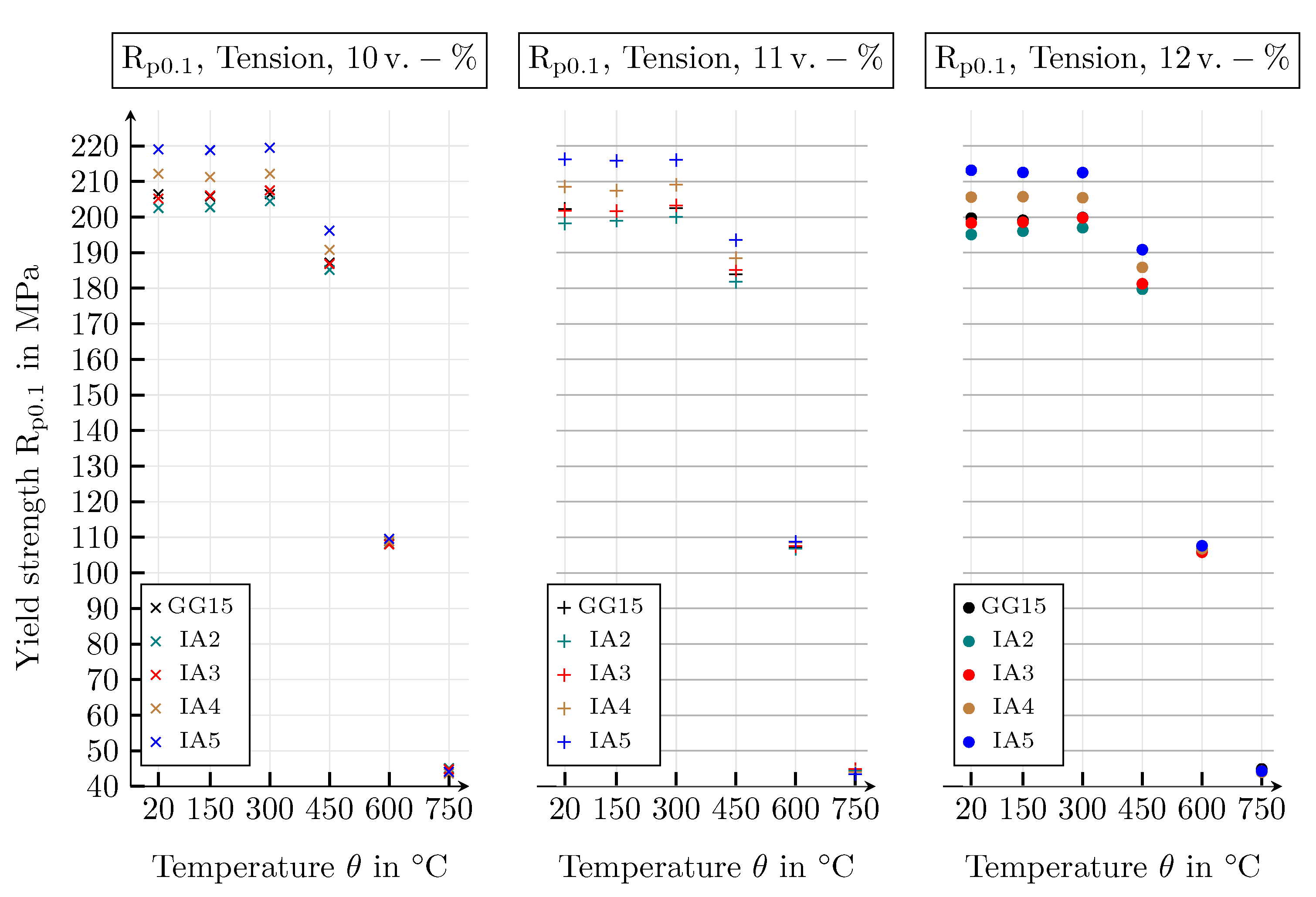
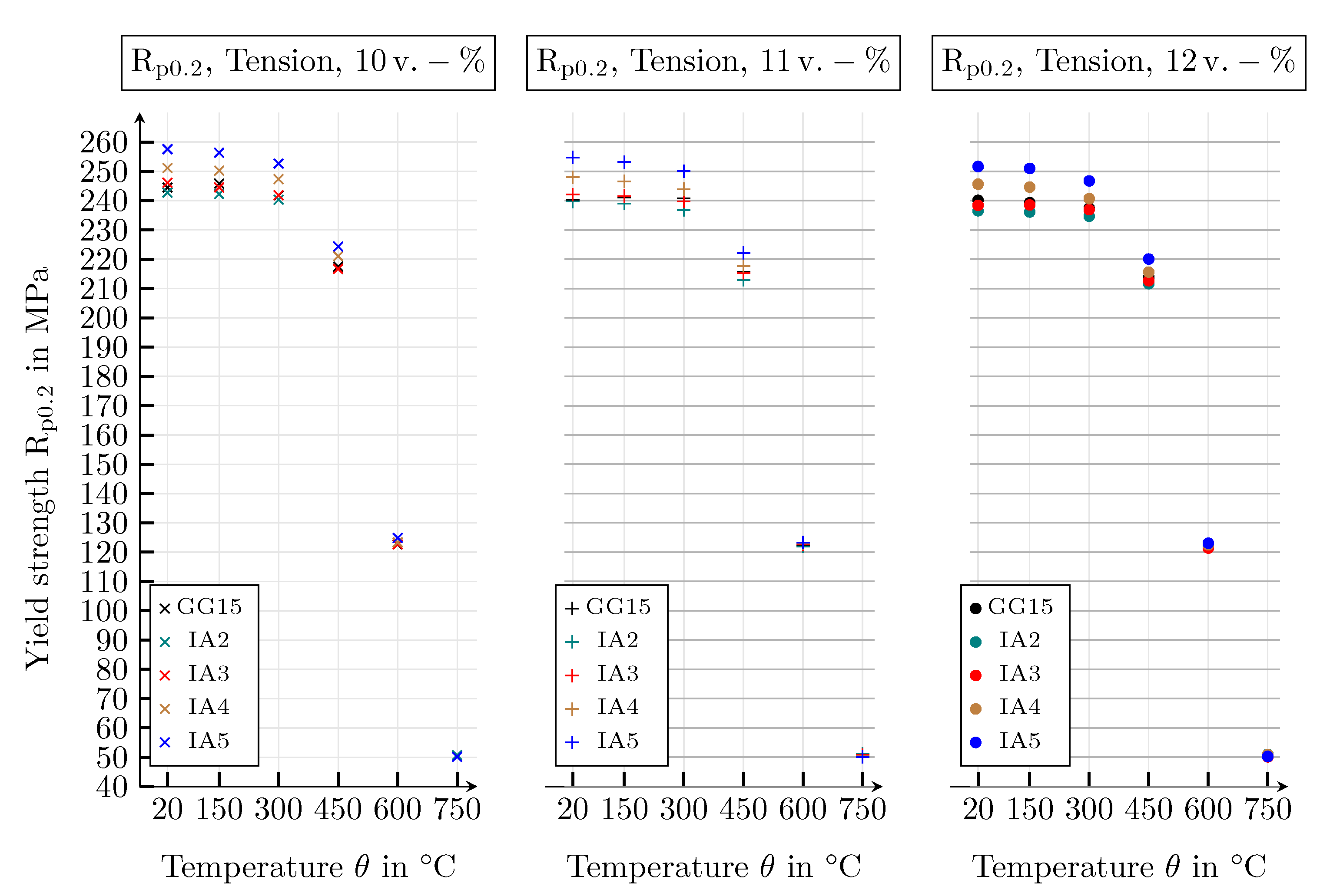
4.3.2. Mechanical Parameters

The simulation results are used to determine Young’s moduli, Poisson’s ratios and yield strengths, whereby it is assumed that the SVEs behave isotropically, which means that Hooke’s law applies, and that a one-dimensional stress state always exists.

In principle, the Young’s modulus of a material is given by the slope of the linear section of a stress–strain curve, at the onset of uniaxial, moment-free tensile loading. The yield strength marks the end of the linear section, and thus the transition of a material from elastic to plastic behaviour. In cast iron materials, however, such a linear section is not clearly pronounced, which makes it difficult to determine Young’s moduli and the yield strengths [47]. According to ASTME111 [48], the calculation of Young’s moduli, in terms of the tangent or secant modulus, is permissible for materials with non-linear elastic stress–strain characteristics. Depending on the strain at which the Young’s moduli are evaluated, these procedures for identifying these moduli lead to different results. In this work, the evaluation of Young’s moduli, at strains of $\epsilon =0.1\%$, ${\mathrm{E}}_{\mathrm{p}0,1}$, and $\epsilon =0.2\%$, ${\mathrm{E}}_{\mathrm{p}0,2}$, is performed in terms of the secant modulus. Poisson’s ratios are also determined at the same strain values, ${\nu }_{\mathrm{p}0,1}$ and ${\nu }_{\mathrm{p}0,2}$. To avoid difficulties in the determination of yield strengths, technical yield strengths, ${\mathrm{R}}_{\mathrm{p}0,1}$ and ${\mathrm{R}}_{\mathrm{p}0,2}$, are defined at the same strains [49]. In addition, due to the tension–compression stress–strain asymmetry, a distinction is made between Young’s moduli, Poisson’s ratios and yield strengths under tensile and compressive load. Figure 21 shows the procedure for determining the secant moduli and technical yield strengths.

Figure 22, Figure 23, Figure 24, Figure 25, Figure 26 and Figure 27 list the resulting Young’s modulus, Poisson’s ratios and yield strengths under tensile load. All corresponding parameters under compressive load are given in Figure 28 and Figure 29. It can be observed that under tensile load, all parameters decrease with an increasing graphite volume fraction. The same applies to an increasing average graphite particle size for the Young’s modulus and the yield strengths, whereas the opposite is valid for the Poisson’s ratios. With increasing temperature, the difference between the parameters in the different graphite morphologies becomes smaller under tensile load. The reason for this is, as already mentioned, that the stiffness of the pearlitic matrix is reduced with increasing temperature, and thus becomes similar to that of the degraded graphite. For compressive loading, this phenomenon does not significantly occur, as fewer graphite particles are degraded, making their influence on the macroscopic material behaviour much smaller. In addition, an increasing volume fraction of the graphite particles has a positive effect on the Young’s modulus and the yield strengths under compressive load, since the predominantly non-degraded graphite lamellae have a higher stiffness than the pearlitic matrix. The different parameters for tensile and compressive load are characteristic of tension–compression stress–strain asymmetrical materials. The parameters of the idealised IA3 SVE are most similar to the GJL-150 morphology.

At room temperature, under tensile load, the following values result in the secant moduli of the GJL-150 SVEs: ${\mathrm{E}}_{\mathrm{p}0,1}^{10\mathrm{v}.-\%}=112\mathrm{GPa}$, ${\mathrm{E}}_{\mathrm{p}0,2}^{11\mathrm{v}.-\%}=108\mathrm{GPa}$, ${\mathrm{E}}_{\mathrm{p}0,2}^{12\mathrm{v}.-\%}=106\mathrm{GPa}$. This is in good agreement with the literature, where values of $E=78$ to $103\mathrm{GPa}$, for example, are given for a GJL-150 material [50]. There is also good agreement between the Poisson’s ratio of the simulation results of the GJL-150 material under compressive loading, ${\nu }_{\mathrm{p}0,1}^{12\mathrm{v}.-\%}=0.246$, and the literature, $\nu =0.26$ [50]. The yield strengths result in the values ${\mathrm{R}}_{\mathrm{p}0,1}^{10\mathrm{v}.-\%}=206\mathrm{MPa}$, ${\mathrm{R}}_{\mathrm{p}0,1}^{11\mathrm{v}.-\%}=202\mathrm{MPa}$ and ${\mathrm{R}}_{\mathrm{p}0,1}^{12\mathrm{v}.-\%}=199\mathrm{MPa}$, which are comparable with values found in the literature of ${\mathrm{R}}_{\mathrm{p}0,1}=98$ to $165\mathrm{MPa}$ [50].

5. Thermal Simulations

A simulation study was performed to investigate the influence of the graphite class and the graphite volume fraction on the thermal properties of cast iron with lamellar graphite. The study includes simulations of SVEs of each possible permutation of the graphite classes GJL-150, IA2, IA3, IA4 and IA5 [17], with graphite flake volume fractions of 10, 11 and 12 $\mathrm{v}.-\%$, for the temperatures $\theta =\{20{}^{\circ }\mathrm{C},150{}^{\circ }\mathrm{C},300{}^{\circ }\mathrm{C},450{}^{\circ }\mathrm{C},600{}^{\circ }\mathrm{C},750{}^{\circ }\mathrm{C}\}$.

The simulation study includes the calculation of thermal equilibrium states, under the influence of heat conduction, as the only type of heat transfer. In the performed simulations, only a slight local change in the temperature of a material point can be observed, which is why the local thermal conductivity and the heat capacity are considered to be constant during one simulation. The thermal conductivity model is not verified, as it is a well-established and often used “standard model”.

The temperatures on two opposite boundaries of an SVE are set as constant but different, whereas the boundary conditions of the remaining boundaries are set as adiabatic. For example, if the top of an SVE has the constant temperature ${\theta }_{\mathrm{T}}$ and the bottom ${\theta }_{\mathrm{B}}$, when ${\theta }_{\mathrm{T}}\ne {\theta }_{\mathrm{B}}$ does apply, a constant heat flux is established between the top and bottom surfaces, at equilibrium. Based on this, the effective thermal conductivity of a heterogeneous material can be calculated using the method presented by August et al. [43], whereby the calculation of the heat flux is carried out by including the tensorial thermal conductivity of the graphite. The calculated thermal conductivities are shown in Figure 30.

According to Hecht et al. [51], a higher thermal conductivity in structures with longer graphite lamellae is the result of a larger proportion of basal planes, available for thermal conduction. The same argumentation results in an increasing effective thermal conductivity in SVEs with an increasing quotient between the height of the lamellae and the longitudinal axes of the lamellae [3,38]. These statements are also reflected by the simulation results. In Figure 30, it can be observed that the thermal conductivity of the SVEs increases when the average size of the graphite particles increases from IA5 to IA2. As already observed in Holmgren [38], it can be seen that the thermal conductivity of grey cast iron decreases with increasing temperature.

The thermal conductivity of the GJL-150 SVEs results in the following values for $\theta =150{}^{\circ }\mathrm{C}$: ${\lambda }^{10\mathrm{v}.-\%}=41.53\mathrm{W}/\left(\mathrm{m}\mathrm{K}\right)$, ${\lambda }^{11\mathrm{v}.-\%}=42.91\mathrm{W}/\left(\mathrm{m}\mathrm{K}\right)$ and ${\lambda }^{12\mathrm{v}.-\%}=43.91\mathrm{W}/\left(\mathrm{m}\mathrm{K}\right)$. In DIN 1691 [52], a value of $\lambda =42.5\mathrm{W}/\left(\mathrm{m}\mathrm{K}\right)$ is listed for cast iron with lamellar graphite at a temperature of $\theta =100{}^{\circ }\mathrm{C}$, which means that the calculated thermal conductivities are quite plausible.

6. Correlation of Thermal and Mechnical Properties

In this section, some morphology-dependent correlations between the thermal and mechanical properties are given as an overview in Figure 31 and Figure 32. The plots capture tensile load at room temperature and a temperature of $\theta =300{}^{\circ }\mathrm{C}$. The secant moduli and yield strengths are shown as a function of the thermal conductivity of all graphite classes and volume fractions. The mapping of the respective graphite classes and volume fractions is given by the legends of the plots.

It can be clearly seen that the mechanical properties under tensile load decrease with the increasing length of the graphite particles, whereas the thermal conductivity increases.

7. Summary and Outlook

With regard to graphite morphology, this work investigated the sensitivity of important macroscopic mechanical and thermal properties of grey cast iron over a wide temperature range. In order to represent the range of possible graphite morphologies according to EN ISO 945-1 [17], a synthetic approach was used to generate simulation domains. The basic shape of a graphite particle was assumed as a flat corrugated ellipsoid, in order to imitate the lamellar or flake-like shape of lamellar graphite [16]. The distribution functions of the graphite inclusions, on which the morphologies are based, follow EN ISO 945-1 [17] and data extracted from micrographs. A comparison between the artificially generated morphologies with micrographs shows an apparently good agreement.

On the microscopic length scale, the matrix was idealised as homogeneous pearlite, which behaves isotropically with non-linear hardening in the sense of the $J_2$ plasticity theory. Graphite has transversely isotropic material properties both in terms of mechanics and in terms of thermal conductivity. To illustrate the low load capacity of graphite, when weak metallic bonds between the basal planes are stressed, the stiffness tensor of the particles is degraded by a function, dependent on their volume changes. This made it possible to reproduce the tension–compression stress–strain asymmetry, typical for cast iron with lamellar graphite, as well as other important characteristics on the mesoscopic length scale. By taking geometric non-linearities into account, it would be possible to improve the mechanical models.

The developed model was applied in a large simulation study. The study included statistical volume elements of the graphite morphologies GJL-150 and IA2 to IA5, with 10, 11 and 12 $\mathrm{v}.-\%$ of graphite precipitations, respectively, for a temperature range from 20 to 750 ${}^{\circ }\mathrm{C}$. Statistical volume elements were only used because of the computing time. Ideally, however, representative volume elements should be used. Moment-free tensile and compression tests served as mechanical load for the simulations. All material parameters used for the microscopic models refer to established values in the literature.

In accordance with conventional theories, the results of the study illustrate that the computational approaches are able to predict reliable material quantities such as Young’s moduli, Poisson’s ratios, yield strengths and thermal conductivities. With respect to the morphology of graphite, the sensitivity of the macroscopic material behaviour is plausible. However, in the absence of meaningful experimental results, quantitative validation of the results is not possible. In the future, attempts could be made to assess the results quantitatively, which would require appropriate experiments to be carried out.

From the simulation results, it can be concluded how the macroscopic mechanical material properties change compared to the thermal conductivity as a function of the morphology of the graphite particles of cast iron with lamellar graphite in a wide temperature range. This allows a suitable graphite morphology to be selected for specific applications. The correlation between the morphology classes defined in EN ISO 945-1 [17] and the macroscopic material properties can only be achieved via “synthetic methods” to generate simulation domains with complex graphite morphologies, since this allows a direct reference to real cast iron microstructures. Using experimentally generated simulation domains or unit cell approaches to create such a correlation catalog is not likely to be feasible, as it would either be too expensive or difficult to make analogies to real materials.

The methodology developed here offers a potential avenue for investigating other materials, such as cast iron with vermicular graphite, steels or fibre-reinforced composites.

References

1. Bonora, N.; Ruggiero, A. Micromechanical modeling of ductile cast iron incorporating damage. Part I: Ferritic ductile cast iron. Int. J. Solids Struct. 2005, 42, 1401–1424. [Google Scholar] [CrossRef]
2. Herfurth, K. Gusseisen—Kleine Werkstoffkunde eines viel genutzten Eisenwerkstoffs. Konstr. Und Gießen 2007, 32, 2. [Google Scholar]
3. Velichko, A.; Wiegmann, A.; Mücklich, F. Estimation of the effective conductivities of complex cast iron microstructures using FIB-tomographic analysis. Acta Mater. 2009, 57, 5023–5035. [Google Scholar] [CrossRef]
4. Pina, J.C.; Shafqat, S.; Kouznetsova, V.G.; Hoefnagels, J.P.M.; Geers, M.G.D. Microstructural study of the mechanical response of compacted graphite iron: An experimental and numerical approach. Mater. Sci. Eng. A 2016, 658, 439–449. [Google Scholar] [CrossRef]
5. Rundman, K.B.; Iacoviello, F. Cast irons. In Encyclopedia of Materials: Science and Technology, 2nd ed.; Elsevier: Oxford, UK, 2001; pp. 1003–1010. [Google Scholar]
6. Collini, L.; Nicoletto, G.; Konečná, R. Microstructure and mechanical properties of pearlitic gray cast iron. Mater. Sci. Eng. A 2008, 488, 529–539. [Google Scholar] [CrossRef]
7. Bartels, C.; Gerhards, R.; Hanselka, H.; Herfurth, K.; Kaufmann, H.; Kleinkröger, W.; Lampic, M.; Löblich, H.; Menk, W.; Pusch, G.; et al. Gusseisen mit Kugelgraphit. 2007. Available online: https://www.kug.bdguss.de/fileadmin/content/Publikationen-Normen-Richtlinien/buecher/Gusseisen_mit_Kugelgraphit_klein.pdf (accessed on 16 February 2021).
8. Deike, R.; Engels, A.; Hauptvogel, F.; Henke, P.; Röhrig, K.; Siefer, W.; Werning, H.; Wolters, D. Gusseisen mit Lamellengraphit. 2000. Available online: https://www.kug.bdguss.de/fileadmin/content/Publikationen-Normen-Richtlinien/Gusseisen_mit_Lamellengraphit_klein.pdf (accessed on 16 February 2021).
9. Lampic, M.; Walz, M. Gusseisen mit Vermiculargrafit. 2014. Available online: https://www.kug.bdguss.de/fileadmin/content/themen/Gusseisen_mit_Vermiculargrafit_Teil_3/G-03-14-S60-71-PDF.pdf (accessed on 16 February 2021).
10. Bertolino, G.; Perez-Ipina, J.E. Geometrical effects on lamellar grey cast iron fracture toughness. J. Mater. Process. Technol. 2006, 179, 202–206. [Google Scholar] [CrossRef]
11. Norman, V.; Calmunger, M. On the micro-and macroscopic elastoplastic deformation behaviour of cast iron when subjected to cyclic loading. Int. J. Plast. 2019, 115, 200–215. [Google Scholar] [CrossRef]
12. Haenny, L.; Zambelli, G. Strain mechanisms in grey cast iron. Eng. Fract. Mech. 1983, 18, 377–387. [Google Scholar] [CrossRef]
13. Wiese, J.W.; Dantzig, J.A. Modeling stress development during the solidification of gray iron castings. Metall. Trans. A 1990, 21, 489–497. [Google Scholar] [CrossRef]
14. Metzger, M.; Seifert, T. Computational assessment of the microstructure-dependent plasticity of lamellar gray cast iron—Part I: Methods and microstructure-based models. Int. J. Solids Struct. 2015, 66, 184–193. [Google Scholar] [CrossRef]
15. Lampic, M.; Walz, M. Gusseisen mit Vermiculargrafit. Teil 1: Definition, Geschichte, Herstellung, GJV als grüner Werkstoff. 2014. Available online: https://www.kug.bdguss.de/fileadmin/content/themen/Gusseisen_mit_Vermiculargraphit_Tl._1/G-01-14-S214-227-PDF.pdf (accessed on 16 February 2021).
16. Pina, J.C.; Kouznetsova, V.G.; Geers, M.G.D. Thermo-mechanical analyses of heterogeneous materials with a strongly anisotropic phase: The case of cast iron. Int. J. Solids Struct. 2015, 63, 153–166. [Google Scholar] [CrossRef]
17. DIN EN ISO 945-1:2010-09. Mikrostruktur von Gusseisen—Teil 1: Graphitklassifizierung durch visuelle Auswertung. 2010.
18. Velichko, A.; Holzapfel, C.; Mücklich, F. 3D characterization of graphite morphologies in cast iron. Adv. Eng. Mater. 2007, 9, 39–45. [Google Scholar] [CrossRef]
19. Limodin, N.; Salvo, L.; Boller, E.; Suéry, M.; Felberbaum, M.; Gailliègue, S.; Madi, K. In situ and real-time 3-D microtomography investigation of dendritic solidification in an Al–10 wt.% Cu alloy. Acta Mater. 2009, 57, 2300–2310. [Google Scholar] [CrossRef] [Green Version]
20. Chawla, N.; Ganesh, V.V.; Wunsch, B. Three-dimensional (3D) microstructure visualization and finite element modeling of the mechanical behavior of SiC particle reinforced aluminum composites. Scr. Mater. 2004, 51, 161–165. [Google Scholar] [CrossRef]
21. Holmgren, D.; Källbom, R.; Svensson, I.L. Influences of the graphite growth direction on the thermal conductivity of cast iron. Metall. Mater. Trans. A 2007, 38, 268–275. [Google Scholar] [CrossRef]
22. Shebatinov, M.P. A study of the fine structure of graphite inclusions in gray cast irons by means of the scanning electron microscope. Met. Sci. Heat Treat. 1974, 16, 288–293. [Google Scholar] [CrossRef]
23. Noguchi, T.; Shimizu, K. Accurate evaluation of the mechanical properties of grey cast iron. Cast Met. 1993, 6, 146–152. [Google Scholar] [CrossRef]
24. Schmid, S.; Schneider, D.; Herrmann, C.; Selzer, M.; Nestler, B. A Multiscale approach for thermo-mechanical simulations of loading courses in cast iron brake discs. Int. J. Multiscale Comput. Eng. 2016, 14, 25–43. [Google Scholar] [CrossRef]
25. Schmid, S. Mesoskopischer Ansatz zur Festigkeitsberechnung von Bremsscheiben. Ph.D. Thesis, Karlsruher Institut für Technologie (KIT), Karlsruhe, Germany, 2016. [Google Scholar] [CrossRef]
26. Langford, G. Deformation of pearlite. Metall. Trans. A 1977, 8, 861–875. [Google Scholar] [CrossRef]
27. Peng, X.; Fan, J.; Zeng, J. Microstructure-based description for the mechanical behavior of single pearlitic colony. Int. J. Solids Struct. 2002, 39, 435–448. [Google Scholar] [CrossRef]
28. Hill, R. Elastic properties of reinforced solids: Some theoretical principles. J. Mech. Phys. Solids 1963, 11, 357–372. [Google Scholar] [CrossRef]
29. Cooke, G. An introduction to the mechanical properties of structural steel at elevated temperatures. Fire Saf. J. 1988, 13, 45–54. [Google Scholar] [CrossRef]
30. Allain, S.; Bouaziz, O. Microstructure based modeling for the mechanical behavior of ferrite-pearlite steels suitable to capture isotropic and kinematic hardening. Mater. Sci. Eng. A 2008, 496, 329–336. [Google Scholar] [CrossRef]
31. Eurocode. Design of Steel Structures: Part 1.2, General Rules-Structural fire Design; European Committee for Standardization. DD ENV.: Brussels, Belgium, 1993; Volume 1. [Google Scholar]
32. Committee on Fire Protection. Structural Fire Protection; Technical Report; American Society of Civil Engineers: Reston, VA, USA, 1992.
33. Kodur, V.; Dwaikat, M.; Fike, R. High-temperature properties of steel for fire resistance modeling of structures. J. Mater. Civ. Eng. 2010, 22, 423–434. [Google Scholar] [CrossRef]
34. Helsing, J.; Grimvall, G. Thermal conductivity of cast iron: Models and analysis of experiments. J. Appl. Phys. 1991, 70, 1198–1206. [Google Scholar] [CrossRef]
35. Umino, S. On the specific heat of carbon steels. Sei. Repts. Tôhôku Imp. Univ. Ser 1926, 1, 331. [Google Scholar]
36. Chung, D.D.L. Review graphite. J. Mater. Sci. 2002, 37, 1475–1489. [Google Scholar] [CrossRef]
37. Kelly, B.T. Physics of Graphite; Applied Science Publishers Ltd.: London, UK, 1981. [Google Scholar]
38. Holmgren, D. Review of thermal conductivity of cast iron. Int. J. Cast Met. Res. 2005, 18, 331–345. [Google Scholar] [CrossRef]
39. Blakslee, O.L.; Proctor, D.G.; Seldin, E.J.; Spence, G.B.; Weng, T. Elastic constants of compression-annealed pyrolytic graphite. J. Appl. Phys. 1970, 41, 3373–3382. [Google Scholar] [CrossRef]
40. Bosak, A.; Krisch, M.; Mohr, M.; Maultzsch, J.; Thomsen, C. Elasticity of single-crystalline graphite: Inelastic x-ray scattering study. Phys. Rev. B 2007, 75, 153408. [Google Scholar] [CrossRef] [Green Version]
41. Pascal, T.A.; Karasawa, N.; Goddard, W.A., III. Quantum mechanics based force field for carbon (QMFF-Cx) validated to reproduce the mechanical and thermodynamics properties of graphite. J. Chem. Phys. 2010, 133, 134114. [Google Scholar] [CrossRef] [Green Version]
42. Hill, R. On constitutive macro-variables for heterogeneous solids at finite strain. Proc. R. Soc. Lond. A Math. Phys. Sci. 1972, 326, 131–147. [Google Scholar]
43. August, A.; Ettrich, J.; Rölle, M.; Schmid, S.; Berghoff, M.; Selzer, M.; Nestler, B. Prediction of heat conduction in open-cell foams via the diffuse interface representation of the phase-field method. Int. J. Heat Mass Transf. 2015, 84, 800–808. [Google Scholar] [CrossRef]
44. Hötzer, J.; Reiter, A.; Hierl, H.; Steinmetz, P.; Selzer, M.; Nestler, B. The parallel multi-physics phase-field framework Pace3D. J. Comput. Sci. 2018, 26, 1–12. [Google Scholar] [CrossRef]
45. Brandt, N.; Griem, L.; Herrmann, C.; Schoof, E.; Tosato, G.; Zhao, Y.; Zschumme, P.; Selzer, M. Kadi4Mat: A research data infrastructure for materials science. Data Sci. J. 2021, 20, 8. [Google Scholar] [CrossRef]
46. Wilkinson, M.D.; Dumontier, M.; Aalbersberg, I.J.; Appleton, G.; Axton, M.; Baak, A.; Blomberg, N.; Boiten, J.W.; da Silva Santos, L.B.; Bourne, P.E.; et al. The FAIR guiding principles for scientific data management and stewardship. Sci. Data 2016, 3, 1–9. [Google Scholar] [CrossRef] [Green Version]
47. Fang, L.Y.; Metzloff, K.; Voigt, R.; Loper, C. Der Elastizitätsmodul von graphitischen Gusseisen. Konstr. Und Gießen 1998, 23, 8–13. [Google Scholar]
48. ASTME. Standard Test Method for Young’s Modulus, Tangent Modulus, and Chord Modulus; Standard, ASTM International: West Conshohocken, PA, USA, 2004. [Google Scholar]
49. DIN EN ISO 6892-1:2016. Metallische Werkstoffe-Zugversuch—Teil 1: Prüfverfahren bei Raumtemperatur. 2016. [Google Scholar]
50. Fischer, U.; Gomeringer, R.; Heinzler, M.; Kilgus, R.; Näher, F.; Österle, S.; Pätzold, H.; Stephan, A. Tabellenbuch Metall: Mit Formelsammlung; Verlag Europa-Lehrmittel: Haan, Germany, 2011. [Google Scholar]
51. Hecht, R.L.; Dinwiddie, R.B.; Wang, H. The effect of graphite flake morphology on the thermal diffusivity of gray cast irons used for automotive brake discs. J. Mater. Sci. 1999, 34, 4775–4781. [Google Scholar] [CrossRef]
52. DIN 1691:1964-08. Gußeisen mit Lamellengraphit (Grauguß). 1964. [Google Scholar]
Figure 1. Schematic representation of an idealised graphite lamella, in the form of a flat corrugated ellipsoid. The ellipsoid is shown in the particle’s own x ˜ , y ˜ , z ˜ coordinate system and the axes of the hexagonal crystal lattice are given.
Metals 11 01588 g001
Figure 2. “Micrograph” of a synthetically generated GJL-150 material, with a graphite flake volume fraction of 10 v . % .
Metals 11 01588 g002
Figure 3. Micrograph of a specimen taken from a truck brake disc, made of a GG-15 material [25].
Metals 11 01588 g003
Figure 4. Spatial images of the graphite morphology of statistical volume elements of different graphite characteristics. The simulation domains have a spatial extent of 1.25   m m × 1.25   m m × 1.25   m m , for a spatial discretisation using voxels of size 5   μ m × 5   μ m × 5   μ m , and include a graphite flake volume fraction of 10   v . % .
Metals 11 01588 g004
Figure 5. Temperature-dependent flow curves of the pearlitic matrix. The Young’s moduli and the yield strengths decrease at higher temperatures. According to Bonora and Ruggiero [1], all flow curves are self-similar to the material behaviour at room temperature.
Metals 11 01588 g005
Figure 6. Temperature-dependent thermal conductivities. Isotropic thermal conductivity of the pearlitic matrix, λ m , according to Helsing and Grimvall [34]. Components of the transversely isotropic thermal conductivity of the graphite lamellae λ texthexa g and λ hex c g , according to Helsing and Grimvall [34].
Metals 11 01588 g006
Figure 7. Temperature-dependent heat capacities of the pearlitic matrix [31] and the graphite lamellae [34].
Metals 11 01588 g007
Figure 8. Degradation function of the graphite stiffness. Threshold value of the volume change, ε vol crit ; minimum value of the degradation function, d min .
Metals 11 01588 g008
Figure 9. Influence of the graphite class on anisotropy, with a constant domain size and graphite volume fraction. The macroscopic stress–strain characteristics averaged over three variants of a graphite class are shown. The corresponding standard deviations of the various graphite morphologies are given as error bars.
Metals 11 01588 g009
Figure 10. Influence of the minimum value of the degradation function on the macroscopic stress–strain behaviour. Simulations at room temperature, using GJL-150 SVEs with a graphite flake volume fraction of 10 v . % . For a constant threshold of volume change, ε vol crit = 0.001 , the minimum value of the degradation function varies for the values d min = { 0.05 , 0.06 , 0.07 } .
Metals 11 01588 g010
Figure 11. Influence of the threshold value of the volume change on the macroscopic stress–strain behaviour. Simulations at room temperature, using GJL-150 SVEs with a graphite flake fraction of 10 v . % . For a constant minimum value of the degradation function of d min = 0.05 , the threshold of the volume change is varied for the values ε vol crit = { 0.00075 , 0.001 , 0.002 } .
Metals 11 01588 g011
Figure 12. Stress–strain diagram of an IA2 SVE: one-dimensional and moment-free for tensile and compressive load. For some strain states, the contour plots of the degradation function of the graphite lamellae, d e g r a d , are given as an inlay. The pearlitic matrix is shown in grey. The tension–compression stress–strain asymmetry of grey cast iron can clearly be seen.
Metals 11 01588 g012
Figure 13. Contour plots for tensile and compressive load of a statistical volume element of the class IA2, with a graphite flake volume fraction of 12 v . % . The von Mises equivalent stress, σ v . M . , and the accumulated plastic strain, ε akk , are shown, at a macroscopic strain of the same magnitude in the x direction of ε = 0.0035 .
Metals 11 01588 g013
Figure 14. Contour plots for tensile loading of different statistical volume elements with a graphite flake volume fraction of 10 v . % . The von Mises equivalent stress, σ v . M . , and the accumulated plastic strain, ε akk , are shown, at a macroscopic tensile strain of ε = 0.0035 in the x direction.
Metals 11 01588 g014
Figure 15. Exemplary Kadi4Mat workflow for conducting the simulation study and persisting the results in the Kadi4Mat repository.
Metals 11 01588 g015
Figure 16. Stress–strain curves for tensile and compressive load of all graphite classes with 12 v . % of graphite precipitations and for θ = 20   C . For a clearer representation, the stress–strain curves of the compressive simulations are given by positive values.
Metals 11 01588 g016
Figure 17. Stress–strain curves for tensile and compressive load of all graphite classes with 12 v . % of graphite precipitations and for θ = 750   C . For a clearer representation, the stress–strain curves of the compressive simulations are given by positive values.
Metals 11 01588 g017
Figure 18. Stress–strain diagrams of a GJL-150 graphite morphology under tensile load, with 12 v . % of graphite precipitations and variable temperature.
Metals 11 01588 g018
Figure 19. Stress–strain diagrams of a GJL-150 graphite morphology under compressive load, with 12 v . % of graphite precipitations and variable temperature. The stress–strain curves are given by positive values.
Metals 11 01588 g019
Figure 20. Stress–strain diagrams of GJL-150 graphite morphologies under tensile and compressive load, with a variable graphite volume fraction at room temperature. For a clearer representation, the stress–strain curves of the compressive simulations are given by positive values.
Metals 11 01588 g020
Figure 21. Schematic evaluation of the secant module and the yield strength. The secant moduli are evaluated at strains of 0.1 % and 0.2 %. The straight lines for evaluating the yield strengths, R p , run parallel to the Young’s moduli.
Metals 11 01588 g021
Figure 22. Secant moduli of all graphite classes with graphite flake volume fractions of 10, 11 and 12 v . % , evaluated for the temperatures 20, 150, 300, 450, 600 and 750 C , at a tensile strain of 0.1 %.
Metals 11 01588 g022
Figure 23. Secant moduli of all graphite classes with graphite flake volume fractions of 10, 11 and 12 v . % , evaluated for the temperatures 20, 150, 300, 450, 600 and 750 C , at a tensile strain of 0.2 %.
Metals 11 01588 g023
Figure 24. Poisson’s ratios of all graphite classes with graphite flake volume fractions of 10, 11 and 12 v . % , evaluated for the temperatures 20, 150, 300, 450, 600 and 750 C , at a tensile strain of 0.1 %.
Metals 11 01588 g024
Figure 25. Poisson’s ratios of all graphite classes with graphite flake volume fractions of 10, 11 and 12 v . % , evaluated for the temperatures 20, 150, 300, 450, 600 and 750 C , at a tensile strain of 0.2 %.
Metals 11 01588 g025
Figure 26. Yield strengths of all graphite classes with graphite flake volume fractions of 10, 11 and 12 v . % , evaluated for the temperatures 20, 150, 300, 450, 600 and 750 C , at a tensile strain of ε = 0.1 % .
Metals 11 01588 g026
Figure 27. Yield strengths of all graphite classes with graphite flake volume fractions of 10, 11 and 12 v . % , evaluated for the temperatures 20, 150, 300, 450, 600 and 750 C , at a tensile strain of 0.2 %.
Metals 11 01588 g027
Figure 28. Secant moduli, Poisson’s ratios and yield strengths of all graphite classes with a graphite flake volume fraction of 12 v . % , evaluated for temperatures 20, 150, 300, 450, 600 and 750 C , at a compressive strain of 0.1 %.
Metals 11 01588 g028
Figure 29. Secant moduli, Poisson’s ratios and yield strengths of all graphite classes with a graphite flake volume fraction of 12 v . % , evaluated for the temperatures 20, 150, 300, 450, 600 and 750 C , at a compressive strain of 0.2 %.
Metals 11 01588 g029
Figure 30. Thermal conductivities of all graphite classes with graphite flake volume fractions of 10, 11 and 12 v . % , for the temperatures 20, 150, 300, 450, 600 and 750 C .
Metals 11 01588 g030
Figure 31. Secand moduli and yield strengths vs. thermal conductivities of all graphite classes with graphite flake volume fractions of 10, 11 and 12 v . % at room temperature. The properties capture tensile load for strains of ε = 0.1 % and ε = 0.2 % .
Metals 11 01588 g031
Figure 32. Secand moduli and yield strengths vs. thermal conductivities of all graphite classes with graphite flake volume fractions of 10, 11 and 12 v . % at a temperature of θ = 300   C . The properties capture tensile load for strains of ε = 0.1 % and ε = 0.2 % .
Metals 11 01588 g032