
Mesoscopic Computational Fluid Dynamics Modelling for the Laser-Melting Deposition of AISI 304 Stainless Steel Single Tracks with Experimental Correlation: A Novel Study

 ,
,  ,
, 
 ,
, 

Abstract
:
1. Introduction
2. Materials and Methods
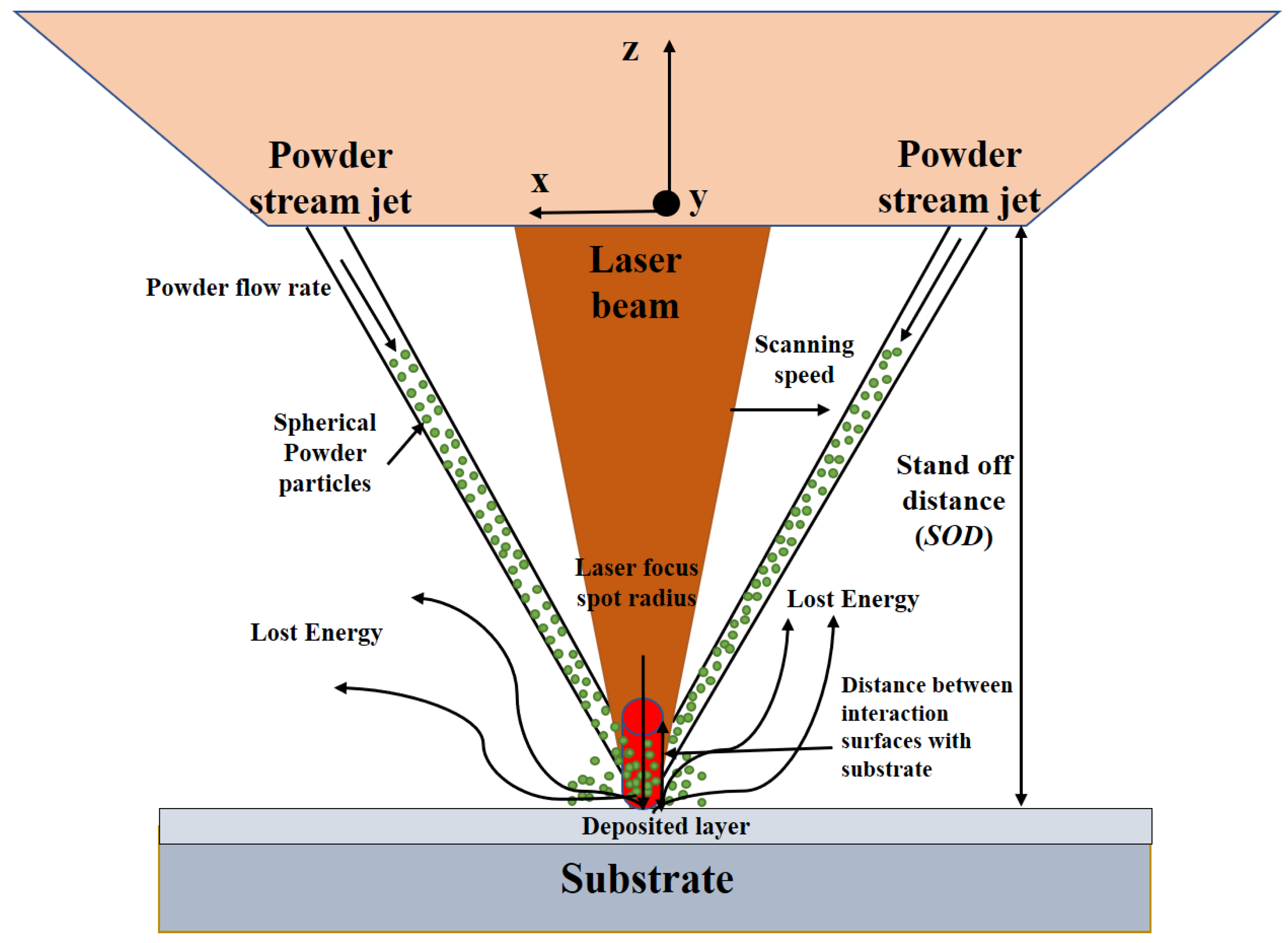
2.1. Computational Fluid Dynamics (CFD) Modelling

| Element | C | Cr | Mn | Si | P | S | Ni | N | Fe |
|---|---|---|---|---|---|---|---|---|---|
| Composition | 0.07% | 17.5–19.5% | 2.0% | 1.0% | 0.045% | 0.015% | 8.0–10.5% | 0.10% | Balance |
2.2. LMD Experiments
3. Results and Discussion
4. Conclusions
- The LMD deposition process involves the simultaneous addition of powder particles. A significant portion of the laser beam energy is utilized by the powder particles to transform their phase from solid to liquid. This, in turn, reduces the net amount of laser energy arriving at the substrate, thus yielding only the conduction-mode melt flow;
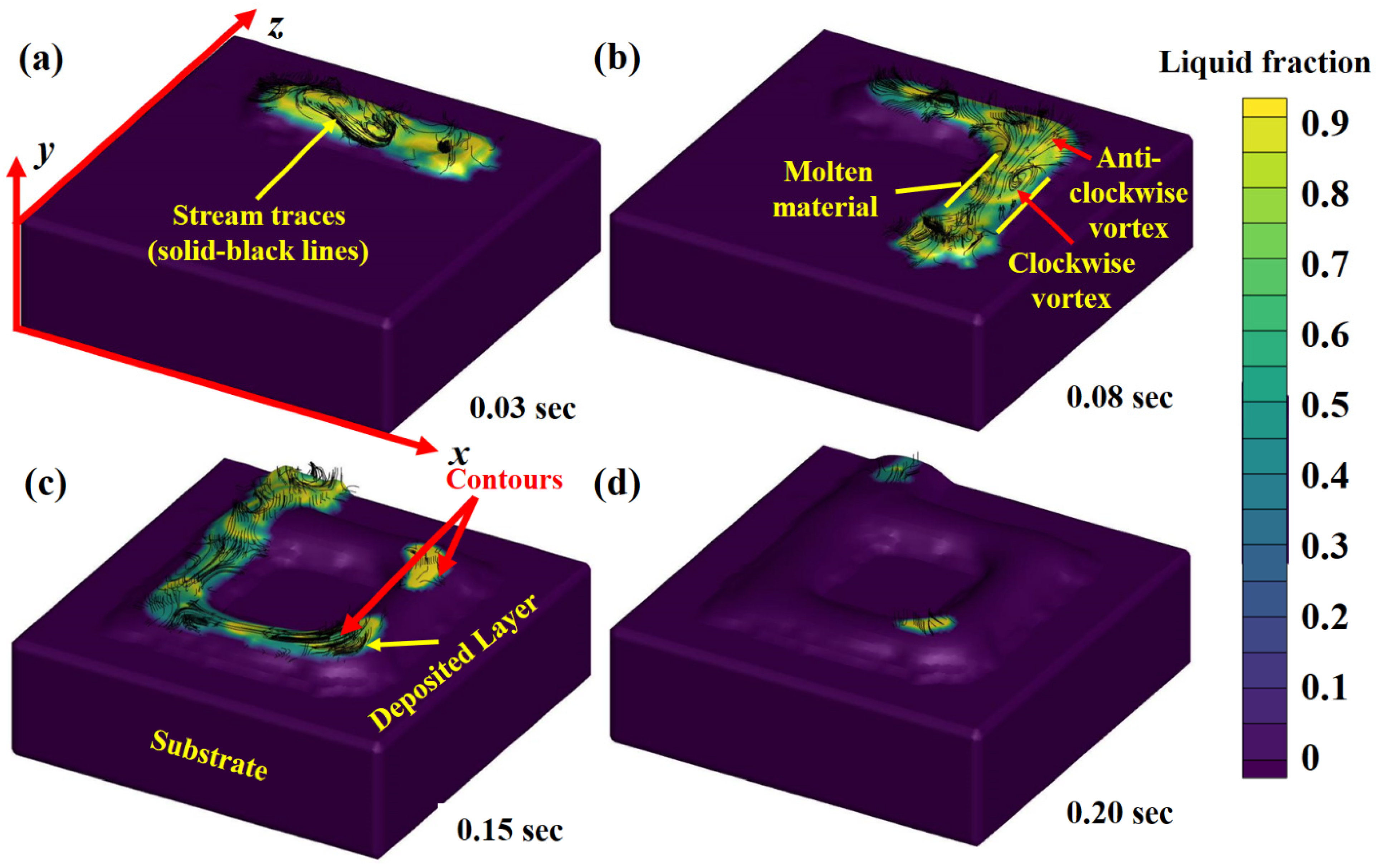
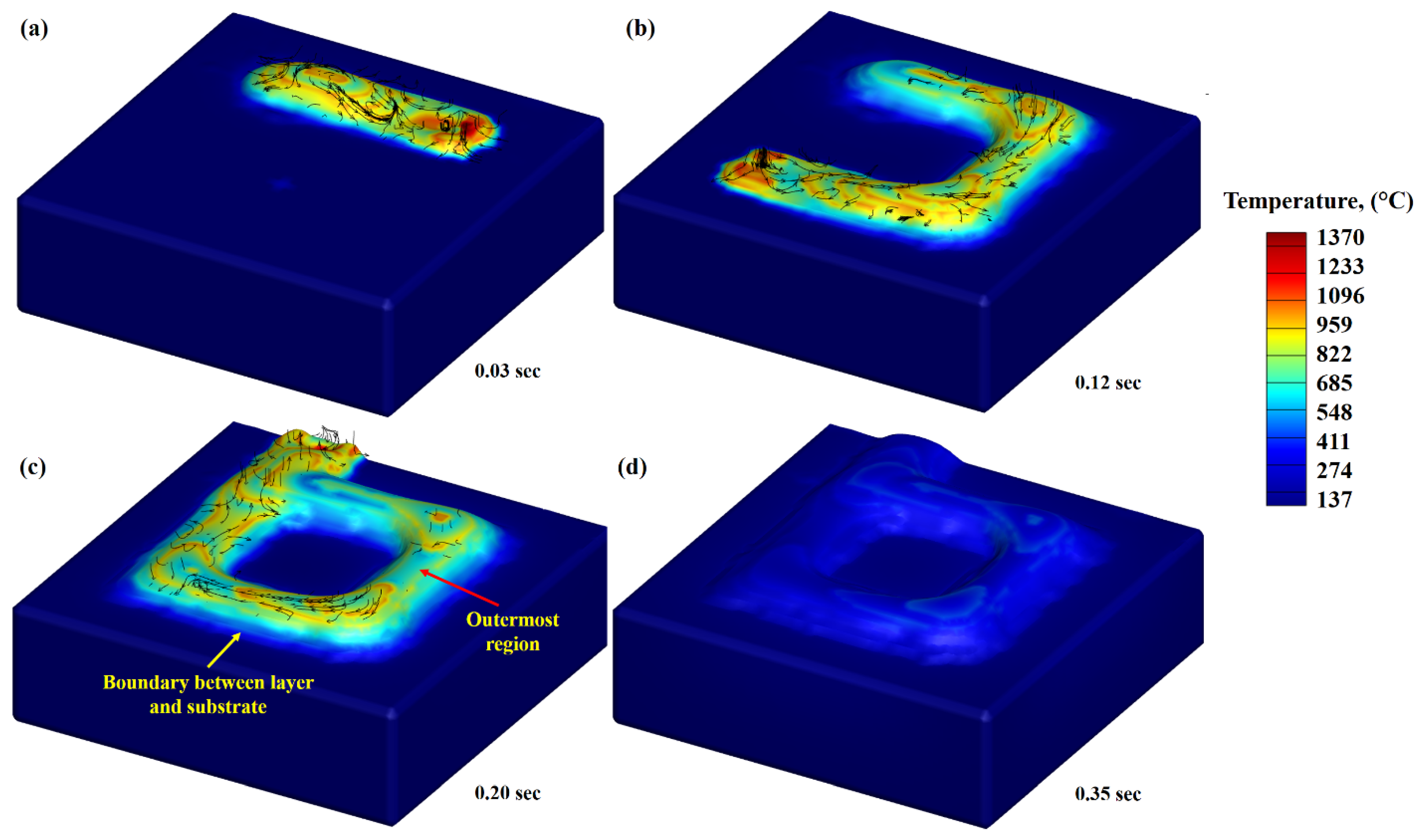
- During the deposition process, the bubbles within the melt pool float at a certain velocity and escape from the melt pool. The pores are usually entrapped within the melt pool if the solid front hits the bubble before escaping the melt pool. From simulations, it is clear that the counters of the deposited layer took the longest time to solidify compared to the entire deposition. The bubbles try to escape from the contours and become stuck during solidification, resulting in a tremendous amount of pore formation;
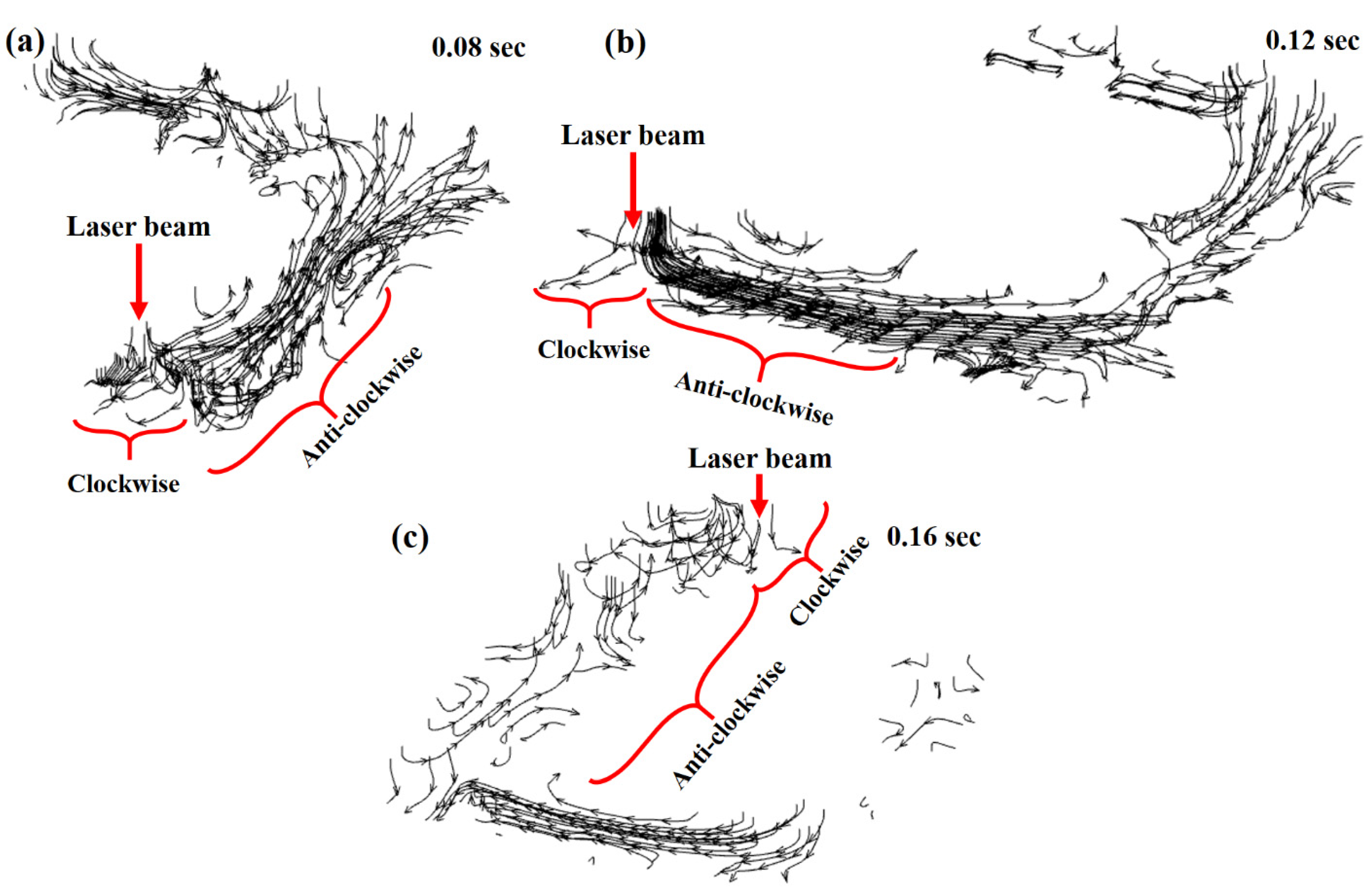
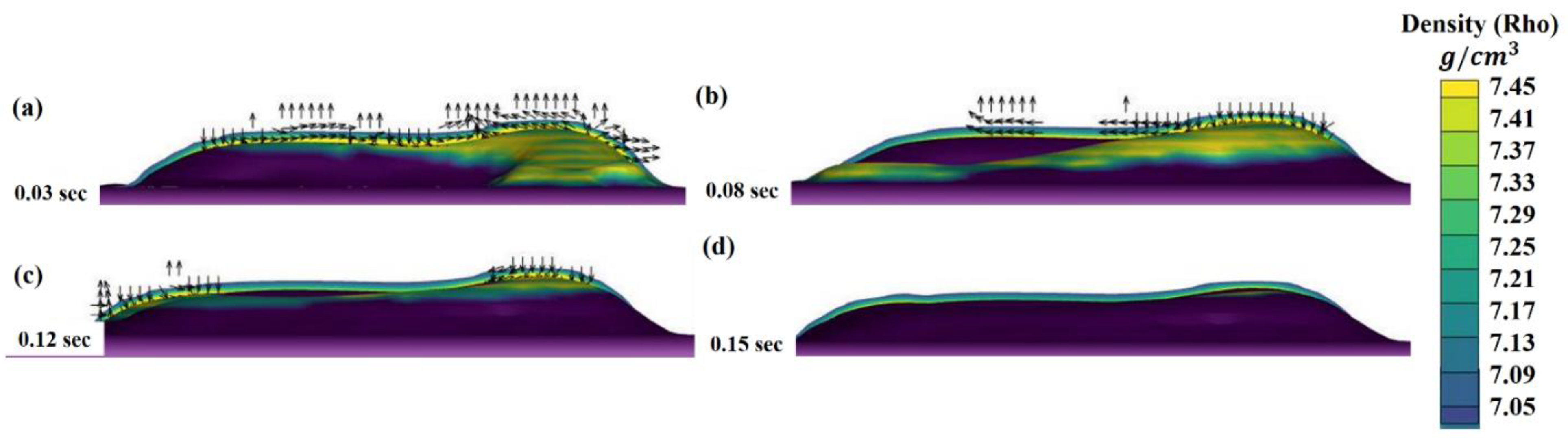
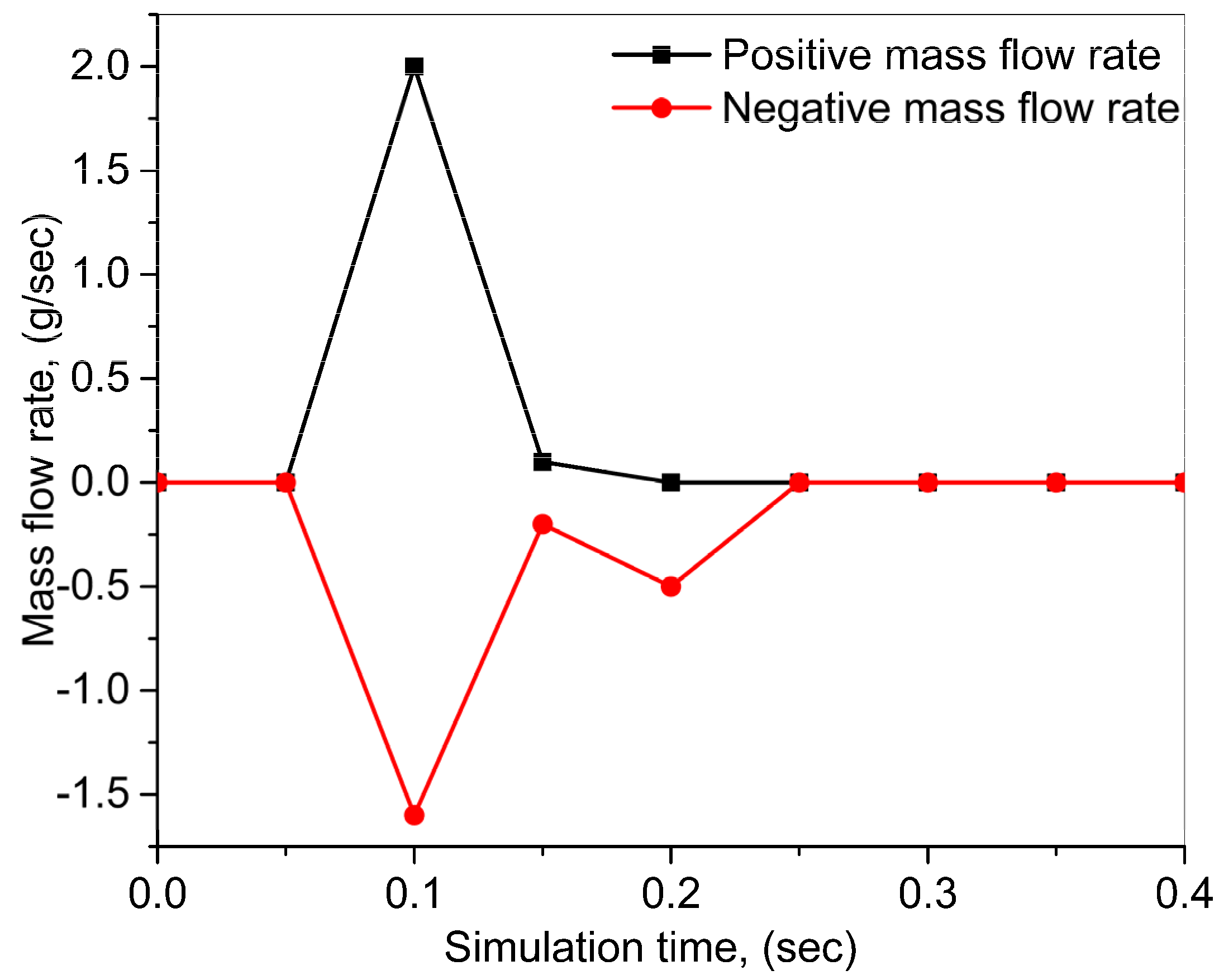
- The positive and negative mass flow rates were identified during the deposition process. The positive mass flow rate shows that the flow is going forward, while the negative shows the flow in the backward direction. When the laser beam heats the material at a specific location, the melt pool flows forward, but as the laser moves forward, the melt pool is pulled back due to the difference in the surface tension. A combination of positive and negative mass flow rates produces discontinuity in the melt pool, which disturbs the microstructural homogeneity in the deposited layer, thus affecting the final thermomechanical characteristics of the printed part. A melt pool can be classified into three regions: (a) a melt region, (b) a mushy zone, and (c) a solidified region. The mushy zone plays a critical role in defining the microstructural distribution;
- In the LMD, the “thermocapillary or Benard–Marangoni convection” is not dominant compared to the selective laser melting process. The laser beam generates a melt pool in the substrate and melts the powder particles added simultaneously, disturbing the “thermocapillary or Benard–Marangoni convection force” developed in the substrate.
Author Contributions
Funding
Data Availability Statement
Acknowledgments
Conflicts of Interest
References
- Mahmood, M.A.; Popescu, A.C.; Hapenciuc, C.L.; Ristoscu, C.; Visan, A.I.; Oane, M.; Mihailescu, I.N. Estimation of clad geometry and corresponding residual stress distribution in laser melting deposition: Analytical modeling and experimental correlations. Int. J. Adv. Manuf. Technol. 2020, 111, 77–91. [Google Scholar] [CrossRef]
- Mahmood, M.A.; Popescu, A.C.; Oane, M.; Ristoscu, C.; Chioibasu, D.; Mihai, S.; Mihailescu, I.N. Three-Jet Powder Flow and Laser–Powder Interaction in Laser Melting Deposition: Modelling Versus Experimental Correlations. Metals 2020, 10, 1113. [Google Scholar] [CrossRef]
- Daub, R. Erhöhung der Nahttiefe beim Laserstrahl-Wärmeleitungsschweißen von Stählen; Herbert Utz Verlag: München, Germany, 2012; ISBN 9783831641994. [Google Scholar]
- Zhao, C.X.; Richardson, I.M.; Pan, Y. Liquid metal flow behaviour during conduction laser spot welding. Weld. World 2009, 53, 271–275. [Google Scholar]
- Tanaka, M. An introduction to physical phenomena in arc welding processes. Weld. Int. 2004, 18, 845–851. [Google Scholar] [CrossRef]
- Kumar, A.; Roy, S. Effect of three-dimensional melt pool convection on process characteristics during laser cladding. Comput. Mater. Sci. 2009, 46, 495–506. [Google Scholar] [CrossRef]
- Han, L.; Liou, F.W.; Phatak, K.M. Modeling of laser cladding with powder injection. Metall. Mater. Trans. B 2004, 35, 1139–1150. [Google Scholar] [CrossRef]
- Gasser, A. Oberflächenbehandlung Metallischer Werkstoffe Mit CO2-Laserstrahlung in der Flüssigen Phase; Aachen Mainz: Mainz, Germany, 1993. [Google Scholar]
- Mazumder, J. Overview of melt dynamics in laser processing. Opt. Eng. 1991, 30, 1208. [Google Scholar] [CrossRef]
- Hoadley, A.F.A.; Rappaz, M. A thermal model of laser cladding by powder injection. Metall. Trans. B 1992, 23, 631–642. [Google Scholar] [CrossRef]
- Picasso, M.; Rappaz, M. Laser-powder-material interactions in the laser cladding process. J. Phys. IV Proc. 1994, 4, C4-27–C4-33. [Google Scholar] [CrossRef]
- Toyserkani, E.; Khajepour, A.; Corbin, S. 3-D finite element modeling of laser cladding by powder injection: Effects of laser pulse shaping on the process. Opt. Lasers Eng. 2004, 41, 849–867. [Google Scholar] [CrossRef]
- Choi, J.; Han, L.; Hua, Y. Modeling and Experiments of Laser Cladding With Droplet Injection. J. Heat Transf. 2005, 127, 978–986. [Google Scholar] [CrossRef]
- Wen, S.; Shin, Y.C. Modeling of transport phenomena during the coaxial laser direct deposition process. J. Appl. Phys. 2010, 108, 044908. [Google Scholar] [CrossRef]
- Sahoo, P.; Debroy, T.; McNallan, M.J. Surface tension of binary metal—surface active solute systems under conditions relevant to welding metallurgy. Metall. Trans. B 1988, 19, 483–491. [Google Scholar] [CrossRef]
- Haeri, S.; Wang, Y.; Ghita, O.; Sun, J. Discrete element simulation and experimental study of powder spreading process in additive manufacturing. Powder Technol. 2017, 306, 45–54. [Google Scholar] [CrossRef] [Green Version]
- Su, Y.; Mills, K.C.; Dinsdale, A. A model to calculate surface tension of commercial alloys. J. Mater. Sci. 2005, 40, 2185–2190. [Google Scholar] [CrossRef]
- Zhao, C.X.; Kwakernaak, C.; Pan, Y.; Richardson, I.M.; Saldi, Z.; Kenjeres, S.; Kleijn, C.R. The effect of oxygen on transitional Marangoni flow in laser spot welding. Acta Mater. 2010, 58, 6345–6357. [Google Scholar] [CrossRef]
- Cleary, P.W.; Sawley, M.L. DEM modelling of industrial granular flows: 3D case studies and the effect of particle shape on hopper discharge. Appl. Math. Model. 2002, 26, 89–111. [Google Scholar] [CrossRef]
- Parteli, E.J.R.; Pöschel, T. Particle-based simulation of powder application in additive manufacturing. Powder Technol. 2016, 288, 96–102. [Google Scholar] [CrossRef]
- Cao, L. Numerical simulation of the impact of laying powder on selective laser melting single-pass formation. Int. J. Heat Mass Transf. 2019, 141, 1036–1048. [Google Scholar] [CrossRef]
- Tian, Y.; Yang, L.; Zhao, D.; Huang, Y.; Pan, J. Numerical analysis of powder bed generation and single track forming for selective laser melting of SS316L stainless steel. J. Manuf. Process. 2020, 58, 964–974. [Google Scholar] [CrossRef]
- How to Reference FLOW-3D Products—FLOW-3D. Available online: https://www.flow3d.com/resources/bibliography/how-to-reference-flow-3d-products/ (accessed on 20 September 2021).
- Stainless Steel 304—1.4301 Data Sheet. Available online: https://www.thyssenkrupp-materials.co.uk/stainless-steel-304-14301.html (accessed on 16 March 2020).
- ASM Material Data Sheet. Available online: http://asm.matweb.com/search/SpecificMaterial.asp?bassnum=mq304a (accessed on 17 May 2020).
- Properties: Stainless Steel—Grade 304 (UNS S30400). Available online: https://www.azom.com/properties.aspx?ArticleID=965 (accessed on 17 May 2020).
- Lee, Y.S.; Zhang, W. Modeling of heat transfer, fluid flow and solidification microstructure of nickel-base superalloy fabricated by laser powder bed fusion. Addit. Manuf. 2016, 12, 178–188. [Google Scholar] [CrossRef] [Green Version]
- Guo, Q.; Zhao, C.; Qu, M.; Xiong, L.; Hojjatzadeh, S.M.H.; Escano, L.I.; Parab, N.D.; Fezzaa, K.; Sun, T.; Chen, L. In-situ full-field mapping of melt flow dynamics in laser metal additive manufacturing. Addit. Manuf. 2020, 31, 100939. [Google Scholar] [CrossRef]
- Messler, J.R.W. Principles of Welding: Processes, Physics, Chemistry, and Metallurgy; John Wiley & Sons: New York, NY, USA, 2008; ISBN 3527617493/9783527617494. [Google Scholar]
- Chioibasu, D.; Mihai, S.; Mahmood, M.A.; Lungu, M.; Porosnicu, I.; Sima, A.; Dobrea, C.; Tiseanu, I.; Popescu, A.C. Use of X-ray computed tomography for assessing defects in Ti grade 5 parts produced by laser melting deposition. Metals 2020, 10, 1408. [Google Scholar] [CrossRef]
- Yin, J.; Zhu, H.; Ke, L.; Hu, P.; He, C.; Zhang, H.; Zeng, X. A finite element model of thermal evolution in laser micro sintering. Int. J. Adv. Manuf. Technol. 2016, 83, 1847–1859. [Google Scholar] [CrossRef]
- Liu, C.; Li, C.; Zhang, Z.; Sun, S.; Zeng, M.; Wang, F.; Guo, Y.; Wang, J. Modeling of thermal behavior and microstructure evolution during laser cladding of AlSi10Mg alloys. Opt. Laser Technol. 2020, 123, 105926. [Google Scholar] [CrossRef]
- Paul, A.; Debroy, T. Free surface flow and heat transfer in conduction mode laser welding. Metall. Trans. B 1988, 19, 851–858. [Google Scholar] [CrossRef]
- Aucott, L.; Dong, H.; Mirihanage, W.; Atwood, R.; Kidess, A.; Gao, S.; Wen, S.; Marsden, J.; Feng, S.; Tong, M.; et al. Revealing internal flow behaviour in arc welding and additive manufacturing of metals. Nat. Commun. 2018, 9, 5414. [Google Scholar] [CrossRef] [PubMed] [Green Version]
- Abderrazak, K.; Bannour, S.; Mhiri, H.; Lepalec, G.; Autric, M. Numerical and experimental study of molten pool formation during continuous laser welding of AZ91 magnesium alloy. Comput. Mater. Sci. 2009, 44, 858–866. [Google Scholar] [CrossRef]
- Eriksson, I.; Powell, J.; Kaplan, A.F.H. Melt behavior on the keyhole front during high speed laser welding. Opt. Lasers Eng. 2013, 51, 735–740. [Google Scholar] [CrossRef] [Green Version]
- Nakamura, H.; Kawahito, Y.; Nishimoto, K.; Katayama, S. Elucidation of melt flows and spatter formation mechanisms during high power laser welding of pure titanium. J. Laser Appl. 2015, 27, 032012. [Google Scholar] [CrossRef]
- Matsunawa, A.; Seto, N.; Mizutani, M.; Katayama, S. Liquid motion in keyhole laser welding. Int. Congr. Appl. Lasers Electro-Opt. 1998, 1998, G151–G160. [Google Scholar] [CrossRef]
- Chang, B.; Allen, C.; Blackburn, J.; Hilton, P.; Du, D. Fluid Flow Characteristics and Porosity Behavior in Full Penetration Laser Welding of a Titanium Alloy. Metall. Mater. Trans. B 2014, 46, 906–918. [Google Scholar] [CrossRef]
- Peng, J.; Li, L.; Lin, S.; Zhang, F.; Pan, Q.; Katayama, S. High-Speed X-Ray Transmission and Numerical Study of Melt Flows inside the Molten Pool during Laser Welding of Aluminum Alloy. Math. Probl. Eng. 2016, 2016, 1409872. [Google Scholar] [CrossRef] [Green Version]
- Sohail, M.; Han, S.-W.; Na, S.-J.; Gumenyuk, A.; Rethmeier, M. Characteristics of weld pool behavior in laser welding with various power inputs. Weld. World 2014, 58, 269–277. [Google Scholar] [CrossRef]
- Cao, L.; Yuan, X. Study on the numerical simulation of the SLM molten pool dynamic behavior of a nickel-based superalloy on the workpiece scale. Materials 2019, 12, 2272. [Google Scholar] [CrossRef] [PubMed] [Green Version]


| Sample. No. | Laser Power (W) | Laser Scanning Speed (m/s) | Powder Feeding Rate (g/min) | Helium and Argon Gases (bar) | No. of Deposited Tracks | Height/Width of the Clad (mm) |
|---|---|---|---|---|---|---|
| 01 | 700 | 0.005 | 3.0 | 3.0/7.0 | 1.0 | 0.42/2.41 |
| 02 | 700 | 0.015 | 3.0 | 0.38/2.12 | ||
| 03 | 700 | 0.025 | 3.0 | 0.32/1.94 | ||
| 04 | 500 | 0.005 | 2.0 | 0.10/1.42 | ||
| 05 | 500 | 0.005 | 3.0 | 0.15/1.59 | ||
| 06 | 500 | 0.005 | 5.0 | 0.19/1.74 | ||
| 07 | 500 | 0.015 | 5.0 | 0.47/2.68 | ||
| 08 | 700 | 0.015 | 5.0 | 0.58/2.97 | ||
| 09 | 900 | 0.015 | 5.0 | 0.64/3.15 |
| Name of Step | Item Used for Processing | The Fluid Used for Sample Processing | Revolution/min | Applied Load (N) | Time |
|---|---|---|---|---|---|
| Grinding | Silicon carbide paper P320 | Water | 250 | 28 | Until plane |
| Polishing |
|
|
|
|
|
| Etching | Reagent (V2A) | N/A | N/A | N/A | 25 s |
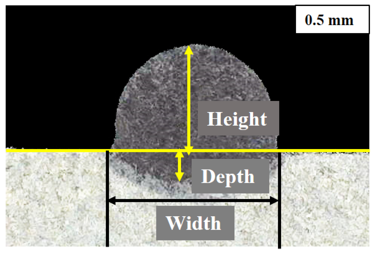
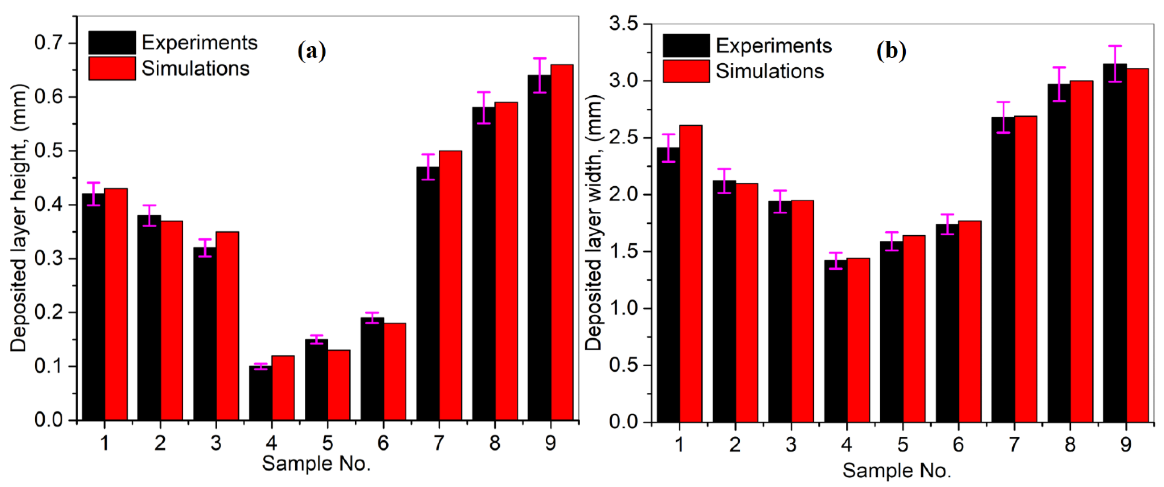
| Sample No. | Height (mm) | Width (mm) | ||
|---|---|---|---|---|
| Experiments | Simulations | Experiments | Simulations | |
| 01 | 0.42 | 0.43 | 2.41 | 2.61 |
| 02 | 0.38 | 0.37 | 2.12 | 2.1 |
| 03 | 0.32 | 0.35 | 1.94 | 1.95 |
| 04 | 0.1 | 0.12 | 1.42 | 1.44 |
| 05 | 0.15 | 0.13 | 1.59 | 1.64 |
| 06 | 0.19 | 0.18 | 1.74 | 1.77 |
| 07 | 0.47 | 0.5 | 2.68 | 2.69 |
| 08 | 0.58 | 0.59 | 2.97 | 3 |
| 09 | 0.64 | 0.66 | 3.15 | 3.11 |
Publisher’s Note: MDPI stays neutral with regard to jurisdictional claims in published maps and institutional affiliations. |
© 2021 by the authors. Licensee MDPI, Basel, Switzerland. This article is an open access article distributed under the terms and conditions of the Creative Commons Attribution (CC BY) license (https://creativecommons.org/licenses/by/4.0/).
Share and Cite
Ur Rehman, A.; Mahmood, M.A.; Pitir, F.; Salamci, M.U.; Popescu, A.C.; Mihailescu, I.N. Mesoscopic Computational Fluid Dynamics Modelling for the Laser-Melting Deposition of AISI 304 Stainless Steel Single Tracks with Experimental Correlation: A Novel Study. Metals 2021, 11, 1569. https://doi.org/10.3390/met11101569
Ur Rehman A, Mahmood MA, Pitir F, Salamci MU, Popescu AC, Mihailescu IN. Mesoscopic Computational Fluid Dynamics Modelling for the Laser-Melting Deposition of AISI 304 Stainless Steel Single Tracks with Experimental Correlation: A Novel Study. Metals. 2021; 11(10):1569. https://doi.org/10.3390/met11101569
Chicago/Turabian StyleUr Rehman, Asif, Muhammad Arif Mahmood, Fatih Pitir, Metin Uymaz Salamci, Andrei C. Popescu, and Ion N. Mihailescu. 2021. "Mesoscopic Computational Fluid Dynamics Modelling for the Laser-Melting Deposition of AISI 304 Stainless Steel Single Tracks with Experimental Correlation: A Novel Study" Metals 11, no. 10: 1569. https://doi.org/10.3390/met11101569
APA StyleUr Rehman, A., Mahmood, M. A., Pitir, F., Salamci, M. U., Popescu, A. C., & Mihailescu, I. N. (2021). Mesoscopic Computational Fluid Dynamics Modelling for the Laser-Melting Deposition of AISI 304 Stainless Steel Single Tracks with Experimental Correlation: A Novel Study. Metals, 11(10), 1569. https://doi.org/10.3390/met11101569