Fatigue Study of the Pre-Corroded 6082-T6 Aluminum Alloy in Saline Atmosphere

 ,
, 
Abstract
1. Introduction
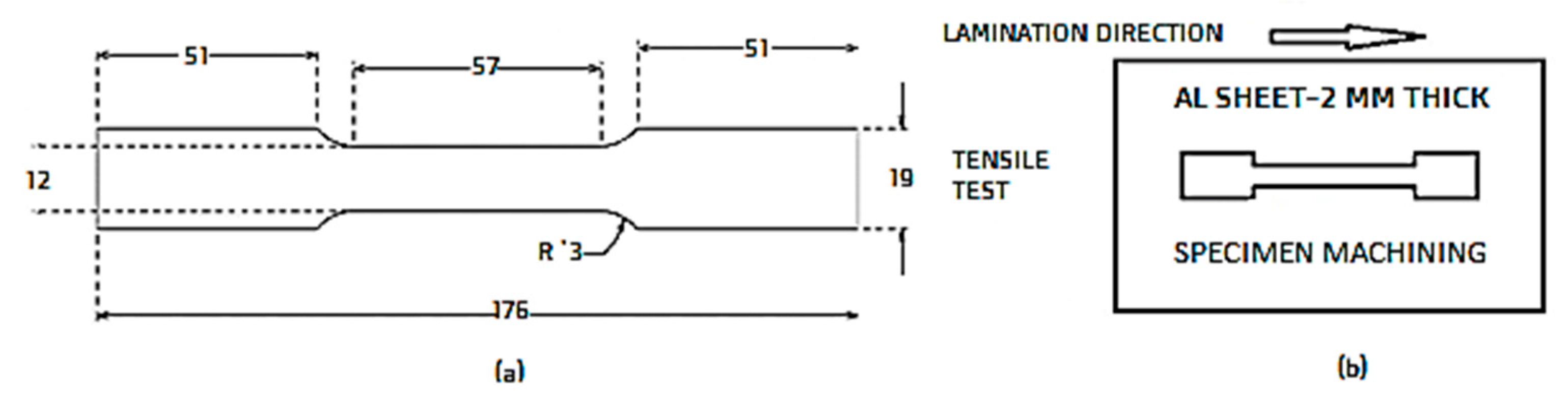
2. Materials and Methods
3. Results and Discussion
4. Conclusions
Author Contributions
Funding
Conflicts of Interest
References
- Al-Moubaraki, A.H.; Al-Rushud, H. The Red Sea as a corrosive Environment: Corrosion Rates and corrosion mechanism of aluminum alloys 7075, 2024, and 6061. Int. J. Corros. 2018, 2018, 2381287. [Google Scholar] [CrossRef]
- Mizoguchi, H.; Muraba, Y.; Fredrickson, D.C.; Matsuishi, S.; Kamiya, T.; Hosono, H. The unique electronic structure of Mg2Si: Shaping the conduction bands of semiconductors with multicenter bonding. Angew. Chem. 2017, 56, 10135–10139. [Google Scholar] [CrossRef] [PubMed]
- Kaur, K.; Ranjan, K. Electronic and thermoelectric properties of Al doped Mg2Si material: DFT study. Mater. Today Proc. 2016, 3, 1785–1791. [Google Scholar] [CrossRef]
- Couper, M.J.; Rinderer, B.; Yao, J.Y. Characterisation of AlFeSi intermetallics in 6000 series aluminium alloy extrusions. Mater. Sci. Forum 2006, 519–521, 303–308. [Google Scholar] [CrossRef]
- Prillhofer, R.; Rank, G.; Berneder, J.; Antrekowitsch, H.; Uggowitzer, P.J.; Pogatscher, S. Property criteria for automotive Al-Mg-Si sheet alloys. Materials 2014, 7, 5047–5068. [Google Scholar] [CrossRef] [PubMed]
- Linardi, E.; Haddad, R.; Lanzani, L. Stability analysis of the Mg2Si phase in AA 6061 aluminum alloy. Procedia Mater. Sci. 2012, 1, 550–557. [Google Scholar] [CrossRef]
- Zhu, M.; Zhao, B.Z.; Yuan, Y.F.; Guo, S.Y.; Pan, J. Effect of Solution Temperature on the Corrosion Behavior of 6061-T6 Aluminum Alloy in NaCl Solution. J. Mater. Eng. Perform. 2020, 29, 4725–4732. [Google Scholar] [CrossRef]
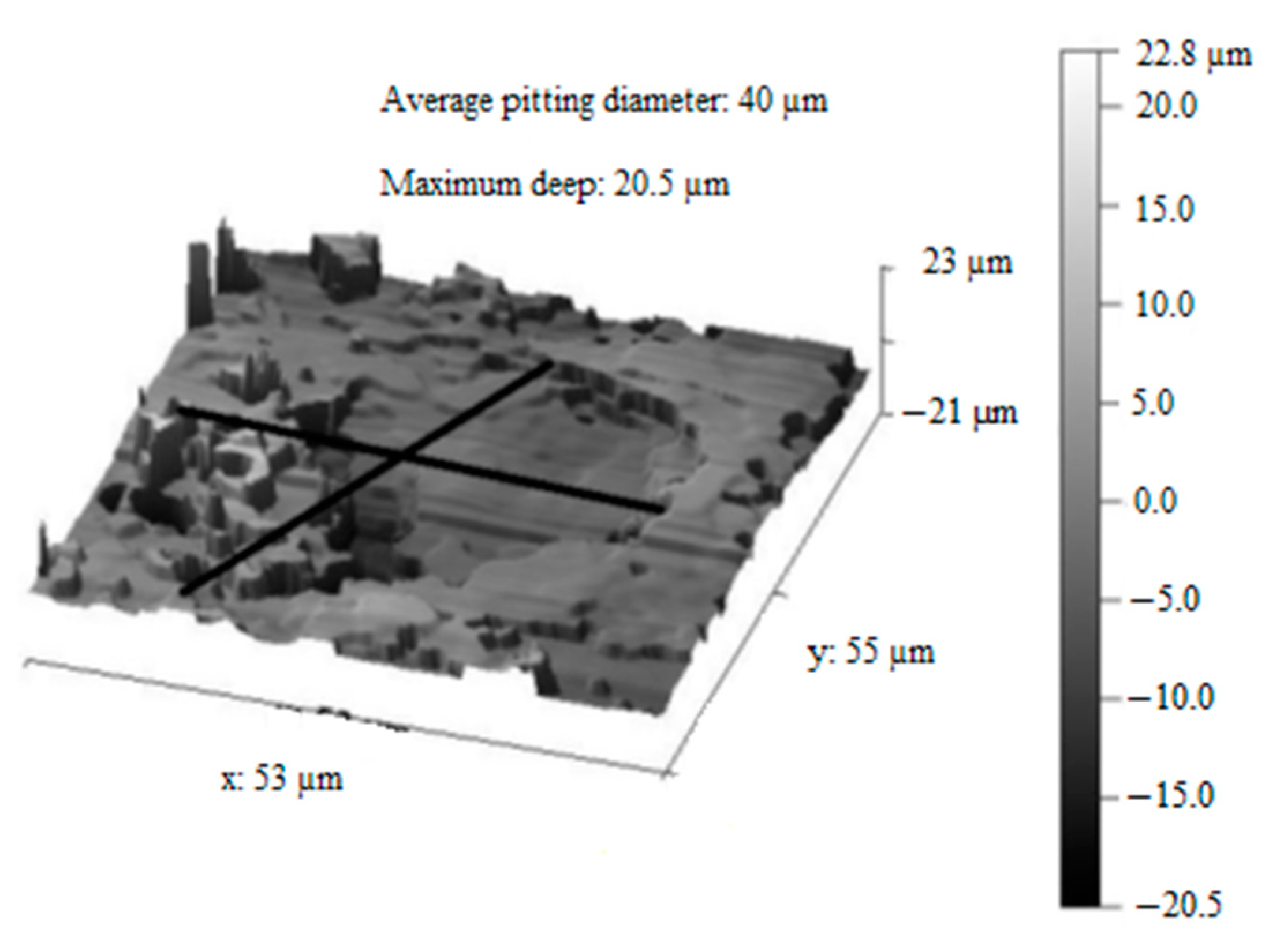
- ASTM G46-94. Standard Guide for Examination and Evaluation of Pitting Corrosion; ASTM International: West Conshohocken, PA, USA, 2018. [Google Scholar]
- McAdam, D.J., Jr. Stress-Strain-Cycle Relationship and Corrosion-Fatigue of Metals. Proc. ASTM 1926, 26, 224–280. [Google Scholar]
- Cerit, M.; Genel, K.; Eksi, S. Numerical investigation on stress concentration of corrosion pit. Eng. Fail. Anal. 2009, 16, 2467–2472. [Google Scholar] [CrossRef]
- Horner, D.A.; Connolly, B.J.; Zhou, S.; Crocker, L.; Turnbull, A. Novel images of the evolution of stress corrosion cracks from corrosion pits. Corros. Sci. 2011, 53, 3466–3485. [Google Scholar] [CrossRef]
- Yang, H.; Wang, Y.; Wang, X.; Pan, P.; Jia, D. The effects of corrosive media on fatigue performance of structural aluminum alloys. Metals 2016, 6, 160. [Google Scholar] [CrossRef]
- Sankaran, K.K.; Perez, R.; Jata, K.V. Effects of pitting corrosion on the fatigue behavior of aluminum alloy 7075-T6: Modeling and experimental studies. Mater. Sci. Eng. A 2001, 297, 223–229. [Google Scholar] [CrossRef]
- Genel, K. The effect of pitting on the bending fatigue performance of high-strength aluminum alloy. Scr. Mater. 2007, 57, 297–300. [Google Scholar] [CrossRef]
- Zupanc, U.; Grum, J. Effect of pitting corrosion on fatigue performance of shot-peened aluminium alloy 7075-T651. J. Mater. Process. Technol. 2010, 210, 1197–1202. [Google Scholar] [CrossRef]
- ASTM E8/E8M. Standard Test Methods for Tension Testing of Metallic Materials; ASTM International: West Conshohocken, PA, USA, 2008. [Google Scholar]
- ASTM B117. Standard Practice for Operating Salt Spray (Fog) Apparatus; ASTM International: West Conshohocken, PA, USA, 2019. [Google Scholar]
- Saga, M.; Kopas, P.; Uhricik, M. Modeling and experimental analysis of the aluminium alloy fatigue damage in the case of bending–torsion Loading. Procedia Eng. 2012, 48, 599–606. [Google Scholar] [CrossRef]
- Calcraft, R.C.; Schumann, G.O.; Viano, D.M. Fatigue of marine grade aluminium alloys. Aust. Weld. J. 1997, 42, 22–25. [Google Scholar]
- Gaya, A.; Lefebvre, F.; Bergamo, S.; Valiorgue, F.; Chalandond, P.; Michel, P.; Bertrand, P. Fatigue of aluminum/glass fiber reinforced polymer composite assembly joined by self-piercing riveting. Procedia Eng. 2015, 133, 501–507. [Google Scholar] [CrossRef][Green Version]
- Basquin, O.H. The exponential law of endurance tests. Am. Soc. Test. Mater. Proc. 1910, 10, 625–630. [Google Scholar]
- Ren, C.X.; Wang, D.Q.Q.; Wang, Q.; Guo, Y.S.; Zhang, Z.J.; Shao, C.W.; Yang, H.J.; Zhang, Z.F. Enhanced bending fatigue resistance of a 50CrMnMoVNb spring steel with decarburized layer by surface spinning strengthening. Int. J. Fatigue 2019, 124, 277–287. [Google Scholar] [CrossRef]
- Hong, S.; Weil, R. Low cycle fatigue of thin copper foils. Thin Solid Film. 1996, 283, 175–181. [Google Scholar] [CrossRef]
- McCool, J.I. Evaluating Weibull endurance data by the method of maximum likelihood. ASLE Trans. 1970, 13, 189–202. [Google Scholar] [CrossRef]
- Spindel, J.E.; Haibach, E. The method of maximum likelihood applied to the statistical analysis of fatigue data. Int. J. Fatigue 1979, 1, 81–88. [Google Scholar] [CrossRef]
- Marquis, G.; Mikkola, T. Analysis of welded structures with failed and non-failed welds based on maximum likelihood. Weld. World 2002, 46, 15–22. [Google Scholar] [CrossRef]
- Lorén, S.; Lundström, M. Modelling curved S-N curves. Fatigue Fract. Eng. Mater. Struct. 2005, 28, 437–443. [Google Scholar] [CrossRef]
- Myung, I.J. Tutorial on maximum likelihood estimation. J. Math. Psychol. 2003, 47, 90–100. [Google Scholar] [CrossRef]
- Setiadi, A.; Milestone, N.B.; Hill, J.; Hayes, M. Corrosion of aluminum and magnesium in BFS composite cements. Adv. Appl. Ceram. 2006, 105, 191–196. [Google Scholar] [CrossRef]
- Zhang, J.; Klasky, M.; Letellier, B.C. The aluminum chemistry and corrosion in alkaline solutions. J. Nucl. Mater. 2009, 384, 175–189. [Google Scholar] [CrossRef]
- Haidemenopoulos, G.N. Physical Metallurgy: Principles and Design; CRC Press: Boca Raton, FL, USA, 2018. [Google Scholar]
- Kun, F.; Carmona, H.; Andrade, J.S.; Herrmann, H.J. Universality behind Basquin’s Law of Fatigue. Phys. Rev. Lett. 2008, 100, 094301. [Google Scholar] [CrossRef]
- Engler-Pinto, C.C., Jr.; Lasecki, J.V.; Frisch, R.J., Sr.; Allison, J.E. Statistical approaches applied to very high cycle fatigue. In Proceedings of the Fourth International Conference on Very High Cycle Fatigue (VHCF-4), Ann Arbor, MI, USA, 19–22 August 2007; Allison, J.E., Jones, J.W., Larsen, J.M., Ritchie, R.O., Eds.; TMS (The Minerals, Metals & Materials Society): Warrendale, PA, USA, 2007; pp. 369–376. [Google Scholar]
- Jones, K.; Hoeppner, D.W. Prior corrosion and fatigue of 2024-T3 aluminum alloy. Corros. Sci. 2006, 48, 3109–3122. [Google Scholar] [CrossRef]
- Chen, G.S.; Liao, C.M.; Wan, K.C.; Gao, M.; Wei, R.P. Pitting corrosion and fatigue crack nucleation. ASTM Spec. Tech. Publ. 1997, 1298, 18–32. [Google Scholar]


| Parameter | C1 | C2 | C3 |
|---|---|---|---|
| ρp (pic/mm2) | 0.12 | 0.44 | 1.25 |
| Pmax (μm) | 39 | 57 | 130 |
| Pm (μm) | 19.5 | 26.0 | 50.0 |
| σPm | 13.2 | 14.1 | 33.0 |
| Dm (μm) | 11.5 | 10.9 | 14.1 |
| σDm | 4.5 | 5.5 | 6.8 |
| (P/D)m | 1.61 | 2.35 | 3.27 |
| Fp | 2.00 | 2.19 | 2.60 |
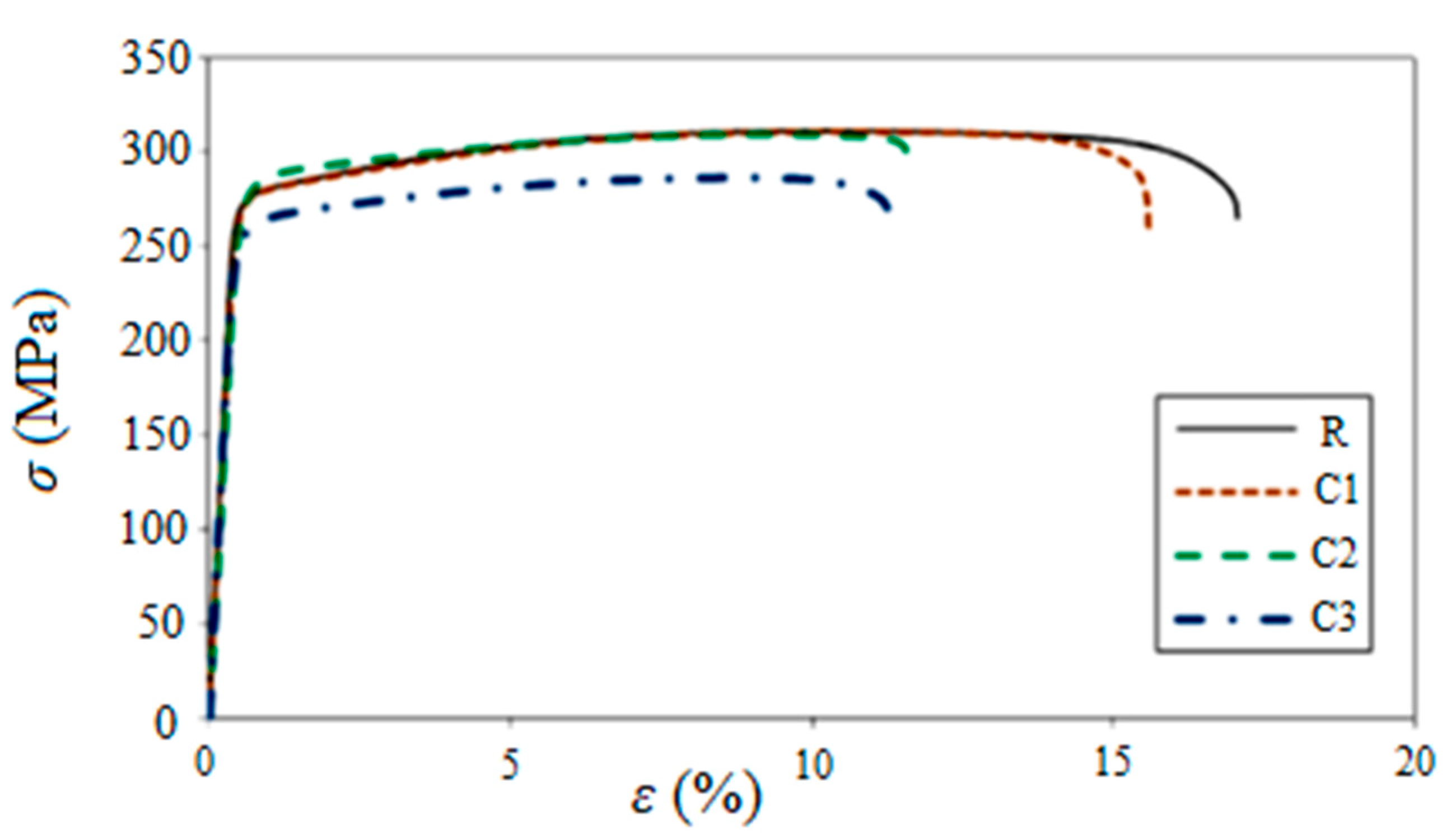
| Material | S0 (MPa) | Su (MPa) | εf |
|---|---|---|---|
| Uncorroded (R) | 275 | 311 | 17.0 |
| C1 | 271 | 311 | 15.5 |
| C2 | 276 | 309 | 11.6 |
| C3 | 255 | 286 | 11.2 |
| Sample | Smax/S0 | ΔS (MPa) | N (cycles) | σ | σ (%) |
|---|---|---|---|---|---|
| R | 0.95 | 235 | 52,432 | 20,813 | 40 |
| 0.90 | 223 | 68,404 | 29,931 | 44 | |
| 0.80 | 198 | 147,233 | 7945 | 5 | |
| 0.70 | 174 | 348,293 | 191,183 | 55 | |
| C1 | 0.95 | 235 | 20,248 | 4129 | 20 |
| 0.70 | 174 | 78,343 | 18,991 | 24 | |
| 0.55 | 136 | 175,615 | 35,238 | 20 | |
| 0.45 | 112 | 376,934 | 134,688 | 36 | |
| C2 | 0.95 | 235 | 21,944 | 2789 | 13 |
| 0.70 | 174 | 79,986 | 7991 | 10 | |
| 0.55 | 136 | 138,925 | 14,744 | 11 | |
| 0.45 | 112 | 264,567 | 23,102 | 9 | |
| C3 | 0.95 | 218 | 28,266 | 5367 | 19 |
| 0.70 | 160 | 66,757 | 15,519 | 23 | |
| 0.55 | 126 | 148,015 | 50,770 | 34 | |
| 0.45 | 103 | 236,728 | 89,123 | 38 |
| Material | K (MPa) | B | R2 |
|---|---|---|---|
| R | 1.287 | −0.1570 | 0.999 |
| C1 | 3.008 | −0.2557 | 0.996 |
| C2 | 4.846 | −0.3002 | 0.983 |
| C3 | 7.495 | −0.3453 | 0.997 |
| Material | %S0 | Smax (MPa) | F | r | Se (MPa) | σ (%) |
|---|---|---|---|---|---|---|
| R | 65 | 161 | 6 | 3 | 161 | 1.55 |
| 55 | 151 | 0 | 3 | |||
| C1 | 40 | 99 | 2 | 1 | 98 | 1.47 |
| 35 | 86 | 0 | 3 | |||
| C2 | 40 | 99 | 4 | 0 | 94 | 0.21 |
| 35 | 86 | 0 | 3 | |||
| C3 | 35 | 68 | 2 | 1 | 68 | 0.76 |
| 27 | 62 | 0 | 3 |
© 2020 by the authors. Licensee MDPI, Basel, Switzerland. This article is an open access article distributed under the terms and conditions of the Creative Commons Attribution (CC BY) license (http://creativecommons.org/licenses/by/4.0/).
Share and Cite
Muñoz, A.F.; Buenhombre, J.L.M.; García-Diez, A.I.; Fabal, C.C.; Díaz, J.J.G. Fatigue Study of the Pre-Corroded 6082-T6 Aluminum Alloy in Saline Atmosphere. Metals 2020, 10, 1260. https://doi.org/10.3390/met10091260
Muñoz AF, Buenhombre JLM, García-Diez AI, Fabal CC, Díaz JJG. Fatigue Study of the Pre-Corroded 6082-T6 Aluminum Alloy in Saline Atmosphere. Metals. 2020; 10(9):1260. https://doi.org/10.3390/met10091260
Chicago/Turabian StyleMuñoz, Alejandro Fernández, José Luis Mier Buenhombre, Ana Isabel García-Diez, Carolina Camba Fabal, and Juan José Galán Díaz. 2020. "Fatigue Study of the Pre-Corroded 6082-T6 Aluminum Alloy in Saline Atmosphere" Metals 10, no. 9: 1260. https://doi.org/10.3390/met10091260
APA StyleMuñoz, A. F., Buenhombre, J. L. M., García-Diez, A. I., Fabal, C. C., & Díaz, J. J. G. (2020). Fatigue Study of the Pre-Corroded 6082-T6 Aluminum Alloy in Saline Atmosphere. Metals, 10(9), 1260. https://doi.org/10.3390/met10091260