Development of an Instrumented Test Tool for the Determination of Heat Transfer Coefficients for Die Casting Applications


Abstract
1. Introduction
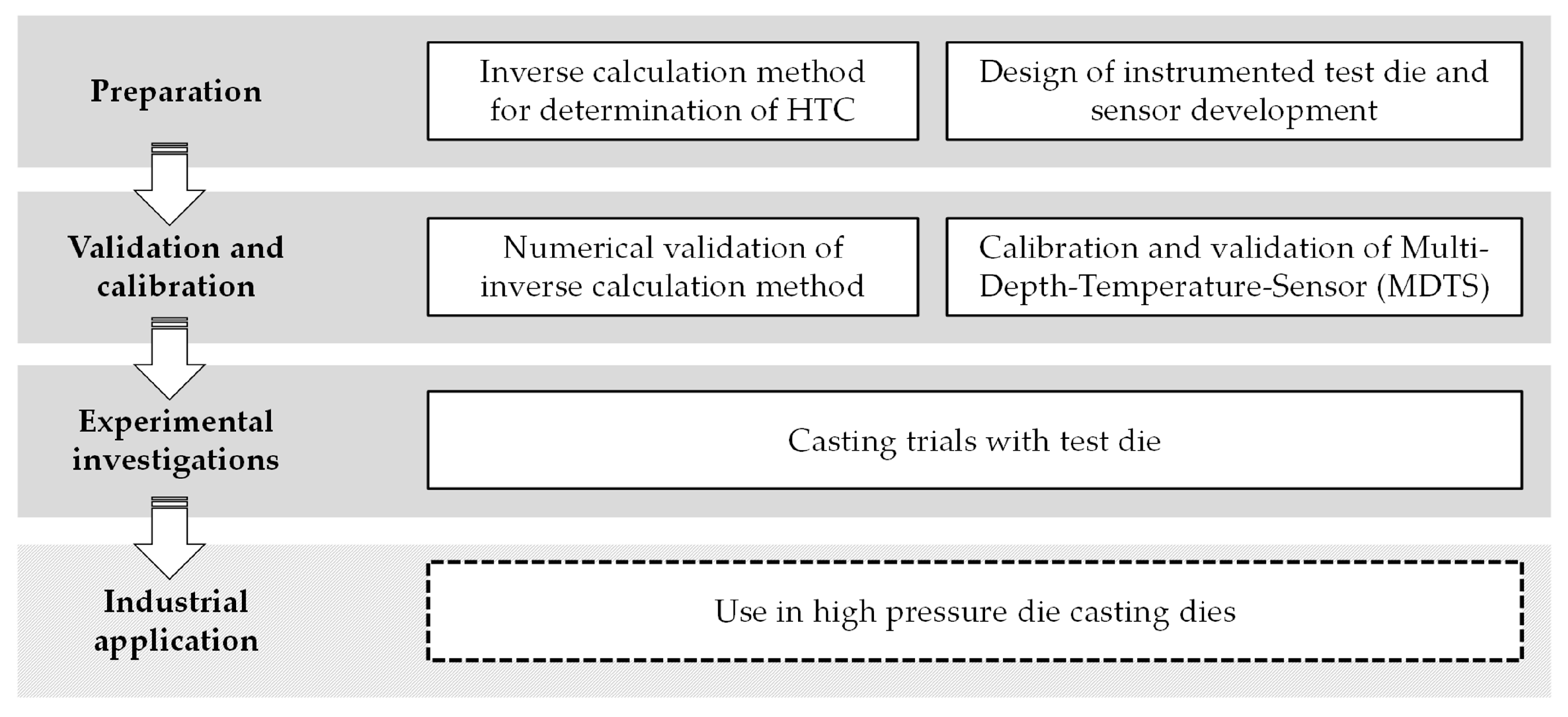
2. Methodology
3. Steps Realization
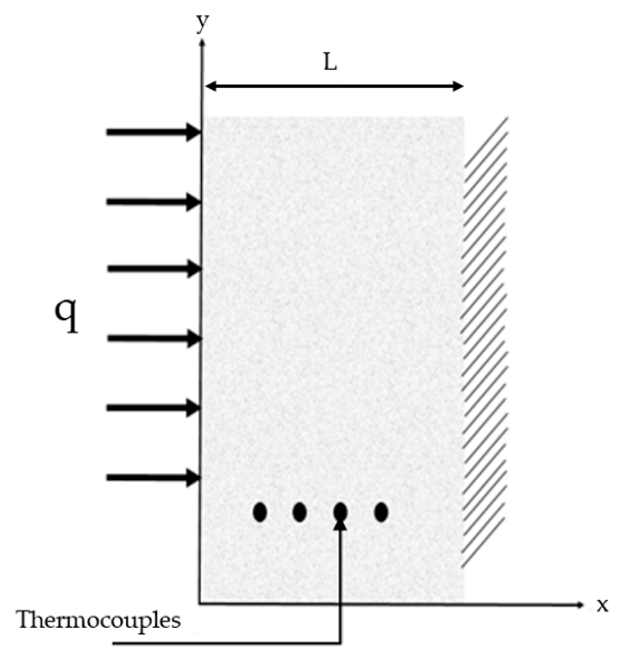
3.1. Inverse Heat Conduction Problem and Estimation of the HTC
- The initial temperature of the slab is considered to be a uniform value:
- At the surface, the slab is subjected to a transient heat flux and the temperature is suddenly changed:
- The opposite surface of the slab is insulated:
- The temperature inside the slab can be given by:where is the experimental measured temperature data. To solve the problem, minimization by the method of least squares is widely used in order to determine the surface temperature T by means of the measured temperatures Y at different locations within the body as follows:where n represents the number of observations and l represents the number of sensors or the positions of the thermocouples. The index i corresponds to the time step index and j to the position index. On this basis many inverse techniques were developed, such as the Tikhonov regularization [17]. A very efficient method, however, has been used in particular to solve nonlinear heat conduction problems and has been applied to the die casting process by many researchers [10,14,16,17,18]. This is the method of nonlinear function specification (FSM), known as Beck’s method. The FSM is sequential in nature and calculates the heat flux density function by estimating a discrete segment, starting with an initial estimate of q [19]. It also has the advantage of using a very small computational time step for more precision in the calculation. The estimated quantity of q on each small segment should be constant for a certain future time step designed by r [19]. The final solution for determining the heat flux density function q is therefore represented by Equation (3), where M is the current time step.
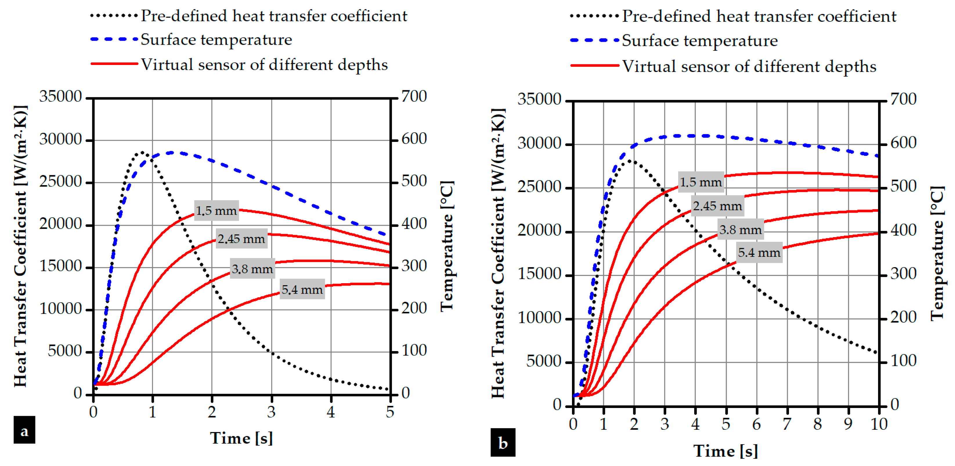
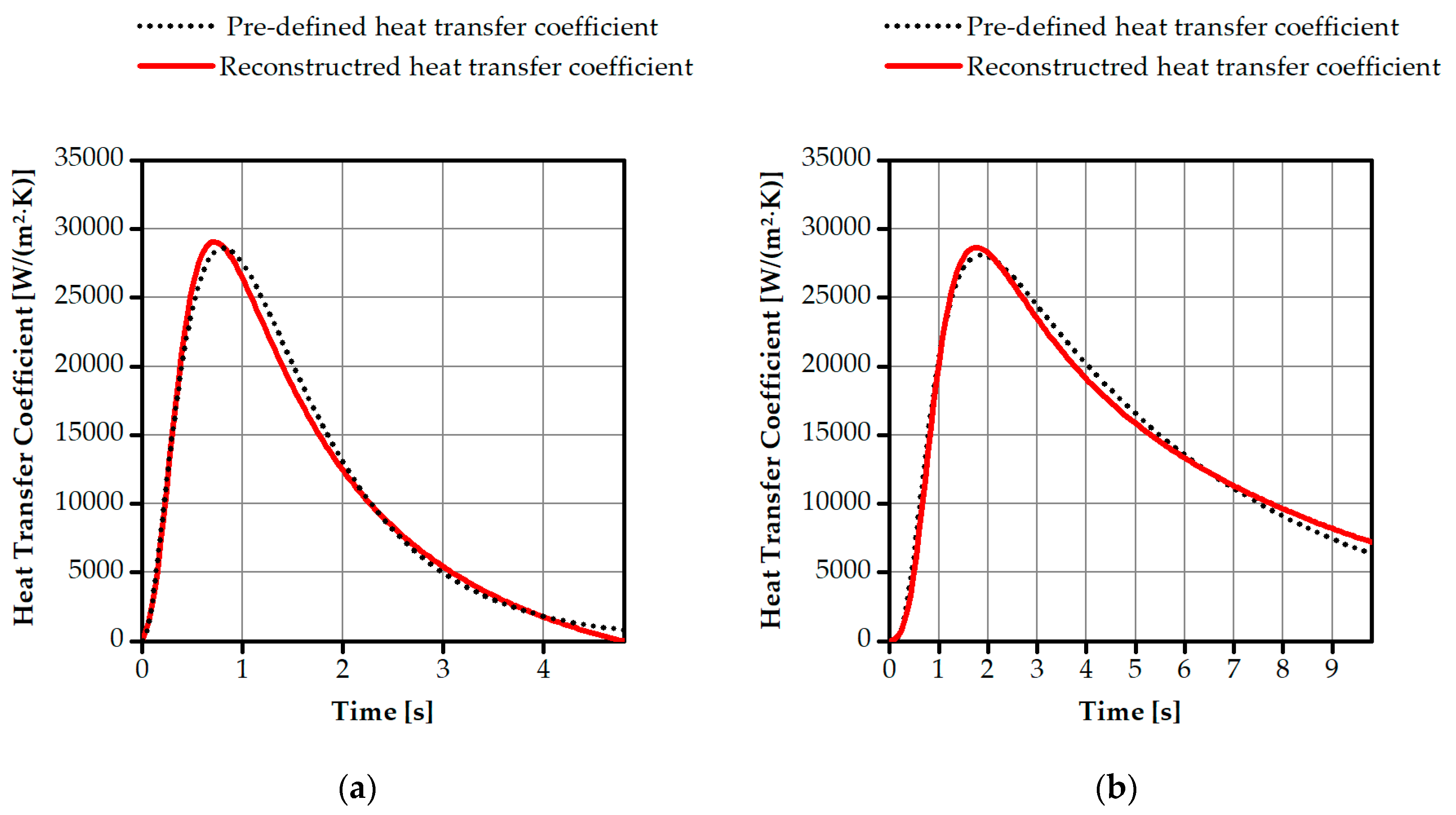
3.2. Validation of the Method
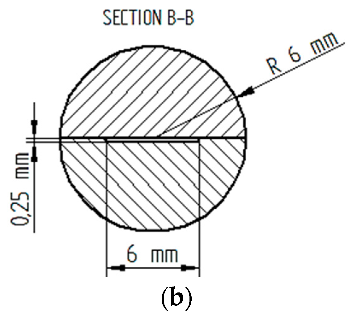
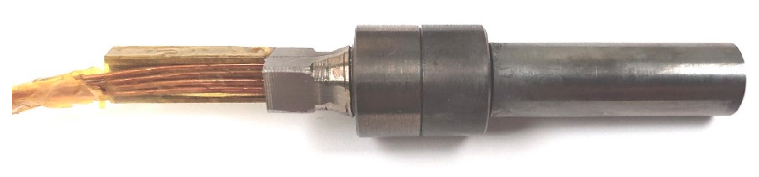
3.3. Sensor Manufacturing
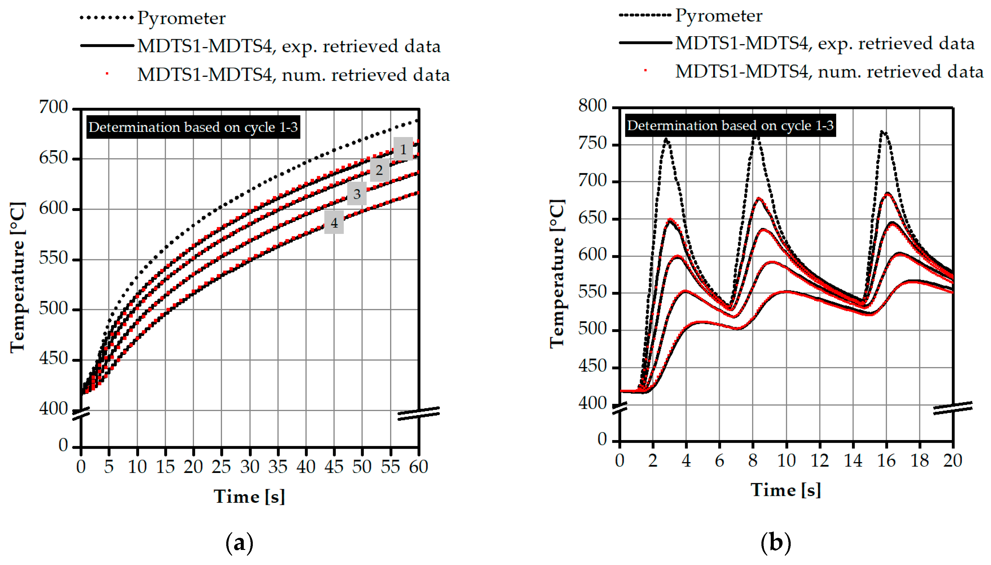
3.4. Sensor Validation
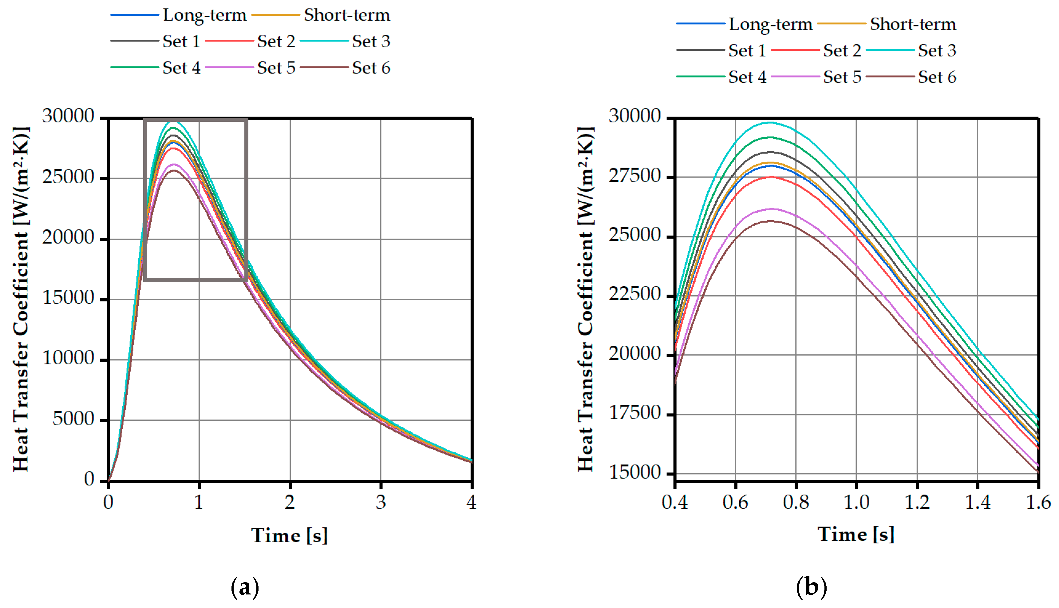
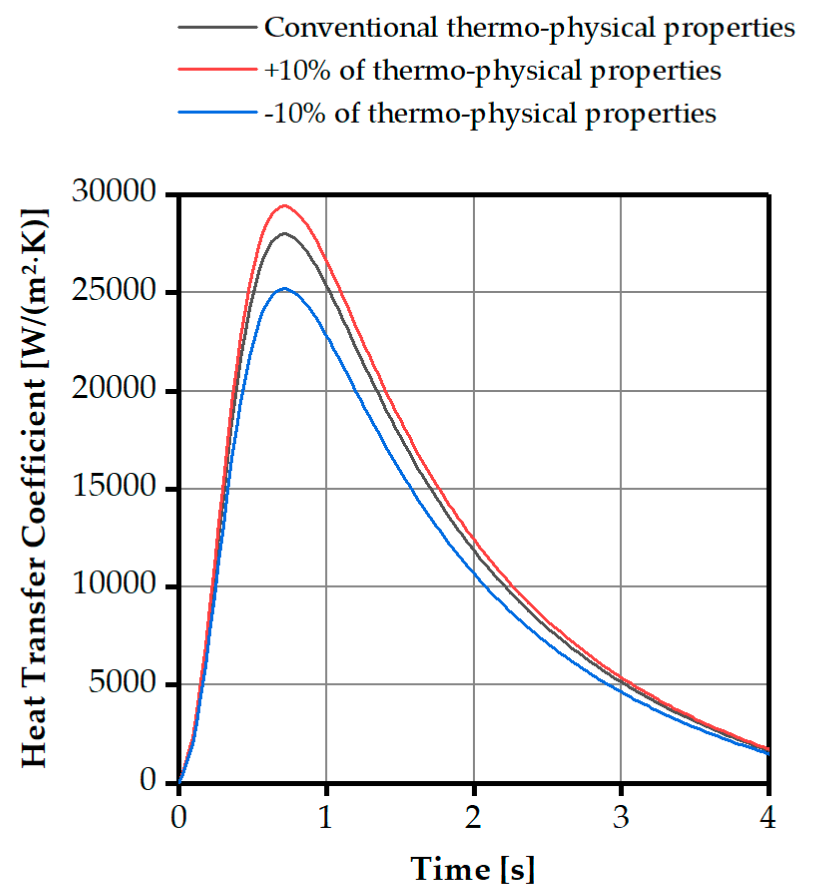
3.5. Evaluation of the Uncertainty of the HTC Reconstruction
3.6. Design of the Instrumented Test Tool
4. Experimental Results and Discussion
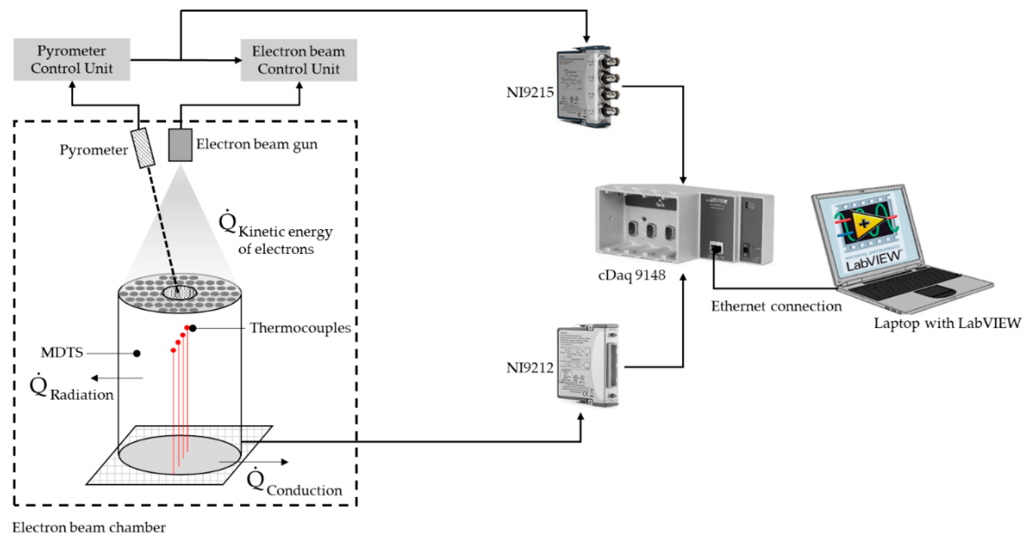
4.1. Experimental Conditions and Setup
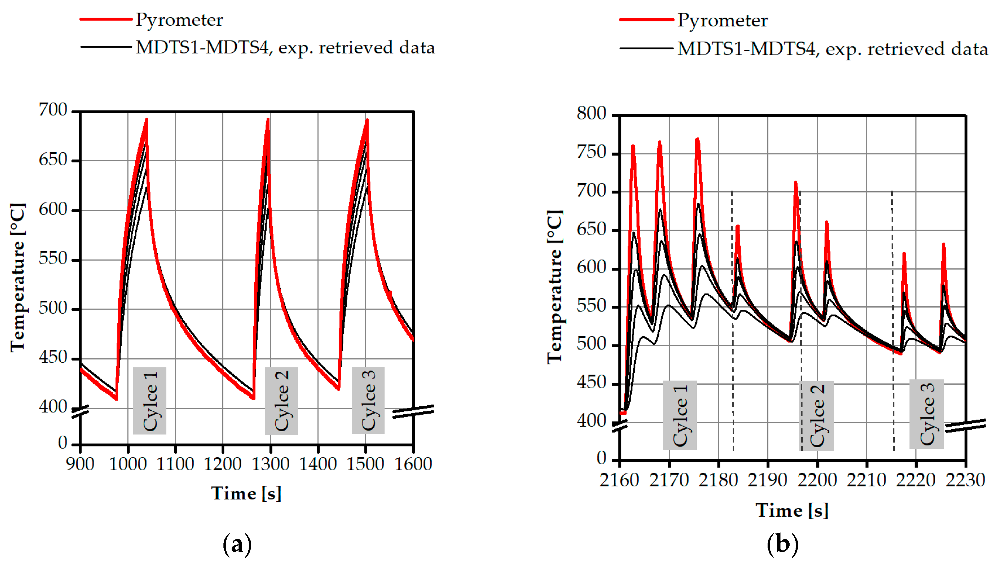
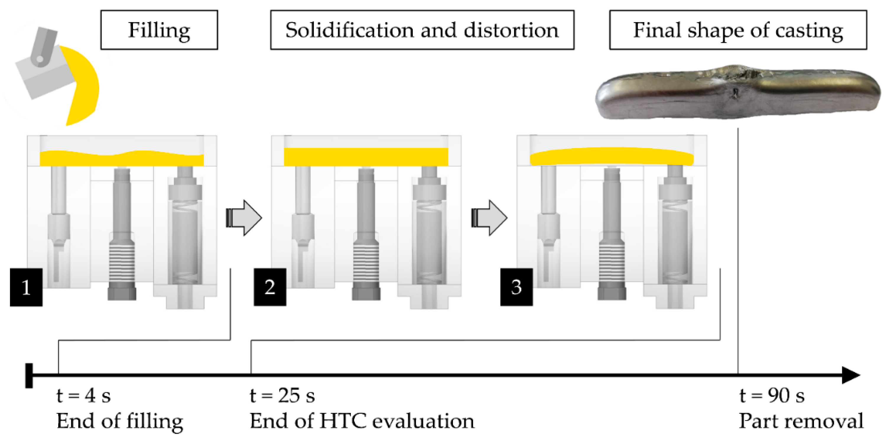
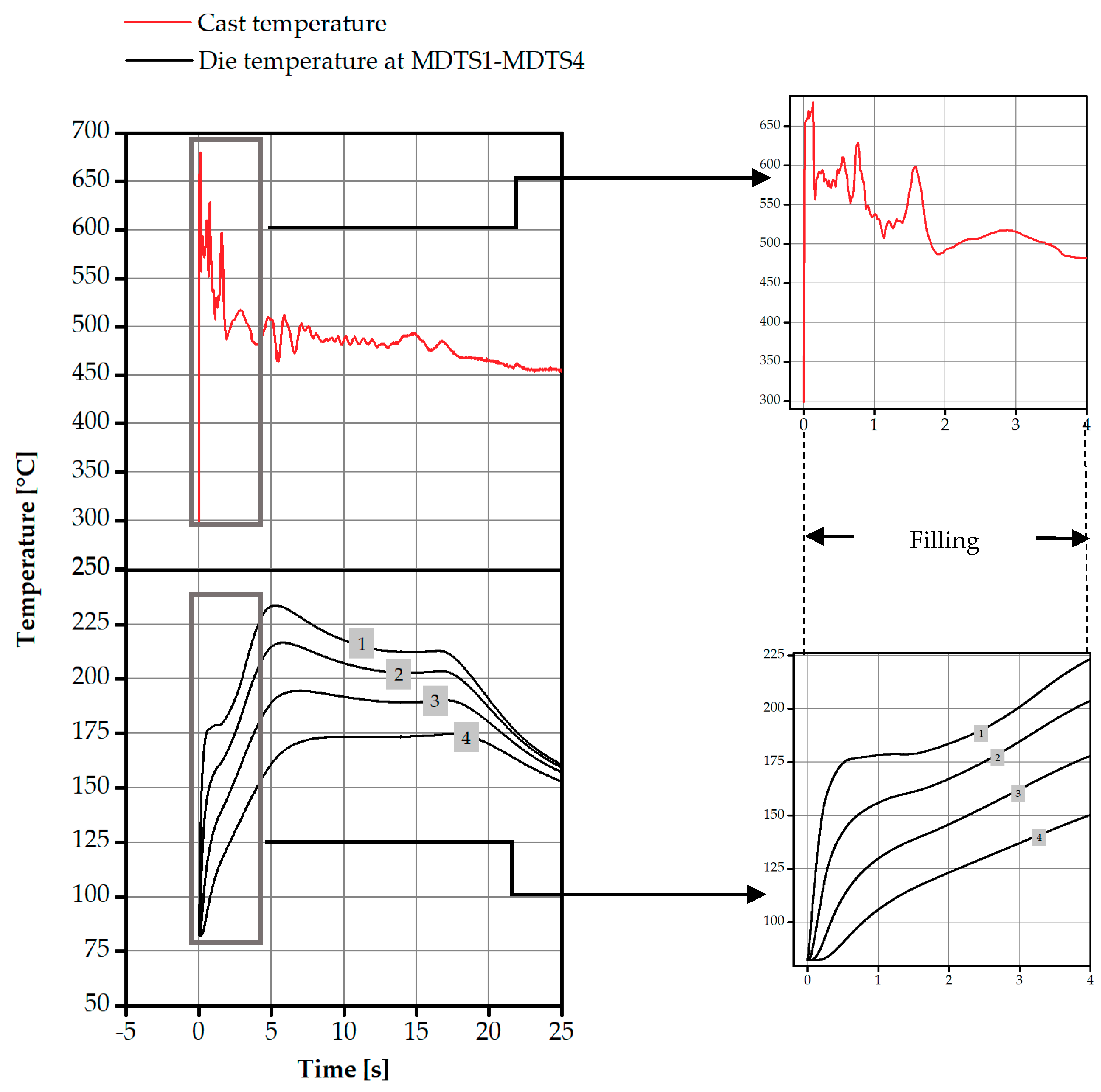
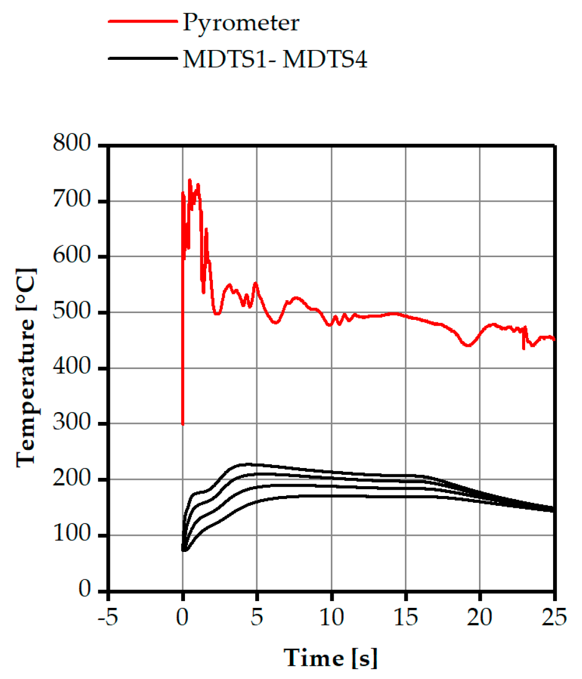
4.2. Process Description and Results
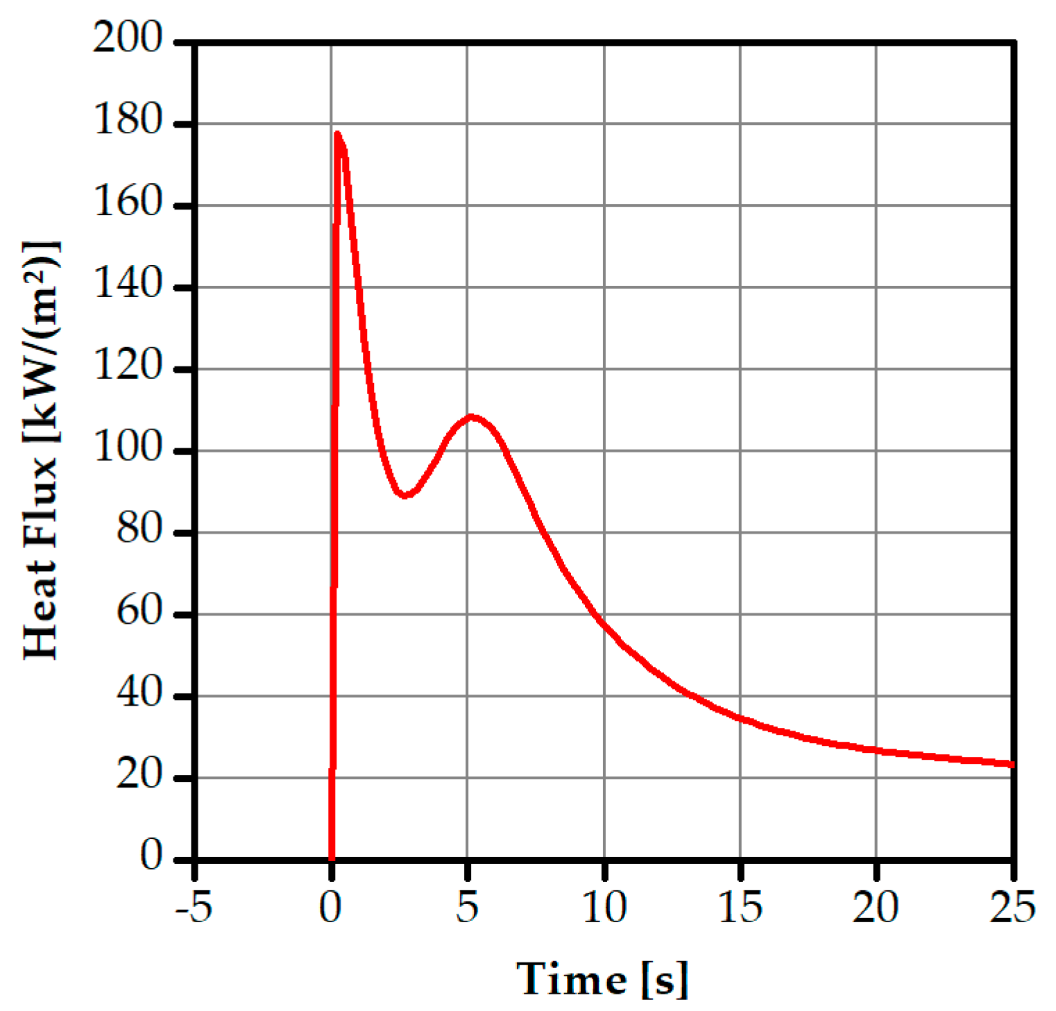
4.3. Determination of the HTC
5. Conclusions and Outlook
Author Contributions
Funding
Conflicts of Interest
Appendix A

| Long-Term Determination | Short-Term Determination | Mean Value | Standard Deviation |
|---|---|---|---|
| −1.5 | −1.5 | −1.5 | 0 |
| −2.45 | −2.5 | −2.475 | 0.03536 |
| −3.8 | −3.95 | −3.875 | 0.10607 |
| −5.4 | −5.8 | −5.6 | 0.28284 |
| Temperature (°C) | Cp (J·kg−1·K−1) | λ (W·m−1·K−1) | ρ (kg·m−3) |
|---|---|---|---|
| 20 | 440.9 | 26.5 | 7800 |
| 100 | 466.1 | 27.3 | 7776 |
| 200 | 490.9 | 28.2 | 7746 |
| 300 | 511 | 28.7 | 7716 |
| 400 | 529.2 | 29 | 7687 |
| 500 | 548.5 | 28.9 | 7645 |
| 600 | 582.3 | 28.4 | 7600 |
| 700 | 622.8 | 28.2 | 7550 |
| Element | Al | Si | Fe | Cu | Mn | Mg | Ni | Zn | Pb | Sn | Ti |
|---|---|---|---|---|---|---|---|---|---|---|---|
| Percentage | Balance | 9–11 | 0.055 | 0.1 | 0.45 | 0.20–0.45 | 0.05 | 0.10 | 0.05 | 0.05 | 0.15 |


References
- Winkler, M.; Kallien, L.; Feyertag, T. Correlation between process parameters and quality characteristics in aluminum high pressure die casting. NADCA. Available online: https://www.researchgate.net/publication/283726141_Correlation_between_process_parameters_and_quality_characteristics_in_aluminum_high_pressure_die_casting (accessed on 1 September 2020).
- Dour, G.; Dargusch, M.; Davidson, C. Recommendations and guidelines for the performance of accurate heat transfer measurements in rapid forming processes. Int. J. Heat Mass Transf. 2006, 49, 379–390. [Google Scholar] [CrossRef]
- Kobliska, J.; Ostojic, P.; Cheng, X.; Zhang, X.; Choi, H.; Yang, Y.; Li, X. Rapid Fabrication of Smart Tooling with Embedded Sensors by Casting in Molds Made by Three Dimensional Printing. Int. Solid Free. Fabr. Symp. 2005, 42, 468–475. [Google Scholar]
- Tiedemann, R.; Pille, C.; Dumstorff, G.; Lang, W. Sensor Integration in Castings Made of Aluminum—New Approaches for Direct Sensor Integration in Aluminum High Pressure Die Casting. Key Eng. Mater. 2017, 742, 786–792. [Google Scholar] [CrossRef]
- Ageyeva, T.; Horváth, S.; Kovács, J.G. In-Mold Sensors for Injection Molding: On the Way to Industry 4.0. Sensors 2019, 19, 3551. [Google Scholar] [CrossRef] [PubMed]
- Tian, L.; Guo, Y.; Li, J.; Xia, F.; Liang, M.; Bai, Y. Effects of Solidification Cooling Rate on the Microstructure and Mechanical Properties of a Cast Al-Si-Cu-Mg-Ni Piston Alloy. Materials 2018, 11, 1230. [Google Scholar] [CrossRef] [PubMed]
- Snopiński, P.; Król, M.; Tański, T.; Krupińska, B. Effect of cooling rate on microstructural development in alloy ALMG9. J. Therm. Anal. Calorim. 2018, 133, 379–390. [Google Scholar] [CrossRef]
- Hosseini, V.A.; Shabestari, S.G.; Gholizadeh, R. Study on the effect of cooling rate on the solidification parameters, microstructure, and mechanical properties of LM13 alloy using cooling curve thermal analysis technique. Mater. Des. 2013, 50, 7–14. [Google Scholar] [CrossRef]
- Jamaly, N.; Haghdadi, N.; Phillion, A.B. Microstructure, Macrosegregation, and Thermal Analysis of Direct Chill Cast AA5182 Aluminum Alloy. J. Mater. Eng. Perform. 2015, 24, 2067–2073. [Google Scholar] [CrossRef]
- Yongyou, C.; Zhipeng, G.; Shoumei, X. Determination of the metal/die interfacial heat transfer coefficient of high pressure die cast B390 alloy. IOP Conf. Ser. Mater. Sci. Eng. 2012, 33, 012010. [Google Scholar]
- Hamasaiid, A.; Dargusch, M.S.; Davidson, C.; Loulou, T.; Dour, G. A Model to Predict the Heat Transfer Coefficient at the Casting-Die Interface for the High Pressure Die Casting Process. AIP Conf. Proc. 2008, 907, 1211. [Google Scholar]
- Vasileiou, A.N.; Vosniakos, G.-C.; Pantelis, D. Determination of local heat transfer coefficients in precision castings by genetic optimisation aided by numerical simulation. Proc. IMechE Part C J. Mech. Eng. Sci. 2015, 229, 735–750. [Google Scholar] [CrossRef]
- Aksoy, B.; Koru, M. Estimation of Casting Mold Interfacial Heat Transfer Coefficient in Pressure Die Casting Process by Artificial Intelligence Methods. Arab. J. Sci. Eng. 2020, 31, 45. [Google Scholar] [CrossRef]
- Cao, Y.; Guo, Z.; Xiong, S. Determination of interfacial heat transfer coefficient and its application in high pressure die casting process. China Foundry 2014, 11, 9. [Google Scholar]
- Pille, C. Smart systems integration. In Proceedings of the 4th European Conference & Exhibition on Integration Issues of Miniaturized Systems-MEMS, MOEMS, ICs and Electronic Components, CD-ROM, Como, Italy, 23–24 March 2010. [Google Scholar]
- Zhang, Y.; Wen, Z.; Zhao, Z.; Bi, C.; Guo, Y.; Huang, J. Laboratory Experimental Setup and Research on Heat Transfer Characteristics during Secondary Cooling in Continuous Casting. Metals 2019, 9, 61. [Google Scholar] [CrossRef]
- Dhodare, A.; Ravanan, P.M.; Dodiya, N. A Review on Interfacial Heat Transfer Coefficient during Solidification in Casting. IJERT 2017, 6, 464–467. [Google Scholar]
- Dargusch, M.S.; Hamasaiid, A.; Dour, G. An Inverse Model to determine the Heat Transfer Coefficient and its Evolution with Time during Solidification of Light Alloys. Int. J. Nonlinear Sci. Numer. Simul. 2008, 9, 275–282. [Google Scholar] [CrossRef][Green Version]
- Beck, J.V. Nonlinear estimation applied to the nonlinear inverse heat conduction problem. Int. J. Heat Mass Transf. 1970, 13, 703–716. [Google Scholar] [CrossRef]
- Kaschnitz, E.; Hofer, P.; Funk, W. Thermophysikalische Daten eines Warmarbeitsstahls mit hoher Wärmeleitfähigkeit. Giesserei 2010, 97, 42–45. [Google Scholar]
- OMEGA. Available online: www.omega.de (accessed on 1 September 2020).
- Edmund Optics. Available online: https://www.edmundoptics.com/p/125mm-diameter-uncoated-sapphire-window/34724/ (accessed on 1 September 2020).
- Advanced Energy. Impac ISR 12-LO and IGAR 12-LO Series. Available online: https://www.advancedenergy.com/ (accessed on 1 September 2020).


| Evaluation Sets | Thermocouples Depths | |||
|---|---|---|---|---|
| MDTS1 | MDTS2 | MDTS3 | MDTS4 | |
| Long-term | −1.5 | −2.45 | −3.8 | −5.4 |
| Set 1 | −1.5 − 0.5 | −2.45 − 0.5 | −3.8 − 0.5 | −5.4 − 0.5 |
| Set 2 | −1.5 + 0.5 | −2.45 + 0.5 | −3.8 +0.5 | −5.4 + 0.5 |
| Set 3 | −1.5 × 1.5 | −2.45 × 1.5 | −3.8 × 1.5 | −5.4 × 1.5 |
| Set 4 | −3 | −4 | −5 | −6 |
| Set 5 | −0.5 | −1 | −1.5 | −2 |
| Set 6 | −0.25 | −0.5 | −0.75 | −1 |
© 2020 by the authors. Licensee MDPI, Basel, Switzerland. This article is an open access article distributed under the terms and conditions of the Creative Commons Attribution (CC BY) license (http://creativecommons.org/licenses/by/4.0/).
Share and Cite
Kouki, Y.; Müller, S.; Schuchardt, T.; Dilger, K. Development of an Instrumented Test Tool for the Determination of Heat Transfer Coefficients for Die Casting Applications. Metals 2020, 10, 1206. https://doi.org/10.3390/met10091206
Kouki Y, Müller S, Schuchardt T, Dilger K. Development of an Instrumented Test Tool for the Determination of Heat Transfer Coefficients for Die Casting Applications. Metals. 2020; 10(9):1206. https://doi.org/10.3390/met10091206
Chicago/Turabian StyleKouki, Yosra, Sebastian Müller, Torsten Schuchardt, and Klaus Dilger. 2020. "Development of an Instrumented Test Tool for the Determination of Heat Transfer Coefficients for Die Casting Applications" Metals 10, no. 9: 1206. https://doi.org/10.3390/met10091206
APA StyleKouki, Y., Müller, S., Schuchardt, T., & Dilger, K. (2020). Development of an Instrumented Test Tool for the Determination of Heat Transfer Coefficients for Die Casting Applications. Metals, 10(9), 1206. https://doi.org/10.3390/met10091206