Charge Plan Model for Steelmaking-Continuous Casting Section


Abstract
:1. Introduction
2. Development of a Charge Plan Model for SM-CC
2.1. Problem Description
2.2. Charge Plan Model
- (1)
- Application conditions
- (2)
- Symbol definition
- (3)
- Mathematical model
3. Process of Solving the Charge Plan Model for SM-CC
- (1)
- Read the basic data of the preselected contract pool, including the contract number, weight, steel grade, and delivery time.
- (2)
- Initialize algorithm parameters, including the iteration time, population size, crossover probability, and conventional mutation probability.
- (3)
- Initialize the population of N individuals according to the permutation coding rule.
- (4)
- Decode the chromosomes of the population.
- (5)
- Calculate the objective function values of the current populations and record the optimal individuals and their chromosomes.
- (6)
- Calculate the fitness values of the current populations and record the maximum fitness, average fitness, etc.
- (7)
- Determine whether the maximum number of iterations has been attained. If yes, end the iteration and output the result. If not, proceed to the next step.
- (8)
- According to the introduced improvement in the algorithm, judge whether the operation on a large variation probability is required and output the matching variation probability.
- (9)
- During the first selection operation, independently select N parent chromosomes from the current population.
- (10)
- Independently perform partial matching and crossover operations on the selected N parent chromosomes.
- (11)
- Independently perform chromosome fragment reversal mutation operations on the N individuals after crossover.
- (12)
- Obtain a population of size 2N by merging the parent population with the offspring population. Perform the second selection operation, choosing N individuals from 2N individuals to obtain a new generation of the population.
- (13)
- Go back to step 5, continue the iteration process until the iteration is complete.
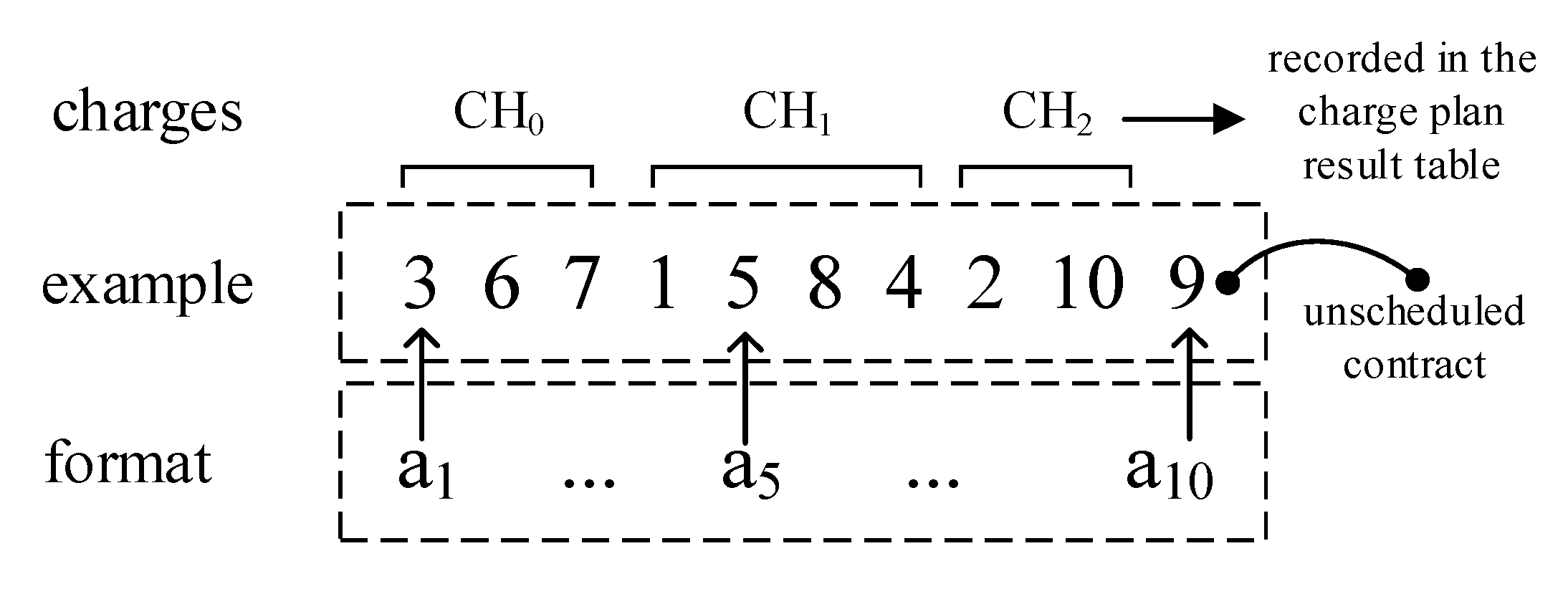
3.1. Chromosome Encoding
3.2. Chromosome Decoding
- Step (1)
- Start a cycle according to chromosome length N.
- Step (2)
- In each cycle, accumulate weight gi of contract ai corresponding to gene position i of the current chromosome.
- Step (3)
- Determine whether the accumulated weight exceeds the furnace capacity. If not, record the contract ai.
- Step (4)
- If yes, subtract weight gi from the accumulated weight and record the accumulated contract as the number of charges in the charge plan result table.
- Step (5)
- Run the next cycle until the algorithm iterates N times.
3.3. Calculation of the Fitness Function
3.4. Genetic Operators
- (1)
- Selection operators
- (2)
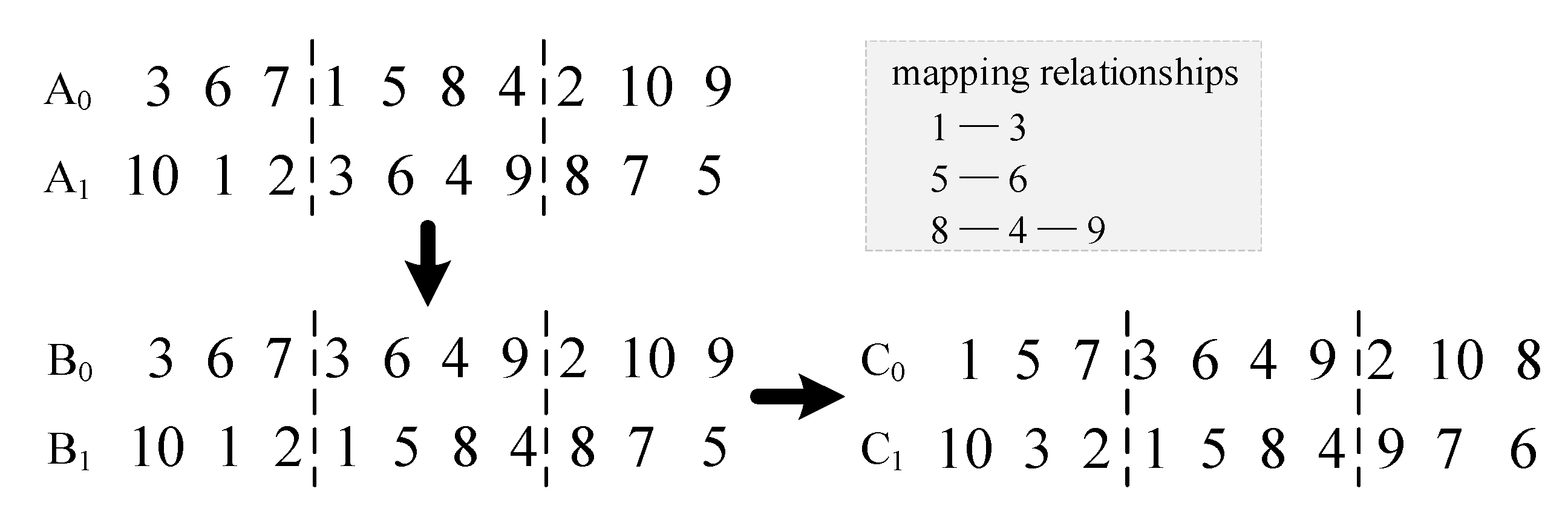
- Crossover operators
- Step (1)
- All chromosomes are paired in the order in which they exist in the population. If the number of chromosomes is odd, the last chromosome is copied directly and does not participate in the crossover operation.
- Step (2)
- The starting and ending positions of the genes to be swapped in a pair of parental chromosomes (A0\A1) are generated randomly.
- Step (3)
- Intermediate chromosomes (B0\B1) are obtained by swapping the genes of two chromosomes and scrambling the sequences, respectively.
- Step (4)
- Conflict detection. The algorithm establishes the mapping relationships between two groups of genes that need to be exchanged in A0\A1. Then, it replaces a conflicting gene in B0\B1 according to the mapping relationship. Finally, a new pair of progeny chromosomes (C0\C1) is formed.
- (3)
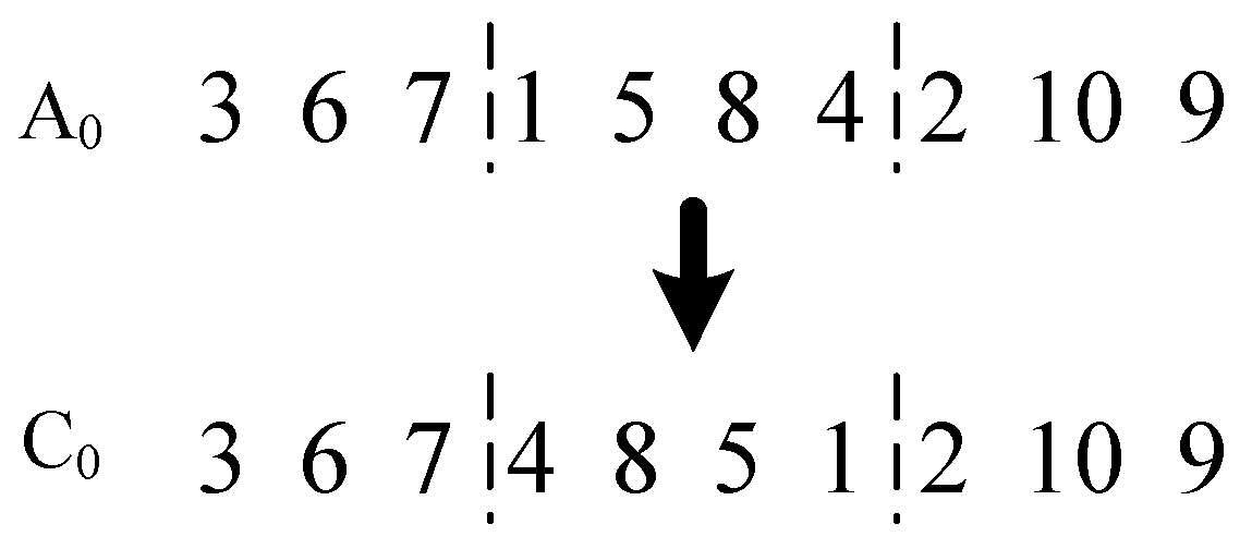
- Mutation operators
4. Application Case and Analysis
4.1. Application Case
4.2. Discussion and Analysis of Results
- (1)
- Proposed model
- (2)
- Proposed algorithm
4.3. Practical Examples
5. Conclusions and Future Prospects
- (1)
- The results of model analysis confirmed the correctness of the developed charge plan model. We found that the optimal objective function value was 123.10, the total amount of the residual material was 294 t, and the solving time was 587.10 s.
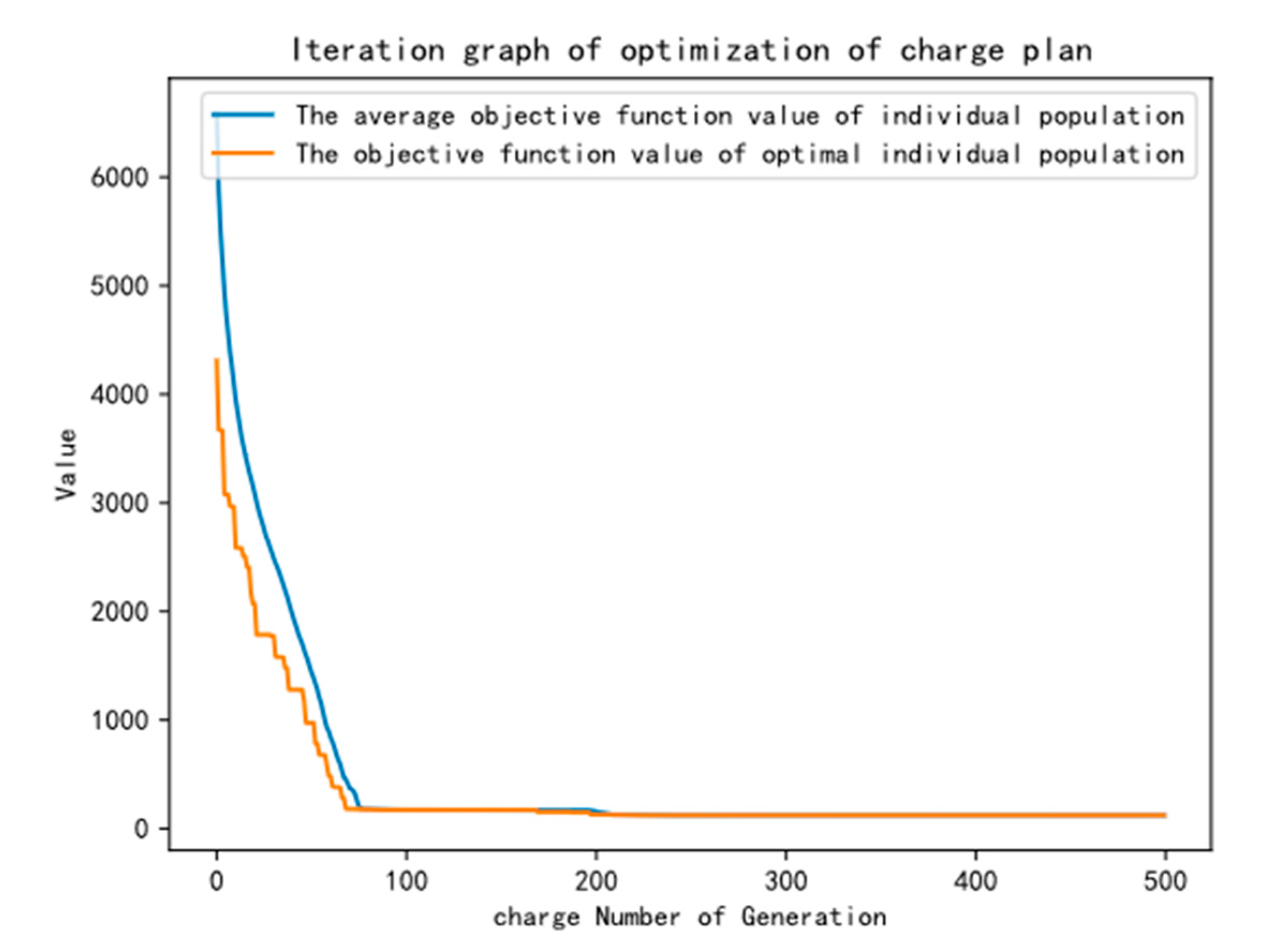
- (2)
- Through algorithm analysis, we demonstrated that IEGA is more effective than EGA and SGA. In the process of solving the model, each iteration of IEGA requires two selection operations, one crossover operation and one mutation operation, which improves the speed of searching for the optimal solution of the algorithm and prevents the algorithm from tending to the local optimal solution.
- (3)
- Using the SM-CC production planning system, the processing time in the SM-CC was shortened by about 20 min. The average number of broken casting times was reduced from 0.8 to 0.3, and the residual materials decreased from 11.2 t to 2.3 t.
Author Contributions
Funding
Acknowledgments
Conflicts of Interest
References
- Ouelhadj, D. A Multi-Agent System for the Integrated Dynamic Scheduling of Steel Production. Ph.D. Thesis, The University of Nottingham, Nottingham, UK, 2003. [Google Scholar]
- Yan, L. Research on the construction of optimal charge plan model based on steelmaking. China Met. Bull. 2019, 7, 3–4. [Google Scholar]
- Tang, L.X. Production Batch Planning Theory and Its Application in CIMS; Science Press: Beijing, China, 1999. [Google Scholar]
- Tang, L.X.; Yang, Z.H.; Wang, M.G. Model and algorithm of furnace charge plan for steelmaking—Continuous casting production scheduling. J. Northeast. Univ. 1996, 17, 440–445. [Google Scholar]
- Huang, K.W.; Lu, K.B.; Wang, D.W. Dynamic programming algorithm and optimization model of charge design for steelmaking. J. Northeast. Univ. Nat. Sci. 2006, 27, 138. [Google Scholar]
- Cheng, Y.; Sun, F.Q.; Chen, T.; Liu, S.X. Optimization methods for batch planning of steelmaking-continuous casting production with two-wide-streams. In Proceedings of the Chinese Automation Congress, Xi’an, China, 30 November–2 December 2018. [Google Scholar]
- Ma, T.M.; Luo, X.C.; Chai, T.Y. Hybrid optimization for charge planning considering the leftover of charge and width. J. Syst. Eng. 2013, 28, 694–701. [Google Scholar]
- Ouelhadj, D.; Cowling, P.I.; Petrovic, S. Utility and stability measures for agent-based dynamic scheduling of steel continuous casting. In Proceedings of the IEEE International Conference on Robotics & Automation, Taipei, China, 14–19 September 2003. [Google Scholar]
- Wang, H.B.; Xu, A.J.; Yao, L.; Tian, N.Y. Modeling of steelmaking—Continuous casting manufacturing flow using colored Petri nets and solution of optimized scheduling. J. Univ. Sci. Technol. Beijing 2010, 32, 938–945. [Google Scholar]
- Feng, Z.J.; Yang, G.K.; Du, B.; Huang, K.W. Two stage optimization algorithms based on heuristic and linear programming in continuous casting scheduling. Metall. Ind. Autom. 2005, 29, 18–22. [Google Scholar]
- Mao, K.; Pan, Q.K.; Pang, X.F.; Chai, T.Y. A novel lagrangian relaxation approach for a hybrid flow shop scheduling problem in the steelmaking-continuous casting process. Eur. J. Oper. Res. 2014, 236, 51–60. [Google Scholar] [CrossRef]
- Lu, Y.M.; Tian, N.Y.; Xu, A.J.; He, D.F. Batch planning and scheduling of steelmaking-continuous casting based on integrated production. Inf. Control. 2011, 40, 715–720. [Google Scholar]
- Tang, L.X.; Guan, J.; Hu, G.F. Steelmaking and refining coordinated scheduling problem with waiting time and transportation consideration. Comput. Ind. Eng. 2010, 58, 239–248. [Google Scholar] [CrossRef]
- Yuan, S.P.; Li, T.K.; Wang, B.L. Improved fast elitist non-dominated sorting genetic algorithm for multi-objective steelmaking-continuous casting production scheduling. Comput. Integr. Manuf. Syst. 2019, 25, 115–124. [Google Scholar]
- Gong, Y.M.; Zheng, Z.; Jian, J.Y.; Gao, X.Q. Multi-objective optimization for charge-choosing and casting start time decision-making on continuous casters. Comput. Integr. Manuf. Syst. 2017, 23, 261–272. [Google Scholar]
- Chen, B. Optimal furnace steelmaking plans based on immune genetic algorithm. J. Southwest China Norm. Univ. 2018, 9, 30–37. [Google Scholar]
- Liu, Q.; Wang, B.; Yang, J.P.; Zhang, J.S.; Gao, S.; Guan, M.; Li, T.-K.; Gao, W.; Liu, Q. Progress of research on steelmaking—Continuous casting production scheduling. Chin. J. Eng. 2020, 2, 144–153. [Google Scholar]
- Lei, Y.J.; Zhang, S.W.; Li, X.W.; Zhou, C.M. MATLAB Genetic Algorithm Toolbox and Its Application; Xidian University Press: Xi’an, China, 2005. [Google Scholar]
- Blickle, T.; Thiele, L. A comparison of selection schemes used in evolutionary algorithms. Evol. Comput. 1995, 4, 361–394. [Google Scholar] [CrossRef]
- Larrañaga, P.; Kuijpers, C.M.H.; Murga, R.H.; Inza, I.; Dizdarevic, S. Genetic algorithms for the travelling salesman problem: A review of representations and operators. Artif. Intell. Rev. 1999, 13, 129–170. [Google Scholar] [CrossRef]
- Suh, J.Y.; Gucht, D.V. Incorporating heuristic information into genetic search. In Genetic Algorithms and Their Applications, Proceedings of the Second International Conference on Genetic Algorithms; The Massachusetts Institute of Technology: Cambridge, MA, USA; L. Erlhaum Associates: Hillsdale, NJ, USA, 1987. [Google Scholar]
- Lv, J. Application in parameter estimation of nonlinear system based upon improved genetic algorithms of cataclysmic mutation. J. Chongqing Norm. Univ. 2004, 21, 13–16. [Google Scholar]
- Ma, J.S.; Liu, G.Z.; Jia, Y.L. The big mutation: An operation to improve the performance of genetic algorithms. Control Theory Appl. 1998, 15, 404–408. [Google Scholar]
- Majumdar, J.; Bhunia, A.K. Elitist-genetic-algorithm-approach-for-Assignment-Problem. AMO 2006, 8, 135–149. [Google Scholar]
- Cormen, T.H.; Leiserson, C.E.; Rivest, R.L.; Stein, C. Introduction to Algorithms; The MIT Press: Cambridge, UK, 2009. [Google Scholar]

| Symbol | Definition |
|---|---|
| Xik/Xjk | =1. Charge k includes contract i/j. |
| =0. Charge k does not include contract i/j. | |
| Yk | Residual material quantity of charge k. |
| L | Total number of charges to be planned. |
| N | Total number of contracts. |
| W | Furnace capacity. |
| gi | Weight of contract i. |
| PR | Penalty cost of residual material. |
| PiU | Penalty cost of the contract i not selected. |
| Pijc/Pijw/Pijd | When contracts i and j form a charge, the penalty cost caused by the difference in steel grade, width, and delivery time. |
| Pc/Pw/Pd | Penalty cost coefficient caused by the difference in steel grade, width, and delivery time when contracts i and j form a charge. |
| ci/wi/di | Steel grade, width, and delivery time of contract i. |
| Rc | Maximum difference in steel grade in the same charge. |
| Rw | Maximum width adjustment range of the contract in the same charge. |
| Rd | Maximum delivery time interval between contracts in the same charge. |
| α1/α2/α3 | Weight coefficients of the three objective functions whose sum is 1, which are equal to 1/3 in this article. |
| Contract No. | Official Number | Steel Grade Code | Steel Grade | Width/mm | Delivery Time/d | Weight/t | Cancellation Penalty |
|---|---|---|---|---|---|---|---|
| 1 | 6179921 | BQ37701F | 24 | 1495 | 30 | 70 | 10 |
| 2 | 6179928 | BQ69200F | 24 | 1533 | 30 | 63 | 10 |
| 3 | 6172135 | BN37704F | 21 | 1525 | 30 | 75 | 10 |
| 4 | 6172233 | CG61100F | 23 | 1505 | 30 | 75 | 10 |
| 5 | 6156607 | CB61200F | 24 | 1474 | 30 | 72 | 10 |
| 6 | 6172129 | BQ37704F | 24 | 1474 | 30 | 65 | 10 |
| 7 | 6172242 | BN47701F | 22 | 1474 | 30 | 75 | 10 |
| 8 | 6180591 | BQ38701F | 23 | 1472 | 30 | 91 | 10 |
| 9 | 6172242 | CB61200F | 22 | 1472 | 30 | 75 | 10 |
| 10 | 6180591 | AC06300R | 11 | 1494 | 30 | 91 | 10 |
| 11 | 6180572 | AC06300R | 12 | 1488 | 30 | 81 | 10 |
| 12 | 6180570 | AC06300F | 11 | 1476 | 30 | 73 | 10 |
| 13 | 6180352 | AC06300R | 11 | 1474 | 30 | 91 | 10 |
| 14 | 6179558 | AC06300R | 12 | 1476 | 30 | 74 | 10 |
| 15 | 6180330 | AC06300R | 11 | 1472 | 30 | 61 | 10 |
| 16 | 6180615 | AC06300R | 11 | 1472 | 30 | 61 | 10 |
| 17 | 6180619 | AC06300F | 12 | 1472 | 30 | 61 | 10 |
| 18 | 6180009 | AC06300R | 11 | 1471 | 30 | 74 | 10 |
| 19 | 6180193 | AC06300R | 11 | 1471 | 30 | 72 | 10 |
| 20 | 6176823 | AC06300R | 12 | 1470 | 30 | 74 | 10 |
| 21 | 6177181 | AC06300R | 12 | 1470 | 30 | 72 | 10 |
| 22 | 6177184 | AC06300F | 10 | 1464 | 30 | 76 | 10 |
| 23 | 6180189 | AC13500R | 11 | 1464 | 30 | 62 | 10 |
| 24 | 6176670 | AC13500R | 10 | 1258 | 15 | 74 | 10 |
| 25 | 6178762 | AC13500R | 10 | 1255 | 15 | 64 | 10 |
| 26 | 6180571 | AC06900F | 10 | 1243 | 30 | 81 | 10 |
| 27 | 6180578 | AC10400F | 10 | 1243 | 30 | 61 | 10 |
| 28 | 6179559 | BC06800F | 12 | 1241 | 15 | 85 | 10 |
| 29 | 6179987 | BC06800F | 11 | 1241 | 15 | 65 | 10 |
| 30 | 6180618 | AC05400F | 11 | 1241 | 30 | 81 | 10 |
| 31 | 6122828 | AK43701F | 23 | 1569 | 30 | 66 | 10 |
| 32 | 6180060 | BQ37704F | 24 | 1525 | 30 | 73 | 10 |
| 33 | 6179923 | BQ69200F | 24 | 1524 | 30 | 65 | 10 |
| 34 | 6169455 | BH02900F | 15 | 1471 | 20 | 74 | 10 |
| 35 | 6174345 | BC06900F | 12 | 1270 | 15 | 87 | 100 |
| 36 | 6154910 | AC06300R | 12 | 1270 | 15 | 93 | 100 |
| 37 | 6179629 | AC06300R | 12 | 1269 | 15 | 93 | 100 |
| 38 | 6179877 | AC06300F | 12 | 1269 | 15 | 93 | 100 |
| 39 | 6178809 | AC06300F | 12 | 1268 | 15 | 87 | 100 |
| 40 | 6178952 | AC06300R | 10 | 1268 | 15 | 77 | 100 |
| Times | Residual Materials | OOFV of the Charge Plan | Solving Time/s |
|---|---|---|---|
| 1 | 294 | 123.18 | 635.68 |
| 2 | 294 | 123.10 | 587.10 |
| 3 | 362 | 144.98 | 637.23 |
| 4 | 313 | 128.62 | 559.05 |
| 5 | 360 | 146.64 | 610.30 |
| 6 | 294 | 123.10 | 649.24 |
| 7 | 572 | 306.28 | 552.84 |
| 8 | 445 | 171.46 | 571.05 |
| 9 | 369 | 148.44 | 660.87 |
| 10 | 275 | 125.76 | 663.73 |
| mean | 357.8 | 154.16 | 612.71 |
| Charge No. | Contract No. | Official Number | Steel Grade Code | Steel Grade | Width/mm | Delivery Time/d | Weight/t | Residual Material/t |
|---|---|---|---|---|---|---|---|---|
| 1 | 4 | 6172233 | CG61100F | 23 | 1505 | 30 | 75 | 18 |
| 1 | 6179921 | BQ37701F | 24 | 1495 | 30 | 70 | ||
| 6 | 6172129 | BQ37704F | 24 | 1474 | 30 | 65 | ||
| 5 | 6156607 | CB61200F | 24 | 1474 | 30 | 72 | ||
| 2 | 28 | 6179559 | BC06800F | 12 | 1241 | 15 | 85 | 35 |
| 39 | 6178809 | AC06300F | 12 | 1268 | 15 | 87 | ||
| 37 | 6179629 | AC06300R | 12 | 1269 | 15 | 93 | ||
| 3 | 26 | 6180571 | AC06900F | 10 | 1243 | 30 | 81 | 77 |
| 27 | 6180578 | AC10400F | 10 | 1243 | 30 | 61 | ||
| 30 | 6180618 | AC05400F | 11 | 1241 | 30 | 81 | ||
| 4 | 8 | 6180591 | BQ38701F | 23 | 1472 | 30 | 91 | 59 |
| 9 | 6172242 | CB61200F | 22 | 1472 | 30 | 75 | ||
| 7 | 6172242 | BN47701F | 22 | 1474 | 30 | 75 | ||
| 5 | 29 | 6179987 | BC06800F | 11 | 1241 | 15 | 65 | 20 |
| 25 | 6178762 | AC13500R | 10 | 1255 | 15 | 64 | ||
| 24 | 6176670 | AC13500R | 10 | 1258 | 15 | 74 | ||
| 40 | 6178952 | AC06300R | 10 | 1268 | 15 | 77 | ||
| 6 | 2 | 6179928 | BQ69200F | 24 | 1533 | 30 | 63 | 33 |
| 32 | 6180060 | BQ37704F | 24 | 1525 | 30 | 73 | ||
| 33 | 6179923 | BQ69200F | 24 | 1524 | 30 | 65 | ||
| 31 | 6122828 | AK43701F | 23 | 1569 | 30 | 66 | ||
| 7 | 38 | 6179877 | AC06300F | 12 | 1269 | 15 | 93 | 27 |
| 35 | 6174345 | BC06900F | 12 | 1270 | 15 | 87 | ||
| 36 | 6154910 | AC06300R | 12 | 1270 | 15 | 93 | ||
| 8 | 11 | 6180572 | AC06300R | 12 | 1488 | 30 | 81 | 10 |
| 14 | 6179558 | AC06300R | 12 | 1476 | 30 | 74 | ||
| 20 | 6176823 | AC06300R | 12 | 1470 | 30 | 74 | ||
| 17 | 6180619 | AC06300F | 12 | 1472 | 30 | 61 | ||
| 9 | 13 | 6180352 | AC06300R | 11 | 1474 | 30 | 91 | 1 |
| 23 | 6180189 | AC13500R | 11 | 1464 | 30 | 62 | ||
| 19 | 6180193 | AC06300R | 11 | 1471 | 30 | 72 | ||
| 18 | 6180009 | AC06300R | 11 | 1471 | 30 | 74 | ||
| 10 | 12 | 6180570 | AC06300F | 11 | 1476 | 30 | 73 | 14 |
| 15 | 6180330 | AC06300R | 11 | 1472 | 30 | 61 | ||
| 16 | 6180615 | AC06300R | 11 | 1472 | 30 | 61 | ||
| 10 | 6180591 | AC06300R | 11 | 1494 | 30 | 91 |
| Methods | Population Size | Iterations | Vo1 | To2 | Mo3 | Vc4 | Tc5 | Mc6 |
|---|---|---|---|---|---|---|---|---|
| IEGA | 1000 | 500 | 123.10 | 587.10 | 294 | 138.03 | 615.06 | 336.8 |
| EGA | 1000 | 1000 | 123.10 | 754.84 | 294 | 162.54 | 1095.56 | 348.5 |
| SGA | 2000 | 1000 | 2279.2 | 2163.27 | 447 | 2377.88 | 4173.17 | 511.20 |
| Contrast Items | Processing Time of SM-CC/min | The Number of Times the Broken Casting | Residual Materials/t |
|---|---|---|---|
| System application | 183.5 | 0.3 | 2.3 |
| No system application | 206.4 | 0.8 | 11.2 |
© 2020 by the authors. Licensee MDPI, Basel, Switzerland. This article is an open access article distributed under the terms and conditions of the Creative Commons Attribution (CC BY) license (http://creativecommons.org/licenses/by/4.0/).
Share and Cite
Yuan, F.; Wu, S.; Song, W.; Xu, A. Charge Plan Model for Steelmaking-Continuous Casting Section. Metals 2020, 10, 1196. https://doi.org/10.3390/met10091196
Yuan F, Wu S, Song W, Xu A. Charge Plan Model for Steelmaking-Continuous Casting Section. Metals. 2020; 10(9):1196. https://doi.org/10.3390/met10091196
Chicago/Turabian StyleYuan, Fei, Shuangping Wu, Wei Song, and Anjun Xu. 2020. "Charge Plan Model for Steelmaking-Continuous Casting Section" Metals 10, no. 9: 1196. https://doi.org/10.3390/met10091196
APA StyleYuan, F., Wu, S., Song, W., & Xu, A. (2020). Charge Plan Model for Steelmaking-Continuous Casting Section. Metals, 10(9), 1196. https://doi.org/10.3390/met10091196