DFT-CEF Approach for the Thermodynamic Properties and Volume of Stable and Metastable Al–Ni Compounds

Abstract

The Al–Ni system has been intensively studied both experimentally and theoretically. Previous first-principles calculations based on density-functional theory (DFT) typically investigate the stable phases of this system in their experimental stoichiometry. In this work, we present DFT calculations for the Al–Ni system that cover stable and metastable phases across the whole composition range for each phase. The considered metastable phases are relevant for applications as they are observed in engineering alloys based on Al–Ni. To model the Gibbs energies of solid phases of the Al–Ni system, we combine our DFT calculations with the compound energy formalism (CEF) that takes the Bragg–Williams–Gorsky approximation for the configurational entropy. Our results indicate that the majority of the investigated configurations have negative energy of formation with respect to Al fcc and Ni fcc. The calculated molar volumes for all investigated phases show negative deviations from Zen’s law. The thermodynamic properties at finite temperatures of individual phases allow one to predict the configurational contributions to the Gibbs energy. By applying a fully predictive approach without excess parameters, an acceptable topology of the DFT-based equilibrium phase diagram is obtained at low and intermediate temperatures. Further contributions can be added to improve the predictability of the method, such as phonons or going beyond the Bragg–Williams–Gorsky approximation that overestimates the stability range of the ordered phases. This is clearly demonstrated in the fcc order/disorder predicted metastable phase diagram.

1. Introduction

The compound energy formalism (CEF) [1] is a well established framework used to model Gibbs energies as a function of temperature, composition and pressure. The knowledge of the Gibbs energies allows for the calculation of thermodynamic properties and equilibrium between phases. This procedure is used in the so called Calphad method [2] to obtain calculated phase diagrams. Quantum-mechanical approaches such as density functional theory (DFT) [3] can make significant contributions to Calphad, e.g., with regard to the development of multicomponent databases based on information on stable and metastable binary phases, particularly after recent improvements on the models for multicomponent and structurally complex phases, such as the $\sigma$ phase [4]. In this study we used DFT to scan the configuration space in the whole composition range for each phase in its stable or metastable state. The Al–Ni system was selected due to its significant technological and theoretical importance. It is a prototype system for order–disorder transformations and the base system of Ni-based superalloys that are used in turbine blades for aviation and power generation [5,6]. The design of these alloys requires knowledge of potential metastable phases [7,8] that can deteriorate the mechanical properties. In contrast to a recent publication [9] on the Al–Ni system where DFT calculations were carried out for fcc and bcc ordering families, we include ordered fcc, bcc and hcp phases, along with D0${}_{11}$, D5${}_{13}$ and the topologically close-packed (TCP) phases $\sigma$, $\mu$, $\chi$, A15, C14, C15 and C36. We followed the methodology previously used for Re-X (X = Ta, V, W) systems studying topologically closed-packed (TCP) phases [10]. In this way, finite temperature phase stability was investigated using the Bragg–Williams–Gorsky approximation (BWG) as implemented in the Thermo-Calc software [11,12] for the description of the configurational entropy. The methodology used in this work is referred to as the DFT-CEF approach and differs from other published studies which also used DFT calculations as input data, these differences are briefly described in

Table 1. Different thermodynamic approaches in the literature.

Reference	Entropy Model	TDB Available	Approach
This work	BWG	yes	DFT-CEF + no excess parameters reference state at 0 K
Al–Ni [9]	CE/MC	no	DFT 0 K
ATAT [13]	CE/CVM/MD	yes	DFT + finite temperature
Co-Ta [14]	BWG + excess	yes	DFT-CEF + excess parameters reference state at 298.15 K (SGTE)

.

The structure of the paper is as follows: details of the methodology are indicated in Section 2. In Section 3.1 and Section 3.2 we discuss the structural stability of the elements and the binary phases at 0 K and the trends of molar volumes with composition. The thermodynamic properties of the individual phases at finite temperatures are given in Section 3.3. The phase stability as a function of temperature and composition is presented in the phase diagram in Section 3.4. At the end of this section, the overcoming of a major drawback of the thermodynamic model is discussed, and finally, we conclude in Section 4.

2. Methodology

2.1. DFT Calculations

Electronic-structure calculations based on DFT were performed using the Vienna Ab initio Simulation Package (VASP) [15,16,17] within a high-throughput environment [18]. We used projector augmented wave (PAW) pseudopotentials and the generalized gradient approximation (GGA) of Perdew et al. [19] for the exchange-correlation functional. A cut-off energy of 400 eV and Monkhorst-Pack [20] k-point meshes with a density of 0.020 Å${}^3$ were sufficient to converge differences in the formation energy to less than 1 meV/atom. Spin-polarization was used for the calculations and full relaxation (P ≈ 0 GPa) of all the structures was performed. Initial magnetic moments were set to zero, as a comprehensive study of the effects of magnetism with exhaustive sampling of magnetic configurations for all considered phases would have required a large number of DFT calculations and a corresponding treatment in the Calphad formalism that was beyond the scope of this work.

The formation energies of the compound phases were obtained from the total energy of a given binary configuration, $\varphi$, of crystal structure, $\Gamma$ and composition ($x_{\mathrm{Al}}$, $x_{\mathrm{Ni}}$) with respect to the energy of the pure elements in the ground-state structure fcc of Al and Ni:

$$E_f^{\Gamma ,\varphi }=E_0^{\Gamma ,\varphi }-\left(\frac{x_{\mathrm{Al}}}{x_{\mathrm{Al}}+x_{\mathrm{Ni}}}\right)E_0^{\mathrm{fcc},\mathrm{Al}}-\left(\frac{x_{\mathrm{Ni}}}{x_{\mathrm{Al}}+x_{\mathrm{Ni}}}\right)E_0^{\mathrm{fcc},\mathrm{Ni}}$$

(1)

where $E_f^{\Gamma ,\varphi }$ is the formation energy of the binary configuration; and $E_0^{\Gamma ,\varphi }$, $E_0^{\mathrm{fcc},\mathrm{Al}}$ and $E_0^{\mathrm{fcc},\mathrm{Ni}}$ are the total energies per atom for the binary configuration, fcc Al and fcc Ni, respectively. The energy-volume results were fitted using the Murnaghan equation of state. At 0 K and 0 Pa, $E_f^{\Gamma ,\varphi }$ corresponds to the enthalpy of formation of the configuration $\varphi$ in the structure $\Gamma$.

2.2. Thermodynamic Modeling

The general expression of the Gibbs energy for a solid phase at T≠ 0 K is

$$G=U+PV-TS$$

(2)

where the pressure-volume term, PV, vanishes for our fully relaxed structures. If the entropy term includes only the configurational contribution (no vibrational entropy), an equivalent formulation of the CEF has the following expression.

$$G=E^{\mathrm{srf}}-T{S}^{\mathrm{conf}}$$

(3)

where $E^{\mathrm{srf}}$ is the surface of reference, the sum of total energies of all the configurations, and $S^{\mathrm{conf}}$ is the configurational entropy. In this work the configurational contribution is restricted to the BWG approximation [1,21] and no interaction parameters were considered to obtain temperature-dependent properties (see Section 3.4). All considered phases were modeled using Equation (3) and the energies of each individual configuration were calculated using DFT, as indicated in the previous section. The number of possible configurations for each phase was determined by the permutations of Al and Ni on the respective Wyckoff positions (see Tables 3 and 4 with A = Ni and B = Al).

The CEF [1,4,22,23] describes the Gibbs energy of a given phase as a function of sublattices (SLs) in its crystal structure. The number of considered SLs will determine the number of configurations or end-members (limiting compositions) needed to describe the phase. For bcc, fcc and hcp solution phases a four-sublattice (4SL) model was used. For the TCP phases, for D5${}_{13}$-Al${}_3$Ni${}_2$ and for D0${}_{11}$-Al${}_3$Ni a complete SL description was used; i.e., the Wyckoff sites of each phase determine the total number of SLs and their multiplicity, and the number of sites in each SL. Hence, the $\mu$, $\sigma$ and C36 phases with five Wyckoff positions were modeled with five sublattices. Permuting Al and Ni on the five SLs gave rise to 2${}^5$ = 32 configurations. For a generic phase, $\phi$, with five Wyckoff positions the first and second terms in Equation (3) are defined as

$$\begin{array}{cc}\hfill & E^{\mathrm{srf}}=\sum _{\mathrm{ABCDE}}{y}_{\mathrm{A}}^{\left(1\right)}{y}_{\mathrm{B}}^{\left(2\right)}{y}_{\mathrm{C}}^{\left(3\right)}{y}_{\mathrm{D}}^{\left(4\right)}{y}_{\mathrm{E}}^{\left(5\right)}{E}_f^{\phi ,ABCDE}\hfill \\ \hfill & S^{\mathrm{conf}}=-R\sum _s{a}^s\sum _i{y}_i^{s}ln\left(y_i^s\right)\hfill \end{array}$$

(4)

where $E_f^{\phi ,ABCDE}$ is the structural energy of the end-member ABCDE calculated as explained in Section 2.1, and the summation over all end-members represents the energy of the surface of reference. The second term is the configurational entropy with $a^s$ being the number of sites in sublattice $\mathit{s}$, $y_i^s$ the site fraction of component $\mathit{i}$ in sublattice $\mathit{s}$ and $\mathit{R}$ the gas constant.

The structural energy of the configuration with the same element in all SLs, i.e., $E_f^{\phi ,AAAAA}$ in Equation (4) represents the difference between a given crystal structure and the reference structure of element A. In this work we take the ground-state structure fcc-A1 of Al and Ni as reference states at 0 K. This structural energy difference is an essential parameter to define the Gibbs energies of competing phases and is referred to as lattice stability.

In this work we investigated the lattice stabilities of Al–Ni in eleven crystal structures with respect to the energy of the fcc-A1 ground-state structure at 0 K. The formation energies of all possible configurations generated by permutation of Al and Ni in the different Wyckoff positions were calculated for: nearly all TCP phases, for the D5${}_{13}$-Al${}_3$Ni${}_2$ and D0${}_{11}$-Al${}_3$Ni phases stable in this system and for several ordered fcc, bcc and hcp phases (see Section 3.2). The liquid phase and the Al${}_3$Ni${}_5$ phase were not investigated in the present work.

The thermodynamic calculations were done using the Thermo-Calc Gibbs energy minimizer software version 2020a [11,12] and a Gibbs energy set assembled with the DFT results. The TDB file is provided in the Supplementary Materials.

3. Results

3.1. Structural Stability at 0 K for Al And Ni

The DFT-calculated structural energies or lattice stabilities along with relaxed molar volumes V${}_0$ and bulk moduli B${}_0$ for pure Al and Ni at 0 K are presented in

Table 2. DFT calculated lattice stabilities, ΔH, with respect to fcc-A1 ($E_0^{\Gamma ,\mathrm{i}}-$$E_0^{\mathrm{fcc},\mathrm{i}}$; cf. Equation (1)), relaxed volumes V${}_0$ and bulk moduli B${}_0$ of different Al and Ni structures compared with values available in the literature.

Aluminium
Ref.	A1	A2	A3	A15	A12($\mathbf{\chi }$)	D8${}_b$($\mathbf{\sigma }$)	$\mathbf{\mu }$	C36	C14	C15	D5${}_{13}$	D0${}_{11}$
$\Delta$H (kJ/mol)
This work	0.0	9.3	3.2	7.7	5.1	6.3	10.0	15.0	14.3	15.6	17.1	1.4
PAW-PW91 [24]	0.0	9.7	-	7.5	4.9	6.5	9.7	-	13.9	15.1	-	-
PAW-PW91 [25]	0.0	9.21	2.85	-	-	-	-	-	-	-	-	-
SGTE [26] ${}^a$	0.0	10.1	5.5	-	-	-	-	-	-	-	-	-
V${}_0$ (Å${}^3$/at)
This work	16.48	16.91	16.64	16.93	17.13	16.91	17.31	17.45	17.45	17.43	18.78	16.59
PAW-PBE [27]	16.71	-	-	-	-	-	-	-	-	-	-	-
FPLMTO-GGA [28]	16.63	-	-	-	-	-	-	-	-	-	-	-
LMTO-LDA [29]	15.93	16.17	-	-	-	-	-	-	-	-	-	-
Calphad [30] ${}^a$	-	17.13	16.85	-	-	-	-	-	-	-	-	-
Calphad [31] ${}^a$	16.30	15.50	15.50	-	-	-	-	-	-	-	-	-
B${}_0$ (GPa)
This work	77.6	69.8	73.3	64.7	69.4	74.0	70.1	65.7	66.3	66.5	67.4	76.0
PAW-PBE [27]	72.5	-	-	-	-	-	-	-	-	-	-	-
FPLMTO-GGA [28]	74.4	-	-	-	-	-	-	-	-	-	-	-
LMTO-LDA [29]	87.0	88.0	-	-	-	-	-	-	-	-	-	-
Exp. [32]	72.7	-	-	-	-	-	-	-	-	-	-	-
Nickel
Ref.	A1	A2	A3	A15	A12($\mathbf{\chi }$)	D8${}_b$($\mathbf{\sigma }$)	$\mathbf{\mu }$	C36	C14	C15	D5${}_{13}$	D0${}_{11}$
$\Delta$H (kJ/mol)
This work	0.0	5.3	2.7	11.2	8.3	8.4	14.1	17.5	17.0	18.2	30.5	5.8
PAW-GGA [24]	0.0	8.8	-	12.7	9.1	16.5	16.0	-	19.0	21.3	-	-
PAW-GGA [25]	0.0	9.15	2.13	-	-	-	-	-	-	-	-	-
SGTE [26] ${}^a$	0.0	8.7	2.9	-	-	-	-	-	-	-	-	-
V${}_0$ (Å${}^3$/at)
This work	10.88	10.94	10.92	11.11	11.07	11.08	11.30	11.40	11.39	11.43	12.20	11.08
PAW-PBE [27]	10.90	-	-	-	-	-	-	-	-	-	-	-
PAW-PBE [33]	10.94	-	-	-	-	-	-	-	-	-	-	-
LMTO-LDA [29]	10.53	10.62	-	-	-	-	-	-	-	-	-	-
B${}_0$ (GPa)
This work	199.3	193.7	189.7	185.3	202.1	189.5	177.2	188.5	198.5	183.5	165	145.2
PAW-PBE [27]	190.5	-	-	-	-	-	-	-	-	-	-	-
PAW-PBE [33]	193.0	-	-	-	-	-	-	-	-	-	-	-
LMTO-LDA [29]	248.0	224.0	-	-	-	-	-	-	-	-	-	-

${}^a$ critically assessed experimental data.

and compared with values from the literature.

The first row of Table 2 shows the enthalpy difference between the corresponding structure and the reference structure fcc-A1 of Al and Ni at 0 K. Our results are in good agreement with previous theoretical [24,25,34,35] and experimental [36] works.

On the other hand, rough agreement is found with Scientific Group Thermodata Europe (SGTE) databank values [26]. SGTE is an extensive consistent compilation of lattice stabilities and Gibbs energies based on assessed experimental data widely used in the Calphad framework. Several comparisons between DFT calculation and SGTE have been done in order to combine these methodologies but disagreements were many times evident [37,38]. The conclusions after the works of Wang et al. [25] and Sluiter [24] indicate good agreement for most of the elements with exception of 3d transition metals.

3.2. Phase Stability and Molar Volumes of Binary Phases at 0 K

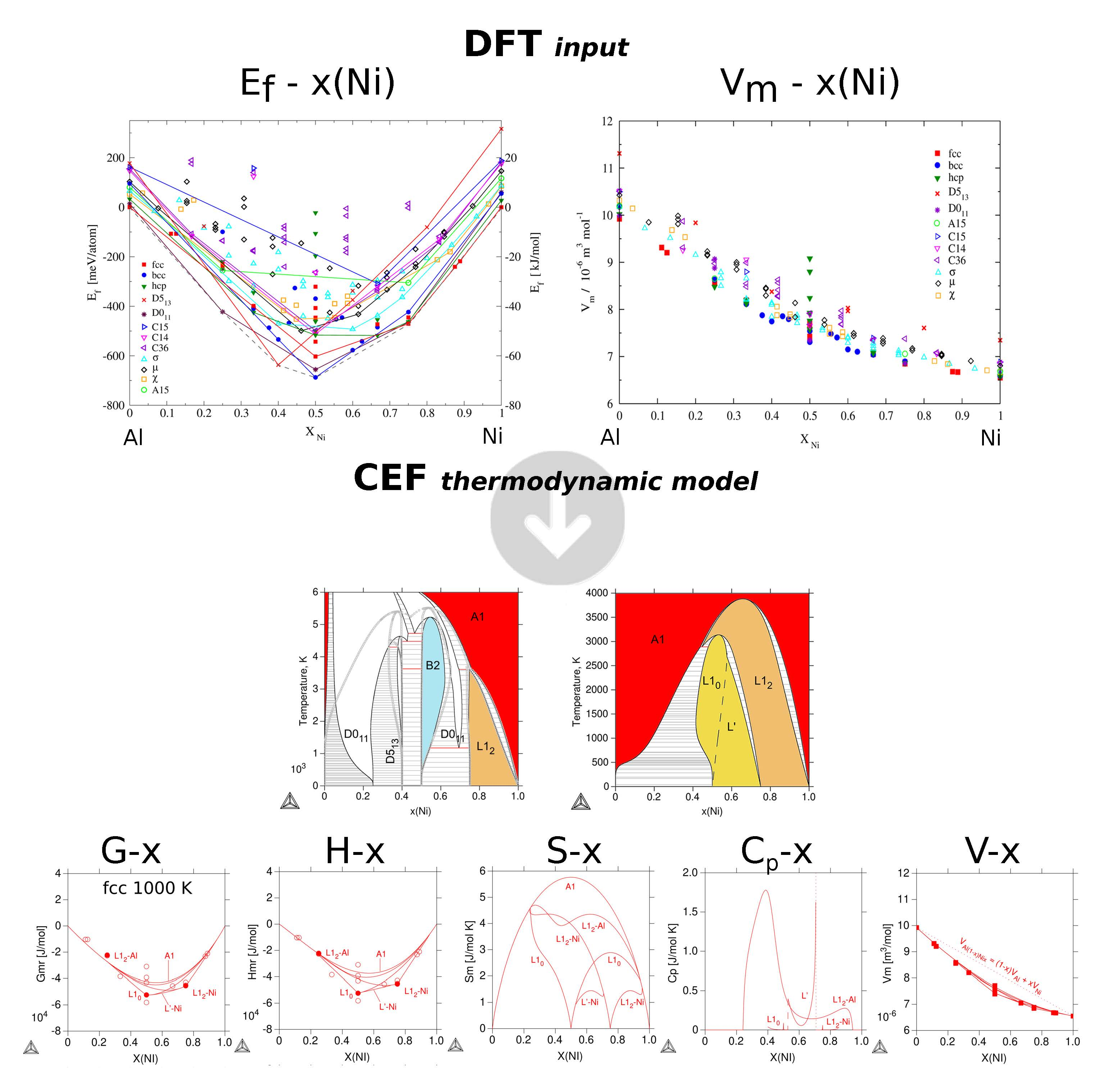
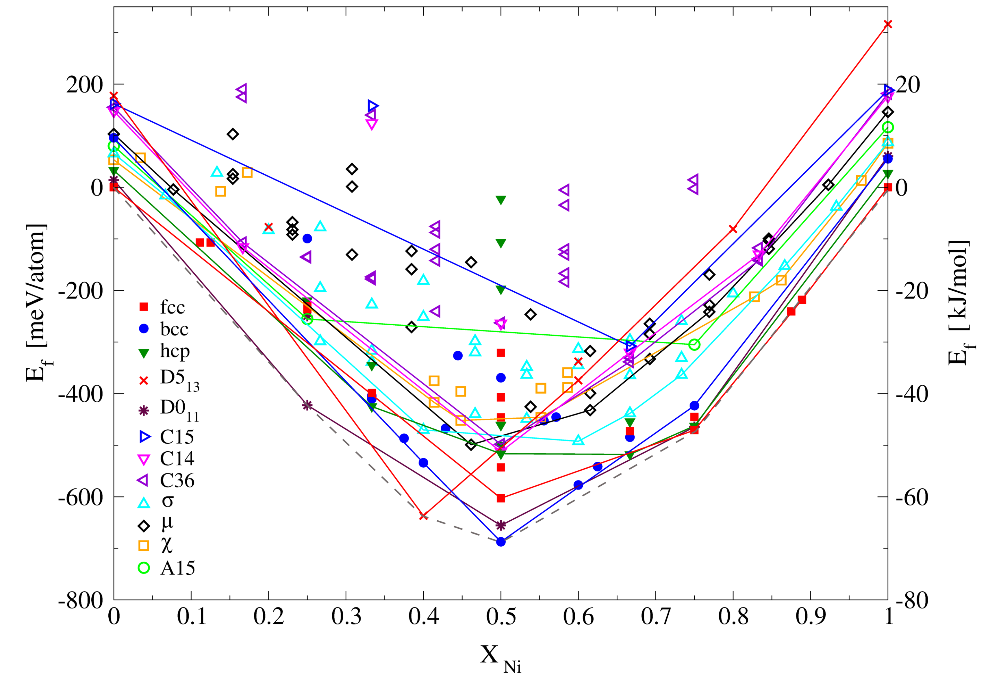
3.2.1. Enthalpies of Formation of Ordered Compounds

The formation enthalpies for stable and metastable ordered compounds of Al–Ni were calculated as indicated in Section 2.1, and the results are presented in Figure 1. The same symbol has been used for configurations in a given crystallographic structure even if the individual structures showed distortions of the unit cell after structural relaxation. The calculated ordered structures for fcc, bcc and hcp are presented

Table 3. Ordered fcc, bcc and hcp phases ofAl–Ni. The atomic composition, Strukturbericht designation (where A = Ni and B = Al), calculated formation energy, Pearson symbol, space group and Wyckoff positions are indicated.

x(Ni)	Strukturbericht	Formation Energy [kJ/mol at]	Pearson Symbol	Space Group	Wyckoff Positions
fcc related
0.0	A1-BB	0.0	cF4 (Cu)	Fmm (225)	4a, 4b, 8c
0.111	Al8Ni-AB8	−10.3	tI18 (NbNi${}_8$)	I4/mmm	2a, 8h, 8i
0.125	D1D7-AB7	−10.3	cF32(Ca${}_7$Ge)	Fmm (225)	4a, 4b, 24d
0.25	D0${}_{22}$-AB3	−22.3	tI8 (Al${}_3$Ti)	I4/mmm (139)	2a, 2b, 4d
0.25	L1${}_2$-AB3	−22.3	cP4 (Cu${}_3$Au)	Pmm (227)	1a, 3c
0.25	D0${}_{23}$-AB3	−22.8	tI16 (Al${}_3$Zr)	I4/mmm (139)	4c, 4d, 4e
0.25	L6${}_0$-AB3	−22.3	tP4 (CuTi${}_3$)	P4/mmm (123)	1a 1c 2e 2e
0.333	$\beta$1$\beta$2-AB2	−38.5	tI6	I4/mmm (139)	-
0.5	CH40-AB	−58.2	tI8(NbP)	I4${}_1$/amd (141)	2a, 2b
0.5	D4-AB	−31.0	-	Fdm	-
0.5	L1${}_0$-AB	−52.4	tP2 (CuAu)	P4/mmm (123)	1a, 1d
0.5	L1${}_1$-AB	−43.0	hR32 (CuPt)	Rm (166)	1a, 1b
0.5	Z2-AB	−39.3	tP8	P4/nmm (129)
0.667	$\beta$1$\beta$2-A2B	−45.6	tI6	I4/mmm (139)
0.75	D0${}_{22}$-A3B	−43.1	tI8 (Al${}_3$Ti)	I4/mmm (139)	2a, 2b, 4d
0.75	L1${}_2$-A3B	−45.4	cP4 (Cu${}_3$Au)	Pmm (227)	1a, 3c
0.75	L6${}_0$-A3B	−45.0	tP4 (CuTi${}_3$)	P4/mmm (123)	1a 1c 2e 2e
0.875	D1D7-A7B	−23.2	cF32(Ca${}_7$Ge)	Fmm (225)	4a, 4b, 24d
0.889	Al8Ni-A8B	−21.1	tI18 (NbNi${}_8$)	I4/mmm	2a, 8h, 8i
1.0	A1-AA	0.0	cF4 (Cu)	Fmm (225)	4a, 4b, 8c
bcc related
0.0	A2-BB	+9.3	cI2 (W)	Imm (229)	2a
0.25	D0${}_3$-AB3	−9.6	cF16 (AlFe${}_3$)	Fmm (225)	4a, 4b, 8c
0.333	C11${}_b$-AB2	−39.6	tl6	I4/mmm (139)	2a, 4e
0.375	PdTi-A3B5	−47.0	-	-	-
0.4	AlOs-A2B3	−51.5	-	-	-
0.428571	B11-A3B4	−45.1	tP4 ($\gamma$CuTi)	P4/nmm (129)	2c
0.444	VZn-A4B5	−31.5	tI18 (V${}_4$Zn5)	I4/mmm (139)	2a, 8h, 8i
0.5	B2-AB	−66.3	cP2 (CsCl)	Pmm (221)	1a, 1b
0.5	B32-AB	−35.6	cF16 (NaTl)	Fdm (227)	8a, 8b
0.555556	VZn-A5B4	−43.7	tI18 (V${}_4$Zn5)	I4/mmm (139)	2a, 8h, 8i
0.571429	B11-A4B3	−43.0	tP4 ($\gamma$CuTi)	P4/nmm (129)	2c
0.6	AlOs-A3B2	−55.7	-	-	-
0.625	PdTi-A5B3	−52.3	-	-	-
0.667	C11${}_b$-A2B	−46.8	tl6	I4/mmm (139)	2a, 4e
0.75	D0${}_3$-A3B	−40.9	cF16 (AlFe${}_3$)	Fmm (225)	4a, 4b, 8c
1.0	A2-AA	+5.3	cI2 (W)	Imm (229)	2a
hcp related
0.0	A3-BB	+3.2	hP2 (Mg)	P6${}_3$/mmc (194)	2c
0.25	D0${}_{19}$-AB3	−21.2	hP8 (Ni${}_3$Sn)	P6${}_3$/mmc (194)	2c, 6h
0.333	B8${}_2$-AB2	−33.3	hP6 (InNi${}_2$)	P6${}_3$/mmc (194)	2a, 2c, 2d
0.333	B${}_b$-AB2	−41.0	hP9 ($\eta$AgZn)	P (147)	1a, 2d, 6g
0.5	hcp-AB	−48.2	hP2	Pm2 (187)	1a, 1f
0.5	B${}_h$-AB	−44.5	hP2 (WC)	Pm2 (187)	1a, 1f
0.5	B${}_h$-BA	−44.5	hP2 (WC)	Pm2 (187)	1a, 1f
0.5	B${}_i$-AB	−19.0	hP8 (AsTi)	P6${}_3$/mmc (194)	2a, 2d, 4f
0.5	B${}_i$-BA	−49.8	hP8 (AsTi)	P6${}_3$/mmc (194)	2a, 2d, 4f
0.5	B8${}_1$-BA	−10.3	hP4 (NiAs)	P6${}_3$/mmc (194)	2a, 2c
0.5	B35-BA	−2.2	hP6 (CoSn)	P6/mmm (191)	1a, 2d, 3f
0.667	B${}_b$-A2B	−43.8	hP9 ($\eta$AgZn)	P (147)	1a, 2d, 6g
0.667	B8${}_2$-A2B	−50.0	hP6 (InNi${}_2$)	P6${}_3$/mmc (194)	2a, 2c, 2d
0.75	D0${}_{19}$-A3B	−44.6	hP8 (Ni${}_3$Sn)	P6${}_3$/mmc (194)	2c, 6h
1.0	A3-AA	+2.7	hP2 (Mg)	P6${}_3$/mmc (194)	2c

.

The convex hull (dashed gray line in Figure 1) indicates the sequence of stable phases at 0 K of Al (A1), Al${}_3$Ni (D0${}_{11}$), Al${}_3$Ni${}_2$ (D5${}_{13}$), AlNi (B2), AlNi${}_3$ (L1${}_2$) and Ni (A1). This sequence of structural stability with chemical composition is in agreement with the experimental correspondence at 298.15 K (except for Al${}_3$Ni${}_5$ that is not considered in this work). Most of the ordered compounds show negative formation energy with respect to Al fcc and Ni fcc.

When metastable and stable phases are energetically close, as in this case, stabilization is viable through phase transformation that can occur with increasing temperature, deformation, external pressure and/or impurities. A critical region was found around 75 at.% Ni where L1${}_2$ is the energetically most favorable compound at 0 K while metastable D0${}_{19}$ (hcp ordering) and L6${}_0$ (fcc ordering) are only ≈ 8 meV/at and ≈ 4 meV/at higher in energy. Starting form the L1${}_2$ structure, the L6${}_0$ corresponds to a slight tetragonal distortion, while the D0${}_{19}$ corresponds to a different sequence of the compact planes. In the Al-rich side, it can be observed that D0${}_{11}$ is the most stable structure at 25 at.% Ni (as expected). However, at 50 and 75 at.%Ni D0${}_{11}$ is close to the respective stable B2 and L1${}_2$ configurations. This proximity in formation energies leads to close energy competition of these compounds at finite temperatures (cf. Section 3.4). The formation energies in Figure 1 are also presented in Table 3 for bcc, fcc and hcp ordered structures, including composition, Strukturbericht (where A = Ni and B = Al), formation energy, Pearson symbol, space group and Wyckoff positions. Shadowed rows indicate the actual orderings used in the 4 SL model; see Section 3.4. In

Table 4. Crystal structures of Al${}_3$Ni${}_2$, Al${}_3$Ni and TCP phases studied in this work. Indicated are the Pearson symbol, space group, Wyckoff positions and number of configurations when allowing Al and Ni in each position.

Phase	Pearson Symbol	Space Group	Wyckoff Positions	Configurations
D5${}_{13}$ (Al${}_3$Ni${}_2$)	hP5 (Al${}_3$Ni${}_2$)	Pm1 (164)	1a 2d 2d	8
D0${}_{11}$ (Al${}_3$Ni)	oP16 (Fe${}_3$C)	Pmna (62)	4c 4c 8d	8
TCP
$\mu$	hR39 (Fe${}_7$W${}_6$)	Rm (166)	3a, 18h, 6c${}_1$, 6c${}_2$, 6c${}_3$	32
D8${}_b$($\sigma$)	tP30 (FeCr)	P4${}_2$/mnm (136)	2a, 4f, 8i${}_1$, 8i${}_2$, 8j	32
A12($\chi$)	cI58 ($\alpha$ Mg)	I3m (217)	2a, 8c, 24g${}_1$, 24g${}_2$	16
A15	cP8 (Cr${}_3$Si)	Pmm (223)	6c, 2a	4
Laves
C14	hP12 (MgZn${}_2$)	P6${}_3$/mmc (194)	2a, 4f, 6h	8
C15	cF24 (MgCu${}_2$)	Fdm (227)	16d, 8a	4
C36	hP24 (MgNi${}_2$)	P6${}_3$/mmc (194)	4e, 4f${}_1$, 4f${}_2$, 6g, 6h	32

the structural details and number of all possible configurations for TCP, D5${}_{13}$ and D0${}_{11}$ phases are presented. For these phases a complete SL description was used with all configurations included in the thermodynamic model, as can be seen in the TDB file and figure provided in the Supplementary Materials.

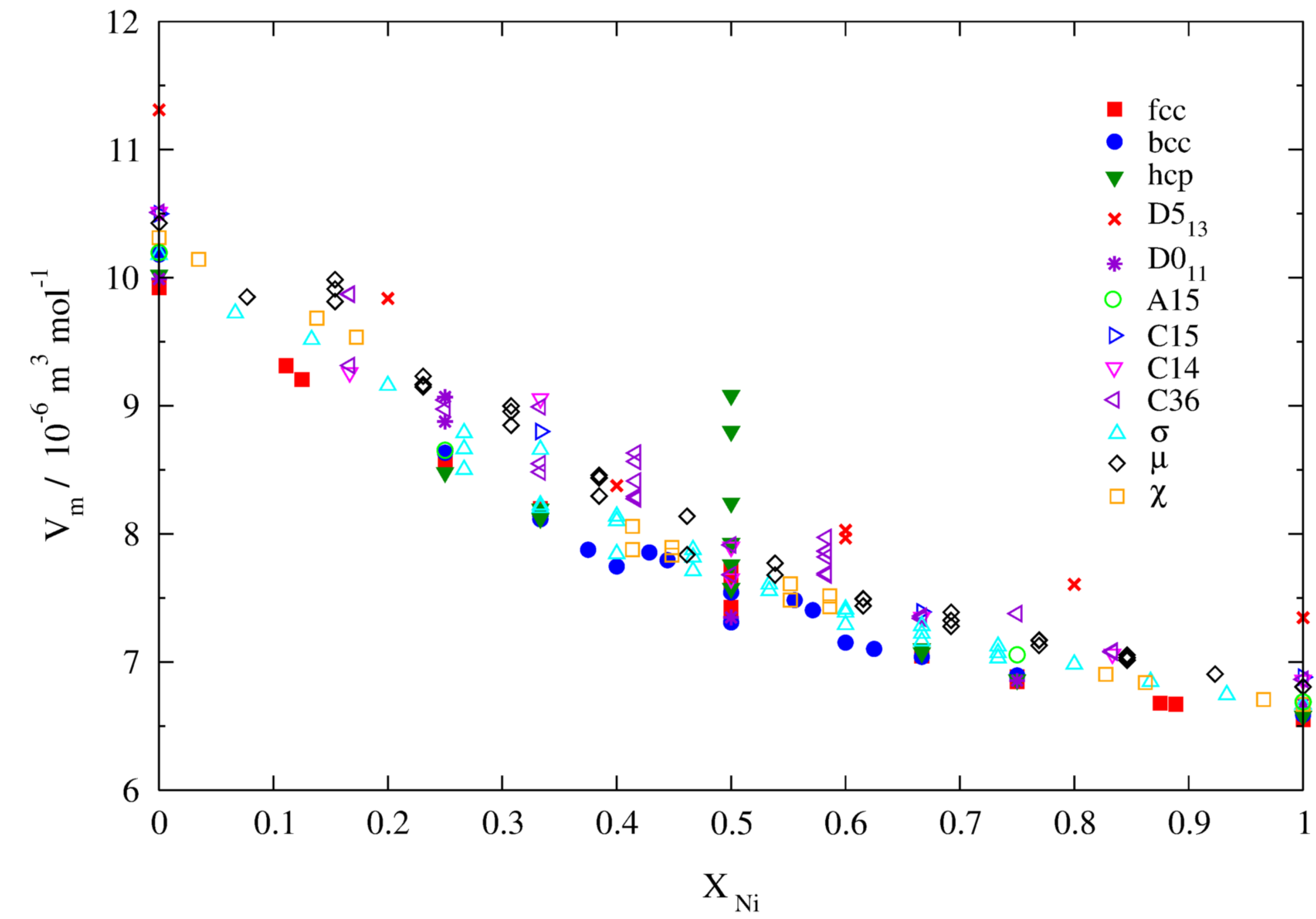
3.2.2. Molar Volumes of Ordered Compounds

In a multiphase equilibria modeling environment such as Calphad, the knowledge of the molar volumes for all the phases is desirable in order to calculate, e.g., volume changes in phase transformations or volume fractions of stable phases. They are of particular importance when coupling thermodynamic descriptions to kinetic models in order to simulate the evolution of microstructures. In the superalloys framework, they are also very important in order to model the mismatch between the ordered and disordered fcc phases that are the basis of the $\gamma$ (A1)/${\gamma }^{\prime }$ (L1${}_2$) microstructure of single-crystal superalloys. The DFT calculated molar volumes of ordered stable and metastable compounds of Al–Ni are presented in Figure 2 as a function of composition. Molar volumes for the elements are also included (cf. Table 2).

Only few publications on modeling the composition dependence of the molar volume are found in the literature. Most of the molar volume assessments were done on unaries [31,39,40,41] for the temperature dependence using the integral of the thermal expansion [39]. For the variation with composition, Vegard’s law [42] and Zen’s law [43] are first-order approximations in terms of the lattice constant and the volume, respectively.

From our DFT calculations we compiled the composition-dependencies of the volumes of different Al–Ni compound phases at 0 K. The results in Figure 2 show small negative deviations from Zen’s law for all investigated compounds. The volumes obtained by DFT for each configuration were included in the database in the Supplementary Materials, allowing the calculation of molar volume with composition (as shown in Figure 3) for the stable phases of Al–Ni and for all the phases investigated (Figure 4, Figure 5 and Figure 6).

For the stable phases the calculated volumes using the assembled TDB were compared with experimental and calculated data from the literature, as presented in Figure 3. We find that the molar volumes calculated in this work for ordered fcc phases are in agreement with other calculated values [29,44]. The volumes reported by Lu et al. [29] were calculated as direct minimization of the total energies with respect to the molar volumes using the LMTO method for Vm1, using CE for the molar volumes, minimizing the corresponding variance for Vm2 and minimizing the CE energies with respect to the molar volume for Vm3. These three calculations show good agreement between them, but the tendency, when compared to our values, indicates lower molar volumes for all configurations and compositions, even for the pure elements. For ordered bcc phase, comparison with Lu et al. [29] shows similar conclusions where our values are in very good agreement with the experimental volumes reported in Pearson’s Handbook [45]. In addition, for Al${}_3$Ni (D0${}_{11}$) and Al${}_3$Ni${}_2$ (D5${}_{13}$) our results at 0 K are in good agreement with the volumes measured experimentally by Ellner et al. [46] at room temperature. For D0${}_{11}$ comparison with other calculations [44] showed less agreement, whereas for D5${}_{13}$ there was excellent agreement, in the experimental range, with calculations [44] and measurements [46,47].

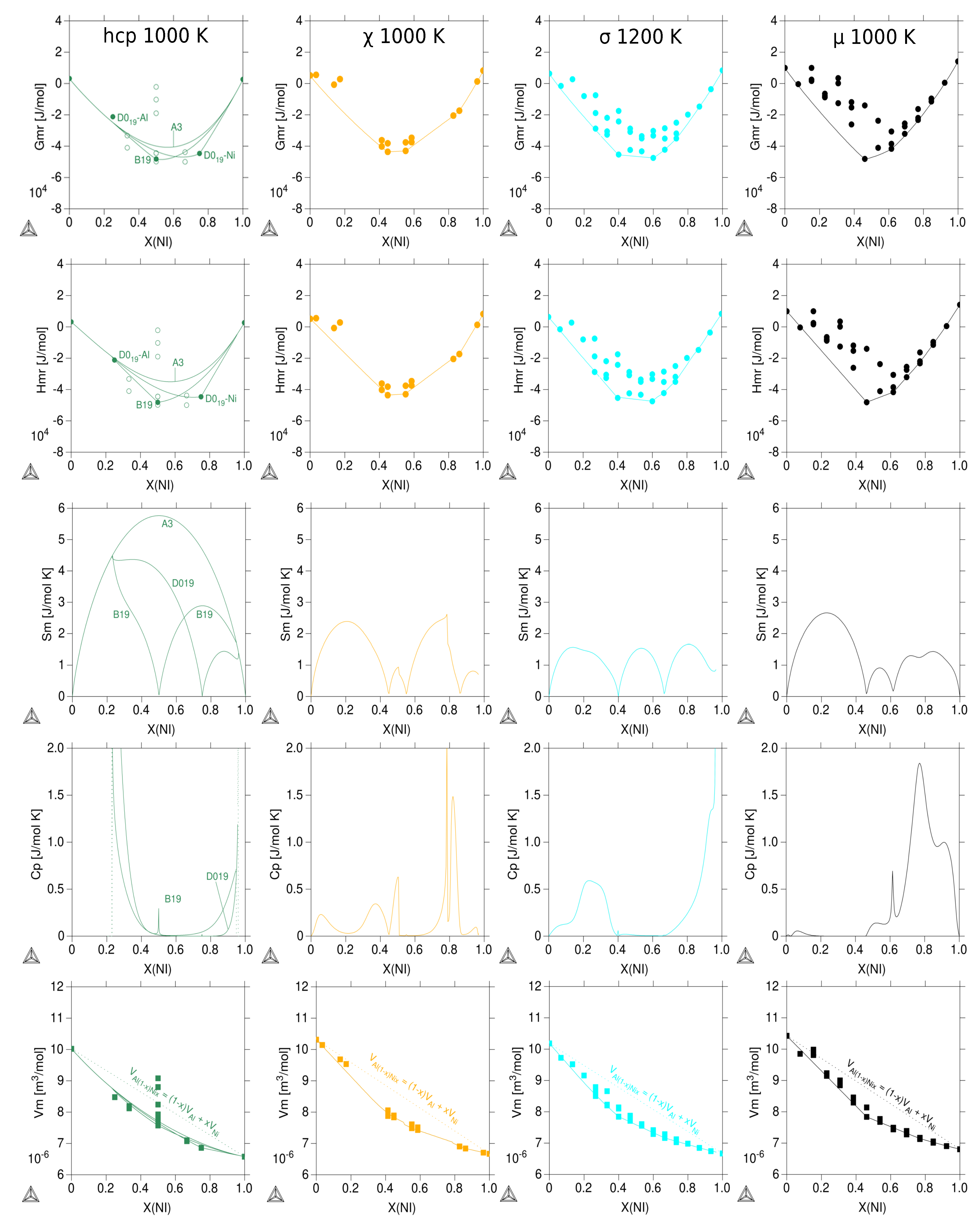
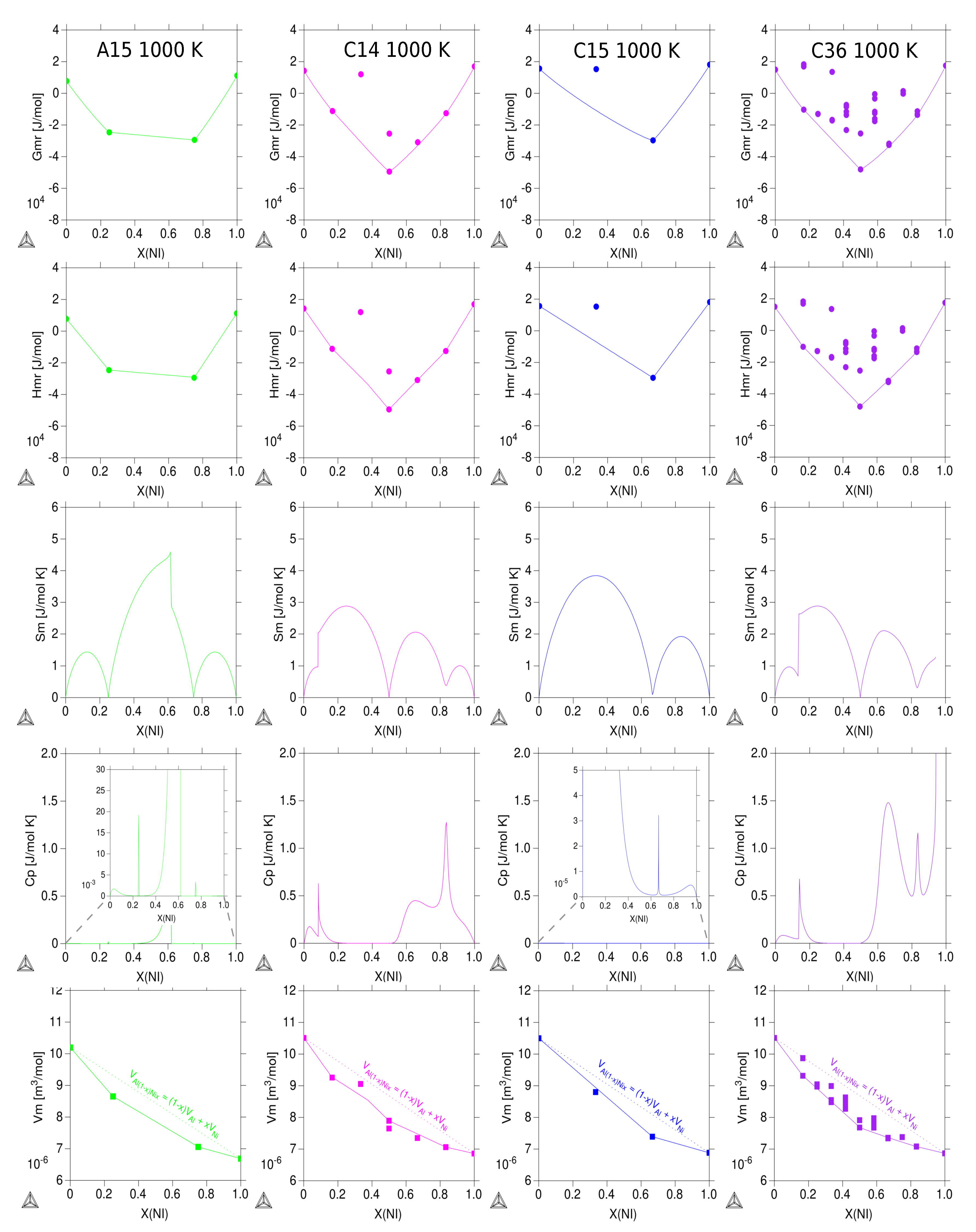
3.3. Thermodynamic Properties of Individual Phases at Finite Temperature

The thermodynamic properties of individual phases of Al–Ni at finite temperatures were calculated using the Gibbs energy set constructed from the DFT results, as described in Section 2.2. The resulting configurational Gibbs energy, enthalpy, entropy, heat capacity and molar volume are presented in Figure 4, Figure 5 and Figure 6 for each phase at 1000 K. Stable phases in the Al–Ni system are grouped in Figure 4 and metastable ones in Figure 5 and Figure 6.

The 4SL model used for fcc and bcc solid solutions allows us to calculate separately the configurational free energies of the different order possibilities (variants). In Figure 4 columns correspond to different phases and rows to thermodynamic properties. The first column corresponds to the fcc family described with 4SL. It shows the completely disordered case A1 where all sublattices have the same site fractions ($y_i^{\left(1\right)}$ = $y_i^{\left(2\right)}$ = $y_i^{\left(3\right)}$ = $y_i^{\left(4\right)}$), the two L1${}_2$ where only three SLs have the same occupation (e.g., $y_i^{\left(1\right)}$ = $y_i^{\left(2\right)}$ = $y_i^{\left(3\right)}\ne y_i^{\left(4\right)}$) identified as L1${}_2$-Al for Al-rich and L1${}_2$-Ni for Ni-rich. L1${}_2$-Al is not very stable but it is slightly ordered at 1000 K and it can be observed in the plot of the Gibbs energy just below A1. Continuing with the rest of the fcc orderings, when two SLs have the same site fraction but different from the other two (e.g., $y_i^{\left(1\right)}$ = $y_i^{\left(2\right)}\ne y_i^{\left(3\right)}$ = $y_i^{\left(4\right)}$), the curves are identified as L1${}_0$, and when two SLs have the same site occupancy but the two other are different (e.g. $y_i^{\left(1\right)}$ = $y_i^{\left(2\right)}\ne y_i^{\left(3\right)}\ne y_i^{\left(4\right)}$) we obtain the L${}^{\prime }$ ordering. L${}^{\prime }$ appears as a mixture between L1${}_0$ and L1${}_2$ and has a second order transformation with L1${}_0$. The L${}^{\prime }$ phase was initially reported in the work of Shockley [48] ($\zeta$ phase), was confirmed later on by the cluster variation [49] and Monte Carlo [50] methods and more recently was found experimentally in epitaxial films [51]. The Gibbs energies of the completely disordered and the most stable fcc based phases at 1000 K were calculated as a function of composition. The differences between the curves for the ordered phases and the disordered phase represent the energy required to bring one mole of an ordered alloy to complete disorder at the temperature of the calculation. Similar interpretation applies for the bcc and hcp solution phases.

The second row of Figure 4 shows the enthalpy as a function of composition. In the first column, it is interesting to understand that the enthalpy of mixing of the disordered phase A1 is calculated from the DFT energies for the three fully ordered structures corresponding to the L1${}_2$-Al${}_3$Ni, L1${}_0$-AlNi and L1${}_2$-AlNi${}_3$ (L1${}_2$-B3A, L1${}_0$-AB and L1${}_2$-A3B in Table 3) and not from an interaction energy dependent on composition as in the Redlich–Kister formalism usually used in the Calphad approach when treating substitutional solutions. Similarly, in the second column, the bcc disordered state description is based on the DFT results for the D0${}_3$-Al${}_3$Ni, B2-AlNi, B32-AlNi and D0${}_3$-AlNi${}_3$.

The third row shows the configurational entropy and the different orderings are labeled accordingly. The entropy shows a sharp minima at the ideal ordering composition; the slight order-tendency of the L1${}_2$-Al mentioned before can also be observed in the configurational entropy.

Continuing, in the fourth row the configurational heat capacity is presented as a function of composition. The shape of the curve was first identified by Kusoffsky and Sundman [52] in a generic system A-B and later on in the fcc alloys of the Al–Ni system [53]. The most noticeable features of the curve shape are the peaks and wings around stoichiometric compositions. In our case the heat capacities of the solid solutions A1, A2 and A3 are zero since there is no heat capacity description for the pure elements. Our results evidence the asymmetry of the real system which can also be observed in [53] but cannot be observed in a prototype A-B system [52], and for the same reason the L1${}_2$-Al and L${}^{\prime }$-Al phases are hard to stabilize in the Al-rich region. However, we were able to calculate the L${}^{\prime }$-Ni ordering in the Ni-rich side; it has no ideal ordering composition but does have a minimum in the heat capacity between the ideal ordering of L1${}_0$ and L1${}_2$, i.e., 50 and 75 at.% Ni. The previously mentioned second-order transition to L1${}_0$ is indicated with a long-dashed line, whereas the dotted line represents two-phase regions.

Finally, in the last row the calculated DFT-CEF molar volumes are shown for each phase in the whole composition range. The departure from Zen’s law of the calculated volume represented here is due to the use of the volume obtained by DFT for each configuration included in the database and not to the use of any excess parameters. The circle-symbols represent the DFT energies and squares DFT volumes, while full and empty symbols represent included and not included in the TDB, respectively.

In the same figure, it is possible to compare fcc and bcc phases with D0${}_{11}$ and D5${}_{13}$ and the main difference can be observed in the configurational entropy, where higher values indicate the higher degree of disorder for the solution phases with respect to D0${}_{11}$ and D5${}_{13}$—stoichiometric and with a narrow homogeneity range for their experimental compositions, respectively. Hence, it is worth noticing the calculated Gibbs energies for D0${}_{11}$ and D5${}_{13}$ in the whole composition range. This description of the Gibbs energy is important for diffusion and phase-field models that explore regions where experiments are not possible as the phase is not observable experimentally.

Figure 5 shows the thermodynamic properties for phases of technological interest such as $\sigma$ and $\mu$ that can precipitate in multicomponent systems, such as Ni-based superalloys, that are based on Al–Ni. The hcp solution phase was also grouped in this figure as it is metastable in this system. Similar interpretations as the above described apply here as well. Only for the $\sigma$ phase was the selected temperature 1200 K due to convergence issues at lower temperatures. Likewise, in Figure 6 the results for A15 and Laves phases are presented together with the DFT formation energies of the end-members at 0 K. These calculations allow one to model driving forces for phase stabilization of important phases in higher order systems, such as the Laves C14 that form in the Al–Ni-related systems, Al–Ni-Ti, Al–Ni-Ta and Al–Ni-Nb as the ternary phase.

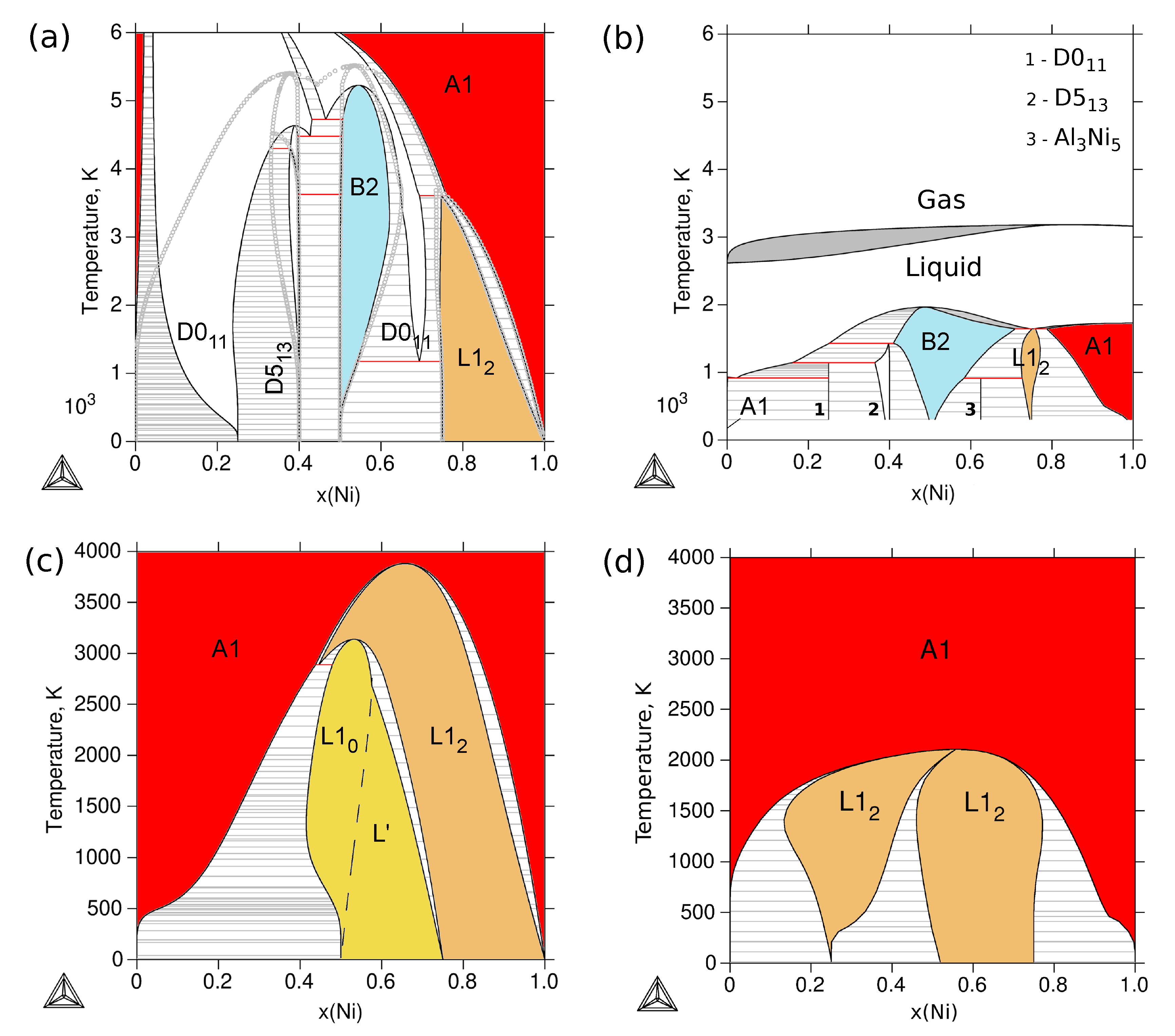
3.4. Phase Stability at Finite Temperature—The Phase Diagram

The DFT-CEF equilibrium diagram for Al–Ni is presented in Figure 7a. It was calculated by combining the formation energies at 0 K from our DFT calculations with the BWG approximation for the configurational entropy in the CEF model, as described in Section 2. The equilibrium calculation included the formation energies for all configurations of Table 4, and for phases with order–disorder transitions, such as fcc, bcc and hcp, the shadowed configurations of Table 3 were used. For the latter the number of end-members was limited to the 4SL model, as implemented in Thermo-Calc using the "F/B" option (the symmetry of the phase was taken into account using the F option after the name of the phase, allowing us to enter equivalent parameters only once in the thermodynamic database): L1${}_2$-AB3, L1${}_0$-AB and L1${}_2$-A3B for fcc; D0${}_3$-AB3, B32, B2 and D0${}_3$-A3B for bcc; and D0${}_{19}$-AB3, hcp-AB and D0${}_{19}$-A3B for hcp phase (see the TDB file in Supplementary Materials). In Figure 7a, the ordered fcc phases are colored red (A1), yellow (L1${}_0$, L${}^{\prime }$) and orange (L1${}_2$), and the ordered bcc phases are colored with light blue. The light-gray symbols superimposed to the equilibrium diagram represent a metastable diagram calculated by suspending the phase D0${}_{11}$ to show how the fcc-A1 equilibrates with D5${}_{13}$ and B2 at high temperatures. D0${}_{11}$-Al${}_3$Ni is experimentally stoichiometric, however, when it is modeled with a 3SL model, such as (Al,Ni)${}_4$(Al,Ni)${}_4$(Al,Ni)${}_8$: using the DFT end-members it shows a significant homogeneity range at finite temperature, while at 0 K shows the correct stoichiometry. D0${}_{11}$ stabilizes in regions where the liquid and Al${}_3$Ni${}_5$ are competing phase, but was not included in the present work.

Several paths to improve the description of the D0${}_{11}$ at finite temperatures can be suggested. In the current approximation, the Gibbs energies of the end-members were only modeled using DFT energies of formation at 0 K. The effects of the phonons were thus neglected, or more exactly, the difference of vibrations between the different phases were neglected. The D0${}_{11}$ is less compact (cf. Figure 2) than the other stable phases and could show significantly different vibrational behavior. Another explanation could come from the use of the BWG approximation. Repulsive excess interaction parameters to account for the interactions between the atoms belonging to the same Wyckoff position could be needed to keep the phase stoichiometric. This feature will be demonstrated in the following for the case of the ordered fcc phases.

For comparison, the critically assessed equilibrium diagram of Al–Ni is presented in Figure 7b—calculated with the TCNI9 database of Thermo-Calc [12]. It is remarkable from Figure 7a that the correct set of stable phases is predicted at low and intermediate temperatures even when metastable phases are entered in the calculation. However, some differences deserve discussion. One of the important differences is the missing homogeneity range of the B2 phase towards the Al rich range. Experimentally this feature has been shown to be due to the presence of vacant sites [54] which are beyond the scope of this work.

A technologically very important region of stability is the two-phase region L1${}_2$/A1 in Figure 7a, the so-called $\gamma$/${\gamma }^{\prime }$ two-phase region. Typical multicomponent alloy processing requires careful control of the composition in order to avoid the precipitation of TCP phases in the coherent $\gamma$/${\gamma }^{\prime }$ matrix in detriment to the alloy properties. The predicted L1${}_2$/A1 stability range is not fully in agreement with the accepted equilibrium diagram and it also shows a wide range of non-stoichiometry for L1${}_2$ at 0 K (cf. Figure 7a,b). The range of non-stoichiometry at 0 K can also be observed in the calculated fcc metastable phase diagrams in Figure 7c, not only for L1${}_2$ but also for L1${}_0$. Figure 7d shows the metastable fcc diagram using the TCNI9 database for comparison, yet a more distinctive feature here is the absence of L1${}_0$ when using the Thermo-Calc database. The reason is that the fcc phase was modeled in this work with a 4SL model, allowing the description of L1${}_0$ and L${}^{\prime }$ orderings, whereas the Thermo-Calc database TCNI9 contains a 2SL model for fcc.

Our DFT equilibrium diagram in Figure 7a can be compared with the work of Goiri et al. [9] where the Al–Ni phase diagram was calculated using DFT energies, cluster expansion and Monte Carlo methods. Although the equilibrium diagram below 600 ${}^{\circ }$C is not shown in their publication, the authors obtained the correct tendency down to 0 K for equilibrium calculations taking into account only ordered fcc and bcc phases of Al–Ni [9,55].

The incorrect tendency of the L1${}_2$ and L1${}_0$ phases at lower temperatures indicates that more ordered fcc structures are needed to properly converge to the ideal stoichiometry at 0 K. However, in order to include more structures from the ones listed in Table 3, a model with more SLs is needed, since with four SLs, structures such as D0${}_{22}$ or D0${}_{23}$, can not be described.

We investigated the possibility of including an excess term, i.e., an interaction parameter, to overcome the above-mentioned limitation of the 4SL model. In order to correct the predicted range of non-stoichiometry at 0 K for the fcc phase, we modified the Gibbs energy, including one excess term, namely, ${}^{L{1}_2}{L}_{Al,Ni:\ast :\ast :\ast }^0=+5000$ J/mol. This is a regular parameter that accounts for the interaction of constituents in the same SL, independent of the occupation of all other SL, as indicated by asterisk, *. In Figure 8a the metastable fcc diagram without excess parameters is shown for comparison with the one including the excess term on the fcc phase, Figure 8b, where the convergence of the phases to the correct stoichiometry at 0 K is shown. Furthermore, Figure 8c shows the corresponding calculated Gibbs energies for the fcc phase at 1000 K without interaction parameter (dashed-red line) and with ${}^{L{1}_2}{L}_{Al,Ni:\ast :\ast :\ast }^0=+5000$ J/mol (solid-black line). The effects of the regular interaction parameter can be clearly seen in the Gibbs energy curves; the major effect is the destabilization of the A1 fully disorder solution. That explains the widening of the two phase fields A1/L1${}_2$ and A1/L1${}_0$ and the increase of the ordering temperatures. The effect is not so drastic on the Gibbs energies of the ordered phases, L1${}_0$ and L1${}_2$, but enough to significantly widen the L1${}_2$/L1${}_0$ field at a low temperature.

4. Conclusions

The phase stability in the Al–Ni system was investigated using a DFT-CEF approach for the whole range of compositions. The formation energies of ordered fcc, bcc and hcp phases, along with D0${}_{11}$, D5${}_{13}$ and the topologically close-packed (TCP) phases $\sigma$, $\mu$, $\chi$, A15, C14, C15 and C36 were obtained by DFT calculations with full chemical permutation on the respective Wyckoff sites. The volumes obtained by the DFT calculations as a function of composition show a fairly linear variation of volume with chemical composition. This provides a significant contribution to the modeling of molar volumes within the Calphad approach.

Using the DFT results, the individual phases were modeled with a complete sublattice description closely related to their crystallographic structure. In particular, the ordered fcc, bcc and hcp phases were modeled with a 4SL model and particular improvements were identified for the fcc phase. The other phases were modeled with one sublattice per Wyckoff site. This combined modeling approach led to good predictions of the phase diagram and the thermodynamic properties at low and intermediate temperatures. The limitations of the applied BWG approximation at high temperatures highlight the importance of further improvements, such as the consideration of further contributions to the free energy and the improvement of the underlying thermodynamic models.

References

1. Fries, S.G.; Lukas, H.L.; Ansara, I.; Sundman, B. The Bragg-Williams-Gorsky (BWG) ordering treatment in the compound energy formalism (CEF). Berichte Der Bunsenges. Für Phys. Chem. 1998, 102, 1102–1110. [Google Scholar] [CrossRef]
2. Lukas, H.; Fries, S.G.; Sundman, B. Computational Thermodynamics. The Calphad Method; Cambridge University Press: Cambridge, UK, 2007. [Google Scholar]
3. Martin, R. Electronic Structure. Basic Theory and Practical Methods; Cambridge University Press: Urbana, IL, USA; Champaign, IL, USA, 2004. [Google Scholar]
4. Dupin, N.; Kattner, U.R.; Sundman, B.; Palumbo, M.; Fries, S.G. Implementation of an Effective Bond Energy Formalism in the Multicomponent Calphad Approach. J. Res. Natl. Inst. Stand. Technol. 2018, 123, 123020. [Google Scholar] [CrossRef]
5. Reed, R.C. The Superalloys; Cambridge University Press: Cambridge, UK, 2006. [Google Scholar]
6. Dupin, N.; Sundman, B. A thermodynamic database for Ni-base superalloys. Scand. J. Metall. 2001, 30, 184–192. [Google Scholar] [CrossRef]
7. Parsa, A.B.; Wollgramm, P.; Buck, H.; Somsen, C.; Kostka, A.; Povstugar, I.; Choi, P.P.; Raabe, D.; Dlouhy, A.; Müller, J.; et al. Advanced scale bridging microstructure analysis of single crystal Ni-base superalloys. Adv. Eng. Mater. 2015, 17, 216–230. [Google Scholar] [CrossRef]
8. Lopez-Galilea, I.; Koßmann, J.; Kostka, A.; Drautz, R.; Mujica Roncery, L.; Hammerschmidt, T.; Huth, S.; Theisen, W. The thermal stability of topologically close-packed phases in the single-crystal Ni-base superalloy ERBO/1. J. Mater. Sci. 2016, 51, 2653–2664. [Google Scholar] [CrossRef]
9. Goiri, J.G.; Van Der Ven, A. Phase and structural stability in Ni-Al systems from first principles. Phys. Rev. B 2016, 94, 16–19. [Google Scholar] [CrossRef] [Green Version]
10. Palumbo, M.; Fries, S.G.; Hammerschmidt, T.; Abe, T.; Crivello, J.C.; Breidi, A.A.H.; Joubert, J.M.; Drautz, R. First-principles-based phase diagrams and thermodynamic properties of TCP phases in Re–X systems (X = Ta, V, W). Comput. Mater. Sci. 2014, 81, 433–445. [Google Scholar] [CrossRef]
11. Andersson, J.O.; Helander, T.; Höglund, L.; Shi, P.; Sundman, B. Thermo-Calc & DICTRA, computational tools for materials science. Calphad 2002, 26, 273–312. [Google Scholar]
12. Thermo-Calc. Available online: http://www.thermocalc.com (accessed on 17 June 2020).
13. van de Walle, A.; Sun, R.; Hong, Q.J.; Kadkhodaei, S. Software tools for high-throughput CALPHAD from first-principles data. Calphad 2017, 58, 70–81. [Google Scholar] [CrossRef]
14. Wang, P.; Koßmann, J.; Kattner, U.R.; Palumbo, M.; Hammerschmidt, T.; Olson, G.B. Thermodynamic assessment of the Co-Ta system. Calphad 2019, 64, 205–212. [Google Scholar] [CrossRef]
15. Kresse, G.; Hafner, J. Ab initio molecular dynamics for liquid metals. Phys. Rev. B 1993, 47, 558–561. [Google Scholar] [CrossRef] [PubMed]
16. Kresse, G.; Furthmüller, J. Efficiency of ab-initio total energy calculations for metals and semiconductors using a plane-wave basis set. Comput. Mater. Sci. 1996, 6, 15–50. [Google Scholar] [CrossRef]
17. Kresse, G.; Furthmüller, J. Efficient iterative schemes for ab initio total-energy calculations using a plane-wave basis set. Phys. Rev. B 1996, 54, 11169–11186. [Google Scholar] [CrossRef] [PubMed]
18. Hammerschmidt, T.; Bialon, A.; Pettifor, D.; Drautz, R. Topologically closed-packed phases in binary transition-metal compounds: Matching high-throughput ab-initio calculations to an empirical structure-map. New J. Phys. 2013, 15, 115016. [Google Scholar] [CrossRef]
19. Perdew, J.P.; Burke, K.; Ernzerhof, M. Generalized Gradient Approximation Made Simple. Phys. Rev. Lett. 1996, 77, 3865–3868. [Google Scholar] [CrossRef] [PubMed] [Green Version]
20. Monkhorst, H.J.; Pack, J.D. Special points for Brillouin-zone integrations. Phys. Rev. B 1976, 13, 5188–5192. [Google Scholar] [CrossRef]
21. Fries, S.G.; Sundman, B. Using Re-W σ-phase first-principles results in the Bragg-Williams approximation to calculate finite-temperature thermodynamic properties. Phys. Rev. B 2002, 66, 012203. [Google Scholar] [CrossRef]
22. Andersson, J.O.; Guillermet, A.; Hillert, M. A compound-energy model of ordering in a phase with sites of different coordination numbers. Acta Metall. 1986, 34, 437–445. [Google Scholar] [CrossRef]
23. Hillert, M. The compound energy formalism. J. Alloys Compd. 2001, 320, 161–176. [Google Scholar] [CrossRef]
24. Sluiter, M. Ab initio lattice stabilities of some elemental complex structures. Calphad 2006, 30, 357–366. [Google Scholar] [CrossRef]
25. Wang, Y.; Curtarolo, S.; Jiang, C.; Arroyave, R.; Wang, T.; Ceder, G.; Chen, L.Q.; Liu, Z.K. Ab initio lattice stability in comparison with CALPHAD lattice stability. Calphad 2004, 28, 79–90. [Google Scholar] [CrossRef]
26. Dinsdale, A.T. SGTE data for pure elements. Calphad 1991, 15, 317–425. [Google Scholar] [CrossRef]
27. Palumbo, M.; ICAMS–RUB, Bochum, Germany. Personal communication. 2015–2016.
28. Sin’ko, G.V.; Smirnov, N.A. Ab initio calculations of elastic constants and thermodynamic properties of bcc, fcc, and hcp Al crystals under pressure. J. Phys. Condens. Matter 2002, 14, 6989–7005. [Google Scholar]
29. Lu, Z.W.; Wei, S.H.H.; Zunger, A.; Frota-Pessoa, S.; Ferreira, L.G. First-principles statistical mechanics of structural stability of intermetallic compounds. Phys. Rev. B 1991, 44, 512–544. [Google Scholar] [CrossRef] [Green Version]
30. Yan, J.Y.; Olson, G.B. Molar volumes of bcc, hcp, and orthorhombic Ti-base solid solutions at room temperature. Calphad 2016, 52, 152–158. [Google Scholar] [CrossRef] [Green Version]
31. Hallstedt, B. Molar volumes of Al, Li, Mg and Si. Calphad 2007, 31, 292–302. [Google Scholar] [CrossRef]
32. Syassen, K.; Holzapfel, W.B. Isothermal compression of Al and Ag to 120 kbar. J. Appl. Phys. 1978, 49, 4427–4430. [Google Scholar] [CrossRef]
33. Palumbo, M.; Fries, S.G.; Dal Corso, A.; Körmann, F.; Hickel, T.; Neugebauer, J. Reliability evaluation of thermophysical properties from first-principles calculations. J. Phys. Condens. Matter 2014, 26, 335401. [Google Scholar] [CrossRef]
34. Rasamny, M.; Weinert, M.; Fernando, G.W.; Watson, R.E. Electronic structure of a neutral oxygen vacancy in Al3Ni. Phys. Rev. B 2001, 64, 144107. [Google Scholar] [CrossRef]
35. Saniz, R.; Ye, L.H.; Shishidou, T.; Freeman, A.J. Structural, electronic, and optical properties of Al3Ni: First-principles calculations. Phys. Rev. B 2006, 74, 014209. [Google Scholar] [CrossRef] [Green Version]
36. Chrifi-Alaoui, F.; Nassik, M.; Mahdouk, K.; Gachon, J. Enthalpies of formation of the Al–Ni intermetallic compounds. J. Alloys Compd. 2004, 364, 121–126. [Google Scholar] [CrossRef]
37. Grimvall, G. Reconciling ab initio and semiempirical approaches to lattice stabilities. Berichte Der Bunsenges. Für Phys. Chem. 1998, 102, 1083–1087. [Google Scholar] [CrossRef]
38. Burton, B.P.; Dupin, N.; Fries, S.G.; Grimvall, G.; Fernandez-Guillermet, A.; Miodownik, P.; Oates, W.A.; Vinograd, V. Using Abinitio calculations in the Calphad enviroment. Z. Für Metallkunde. 2001, 92, 514–525. [Google Scholar]
39. Lu, X.; Selleby, M.; Sundman, B. Theoretical modeling of molar volume and thermal expansion. Acta Mater. 2005, 53, 2259–2272. [Google Scholar] [CrossRef] [Green Version]
40. Zhang, B.; Li, X.; Li, D. Assessment of thermal expansion coefficient for pure metals. Calphad 2013, 43, 7–17. [Google Scholar] [CrossRef]
41. Kaptay, G. Approximated equations for molar volumes of pure solid fcc metals and their liquids from zero Kelvin to above their melting points at standard pressure. J. Mater. Sci. 2015, 50, 678–687. [Google Scholar] [CrossRef]
42. Vegard, Y.L. Yon Lo Vegard. Z. Für Phys. 1921, 5, 17–26. [Google Scholar] [CrossRef]
43. Hafner, J. A note on Vegard’s and Zen’s laws. J. Phys. F Met. Phys. 1985, 15, 43–48. [Google Scholar] [CrossRef]
44. Materials Project. Available online: https://www.materialsproject.org (accessed on 17 June 2020).
45. Pearson, W.B. A Handbook of Lattice Spacings and Structures of Metals and Alloys, International Series of Monographs on Metal Physics and Physical Metallurgy Volume 4; Pergamon Press: Oxford, UK, 1958. [Google Scholar]
46. Ellner, M.; Kattner, U.; Predel, B. Konstitutionelle und strukturelle untersuchungen im aluminiumreichen teil der systeme Ni-Al und Pt-Al. J. Less-Common Met. 1982, 87, 305–325. [Google Scholar] [CrossRef]
47. Taylor, A.; Doyle, N.J. Further Studies on the Ni-Al System. I. The beta-NiAI and delta Ni2Al3 phase fields. J. Appl. Crystallogr. 1972, 5, 201. [Google Scholar] [CrossRef]
48. Shockley, W. Theory of order for the copper gold alloy system. J. Chem. Phys. 1938, 6, 130–144. [Google Scholar] [CrossRef]
49. Finel, A.; Ducastelle, F. On the phase diagram of the fcc ising model with antiferromagnetic first-neighbour interactions. Europhys. Lett. 1986, 1, 135–140. [Google Scholar] [CrossRef]
50. Tétot, R.; Finel, A.; Ducastelle, F. Superdegenerate point in FCC phase diagram: CVM and Monte Carlo investigations. J. Stat. Phys. 1990, 61, 121–141. [Google Scholar] [CrossRef]
51. Steiner, M.A.; Comes, R.B.; Floro, J.A.; Soffa, W.A.; Fitz-Gerald, J.M. L1 ordering: Evidence of L10-L12 hybridization in strained Fe38.5Pd61.5 epitaxial films. Acta Mater. 2015, 85, 261–269. [Google Scholar] [CrossRef]
52. Kusoffsky, A.; Sundman, B. Irregular Composition-Dependence of the Configurational Heat Capacity in the Modelling of Ordered Alloys. J. Phys. Chem. Solids 1998, 59, 1549–1553. [Google Scholar] [CrossRef]
53. Geng, H.Y.; Sluiter, M.H.F.; Chen, N.X. Order-disorder effects on the equation of state for fcc Ni-Al alloys. Phys. Rev. B 2005, 72, 014204. [Google Scholar] [CrossRef] [Green Version]
54. Bradley, A.J.; Taylor, A. An X-Ray Analysis of the Nickel-Aluminium System. Proc. R. Soc. Lond. A 1937, 159, 56–72. [Google Scholar]
55. Van Der Ven, A.; Materials Department, University of California, Santa Barbara, CA, USA. Personal communication, 2019.
Figure 1. Formation energy of ordered Al–Ni compounds at 0 K with respect to the Al and Ni ground-state structure as obtained by DFT. The straight lines indicate the convex hulls of the individual phases as a function of composition. The dashed line defines the overall structural stability.
Metals 10 01142 g001
Figure 2. Molar volumes of stable and metastable ordered Al–Ni phases at 0 K as obtained from DFT calculations.
Metals 10 01142 g002
Figure 3. Molar volumes at 0 K as obtained by DFT compared with Zen’s law (dashed line) and fitted using a regular solution model V m ϕ (dashdotted line) for ordered compounds of fcc, bcc, D0 11 -Al 3 Ni and D5 13 -Al 3 Ni 2 . Values from the literature were calculated: 91Lu [29] with three different methods; Vm1 (LMTO), Vm2 and Vm3 (CE); and mp-AlNi 3 , mp-B2 and mp-Al 3 Ni 2 from the materials project database [44]; experimental: 82Ell [46] and 72Tay [47].
Metals 10 01142 g003
Figure 4. Calculated thermodynamic properties at 1000 K for fcc, bcc, D0 11 and D5 13 phases using Thermo-Calc v.2020a and the assembled DFT-Calphad database. The circles represent the DFT formation energies at 0 K for the ordered compounds; full and empty indicate included and not in the assembled TDB, respectively.
Metals 10 01142 g004
Figure 5. Calculated thermodynamic properties at 1000 K for metastable: hcp, χ , σ and μ phases in the whole composition range using Thermo-Calc v.2020a and the assembled DFT-Calphad database. The dots represent the DFT formation energies at 0 K for the ordered compounds.
Metals 10 01142 g005
Figure 6. Calculated thermodynamic properties at 1000 K for A15, C14, C15 and C36 phases using Thermo-Calc v.2020a and the assembled DFT-Calphad database. The dots represent the DFT formation energies at 0 K for the ordered compounds.
Metals 10 01142 g006
Figure 7. Calculated Al–Ni phase diagrams using Thermo-Calc v.2020a. (a) Equilibrium predicted using the assembled DFT-CEF database. (b) Equilibrium calculated using Thermo-Calc proprietary database TCNI9. (c) Metastable fcc predicted using the assembled DFT-CEF database. (d) Metastable fcc calculated using TCNI9.
Metals 10 01142 g007
Figure 8. Al–Ni calculated DFT-CEF metastable diagrams with a regular parameter (a) L 1 2 L A l , N i : : : 0 = 0 J/mol and (b) L 1 2 L A l , N i : : : 0 = + 5000 J/mol. (c) Gibbs energy curves with reference to fcc-A1 at the actual temperature for the fcc phase with L 1 2 L A l , N i : : : 0 = 0 J/mol (dashed red line) and L 1 2 L A l , N i : : : 0 = + 5000 J/mol (solid black line).
Metals 10 01142 g008