An Improved Johnson–Cook Constitutive Model and Its Experiment Validation on Cutting Force of ADC12 Aluminum Alloy During High-Speed Milling

Abstract

Because of the massive work and high cost of milling experiments, finite element analysis technology (FEA) was used to analyze the milling process of ADC12 aluminum alloy. An improved Johnson–Cook (J–C) constitutive equation was fitted by a series of dynamic impact tests in different strain rates and temperatures. It found that the flow stress gradually increases as the strain rate rises, but it decreases as the test temperature rises. Compared with the J–C constitutive model, the predicted flow stress by the improved J–C constitutive model was closer to the experimental results when the strain rate was larger than 8000 s⁻¹ and the temperature was higher than 300 °C. A two-dimensional cycloidal cutting simulation model was constructed based on the two J–C constitutive equations which was validated by milling experiments at different cutting speeds. The simulation results based on the improved J–C constitutive equation were closer to the experimental results and showed the cutting force first increased and then decreased, with cutting speed increasing, reaching a maximum at 600 m/min.

1. Introduction

The ADC12 aluminum alloy has been widely used in engine cylinder bodies and heads with its low density, good casting performance, wear resistance, and small thermal expansion coefficient in recent years [1]. As a kind of Al–Si alloy, this alloy easily undergoes high temperatures in high-speed cutting processes, thus aggravating tool wear [2]. Many researchers have carried out experimental studies on the temperature distribution in the cutting zone affected by the tool crater wear and tool flank wear [3,4,5]. These studies have found that tool wear not only affects the cutting force and cutting temperature, but also affects the machined surface topography. The main methods to measure the tool surface temperature in high-speed milling are thermocouple temperature measurement and infrared temperature measurement [6,7,8]. Many researchers have proposed the theoretical temperature field analytical model [9,10], finite element analysis model, and experimental verification [11,12,13,14,15] to analyze the temperature distribution of the high-speed cutting process. It found that the cutting force, which periodically changes during milling process, will produce higher temperatures at the tool–chip interface, further affecting tool wear and machining surface quality. This is due to the aluminum alloy milling process is a multi-tooth discontinuous cutting process. Therefore, studying the variation of cutting force is helpful to analyze the tool wear behavior during high-speed milling of ADC12 alloy. Because of the massive work and high cost of high-speed milling experiments, it is the trend to study the cutting force during high-speed milling of alloy by finite element analysis technology (FEA).

Fitting a constitutive equation is an essential step before establishing the simulation model of high-speed cutting [16,17]. There are several constitutive equations for metal cutting simulation, including the Johnson–Cook [18], Power–Law [19], and Zerilli–Armstrong [20]. In the Z–A model, the strain hardening coefficient is assumed to be independent of strain rate and temperature, resulting in that all parameters in the model are constant and do not change with the strain rate and temperature which is inconsistent with the actual machining situation. The J–C model and P–L model are both empirical viscoplastic constitutive models with concise form and describe the relationship between stress and strain, strain rate, and temperature. Besides that, the J–C constitutive equation has the most extensive application owing to its obvious physical significance of parameters and suitability for numerical simulation. Researchers proved that the material constants of the J–C constitutive equation have important influence on the finite element simulation model [21,22].

Xu et al. [17] converted the J–C constitutive equation into a function of strain strengthening coefficient, strain rate strengthening coefficient, and thermal softening coefficient to more clearly describe the strain, strain rate, and thermal effects on the flow stress. This theory describes the thermal softening effect by cubic polynomial and describes the strain hardening effect using the second-order polynomial [23,24]. Guo et al. [25] pointed out that strain and strain rate have an effect on temperature owing to the adiabatic deformation at high strain rate. He proposed a general method to characterize flow stress during high-speed cutting by calibrating the J–C constitutive model’s parameters with a quasi-static compression experiment and high-speed cutting experiment. An accurate J–C constitutive model has important influence on the finite element simulation, which not only describes the chip formation process more accurately [26] but also explains the characters of temperature distribution in the cutting zone more specifically [27].

In this study, the true stress–strain curves were obtained by quasi-static experiments and Split Hopkinson Pressure Bar experiments. A J–C constitutive model and an improved J–C constitutive model were fitted according to the experimental results. Through a series of high-speed milling experiments, the simulation model established by the improved J–C constitutive equation was verified. The purpose of this study was to fit a constitutive model of ADC12 alloy for finite element analysis high-speed cutting, so as to research the characteristics of the stress distribution and temperature variation during high-speed cutting and to provide certain reference for studying tool wear and workpiece surface quality.

2. Experimental Procedure

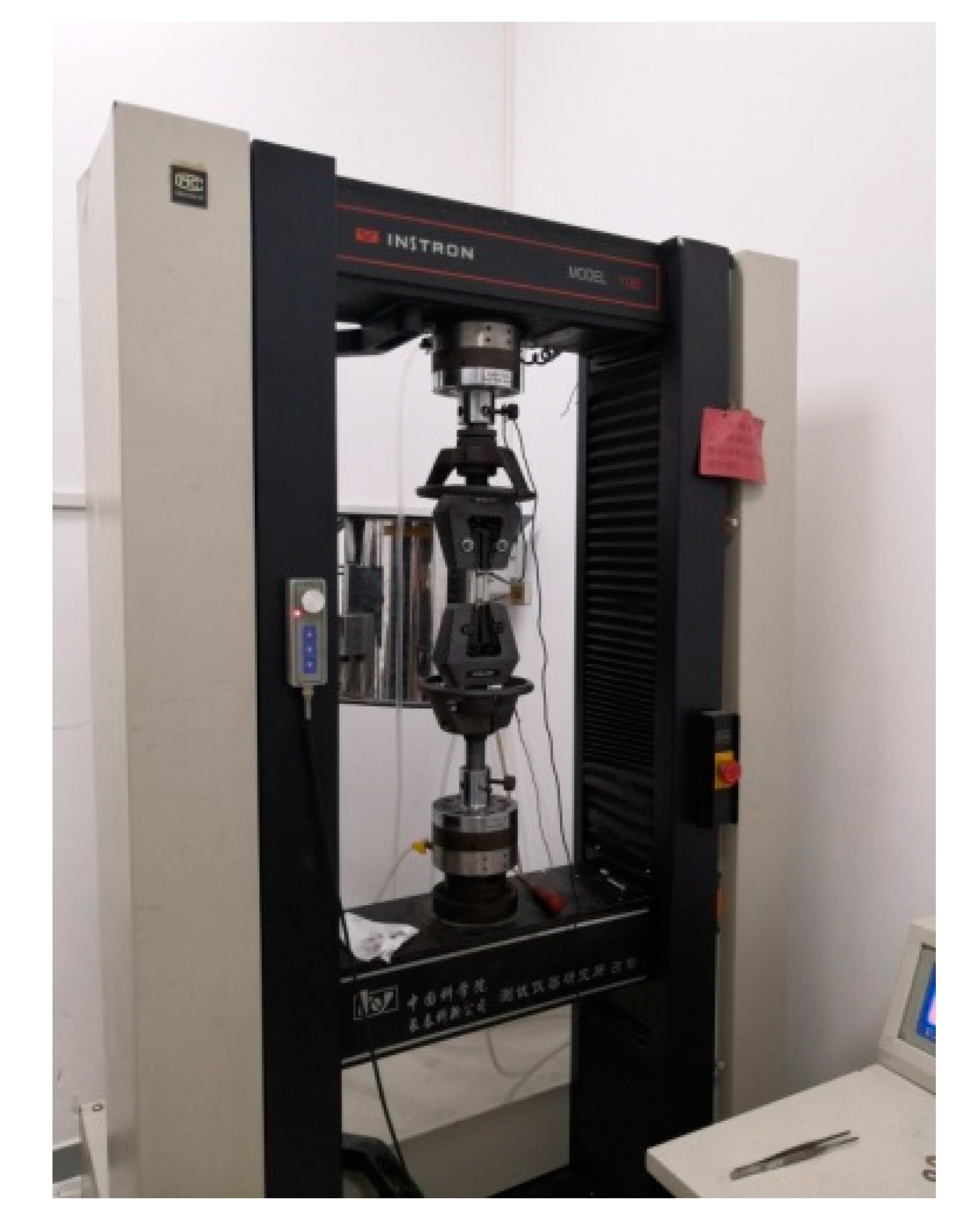
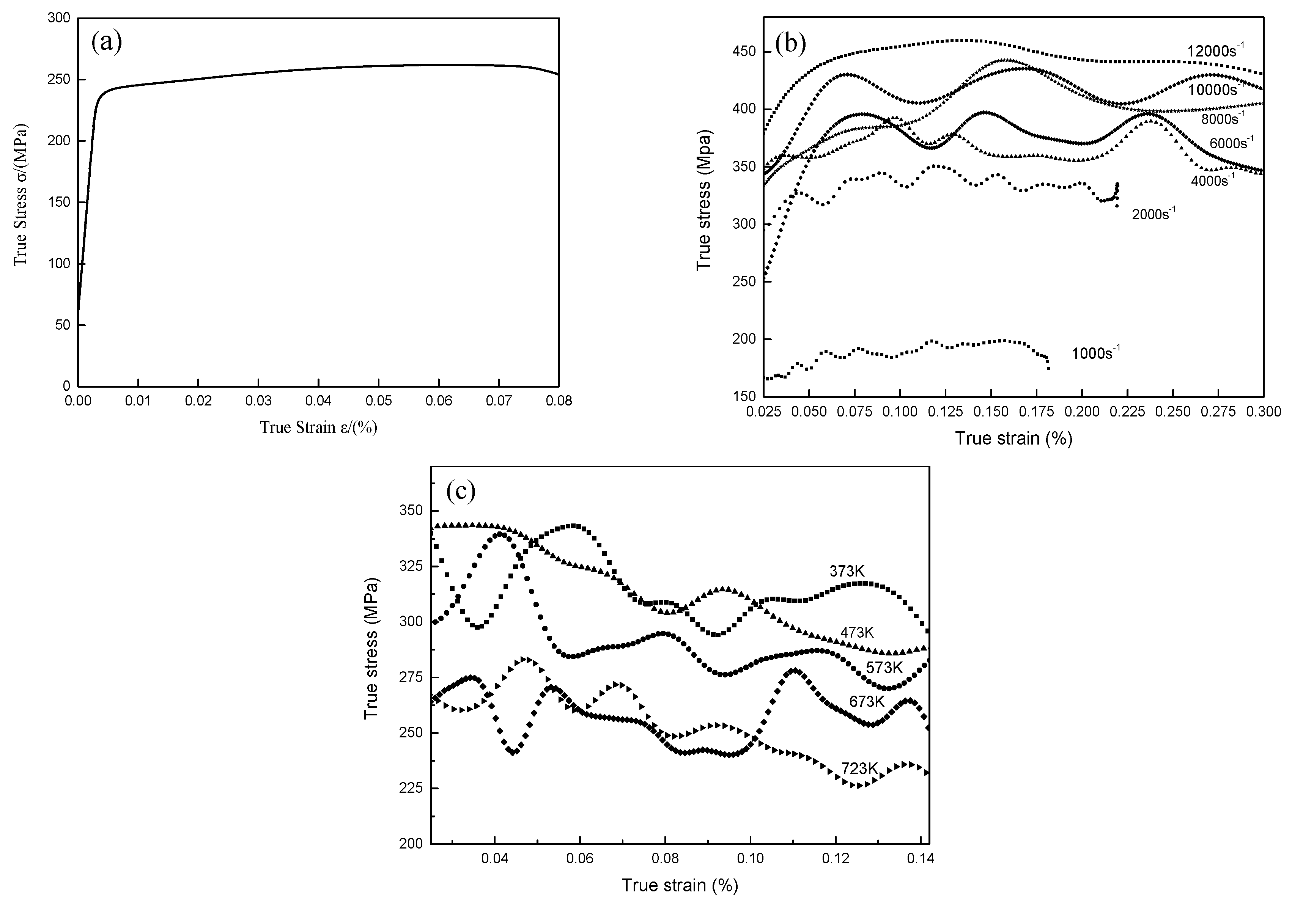
2.1. Quasi-Static Experiments

Table 1. compositions of the ADC12 aluminum alloy.

Chemical Compositions (%)
Si	Fe	Cu	Mg	Mn	Zn	Ni	Sn	Al
9.6–12	<1.3	1.5–3.5	<0.3	<0.5	<1.0	<0.5	≤0.3	others

lists the chemical composition of ADC12 aluminum alloy. The alloy has a hardness of approximately 86 HB and a melting temperature of 580 °C. The quasi-static experiments were performed at the tensile rate of 1 mm/min at room temperature via a universal material testing machine (Instron, High Wycombe, UK). The quasi-static tensile experiment setup is shown in Figure 1. The model of the universal material testing machine was Instron 1185. The cylindrical specimens were φ5 mm × 100 mm. The extensometer gauge length was 50 mm. In addition to the requirements for geometric size, the specimens should have good parallelism and perpendicularity, and which were kept at approximately 0.01 mm and the surface roughness Ra = 1.6 μm. The experiment was repeated three times.

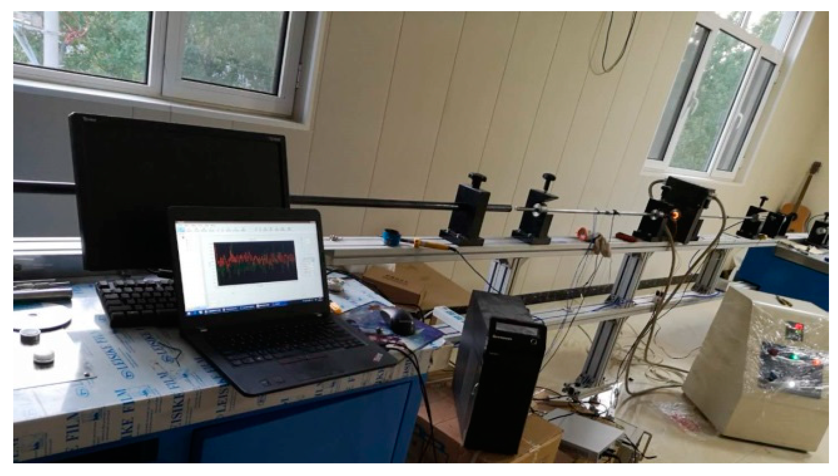
2.2. Split Hopkinson Pressure Bar Experiment

The SHPB tests were performed using the ARCHIMEDES ALT1000 Hopkinson Bar test system (Archimedes Industrial Technology Limited, Hong Kong, China) at strain rates of 1000–12,000 s⁻¹ and at temperatures of 20–450 °C. The pressure bar with a diameter of 15 mm was adopted. The size of the SHPB experiment specimens was φ3 mm × 3 mm. The parallel degree of the specimens’ two end faces was 0.01 mm, and the surface roughness was Ra = 0.8 μm.

Figure 2 presents the SHPB experiment setup. Owing to true strain rates for SHPB tests not being constant, all the experiments were repeated five times. All the experimental results were converted to true stress–strain curves in this work, which are shown in Figure 3a–c. It was found that the flow stress gradually increased with the rise in the strain rate, but this decreased when the test temperature rose. This confirms the effect of strain rate strengthening and thermal softening on the flow stress.

3. Results and Discussion

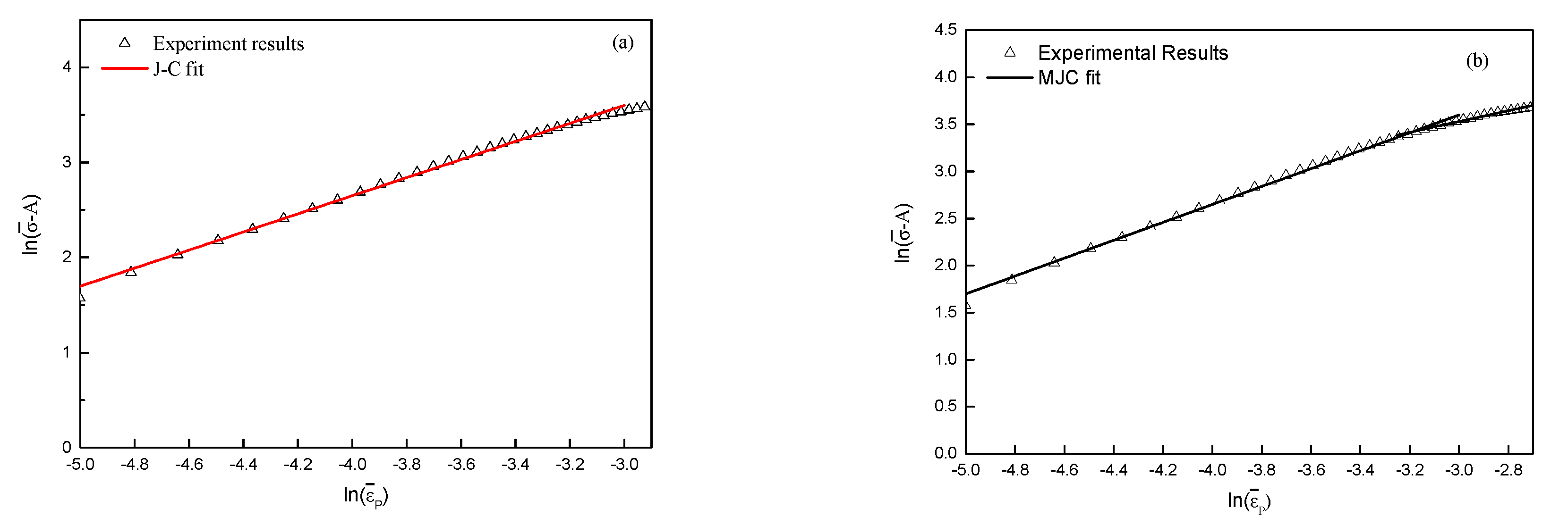
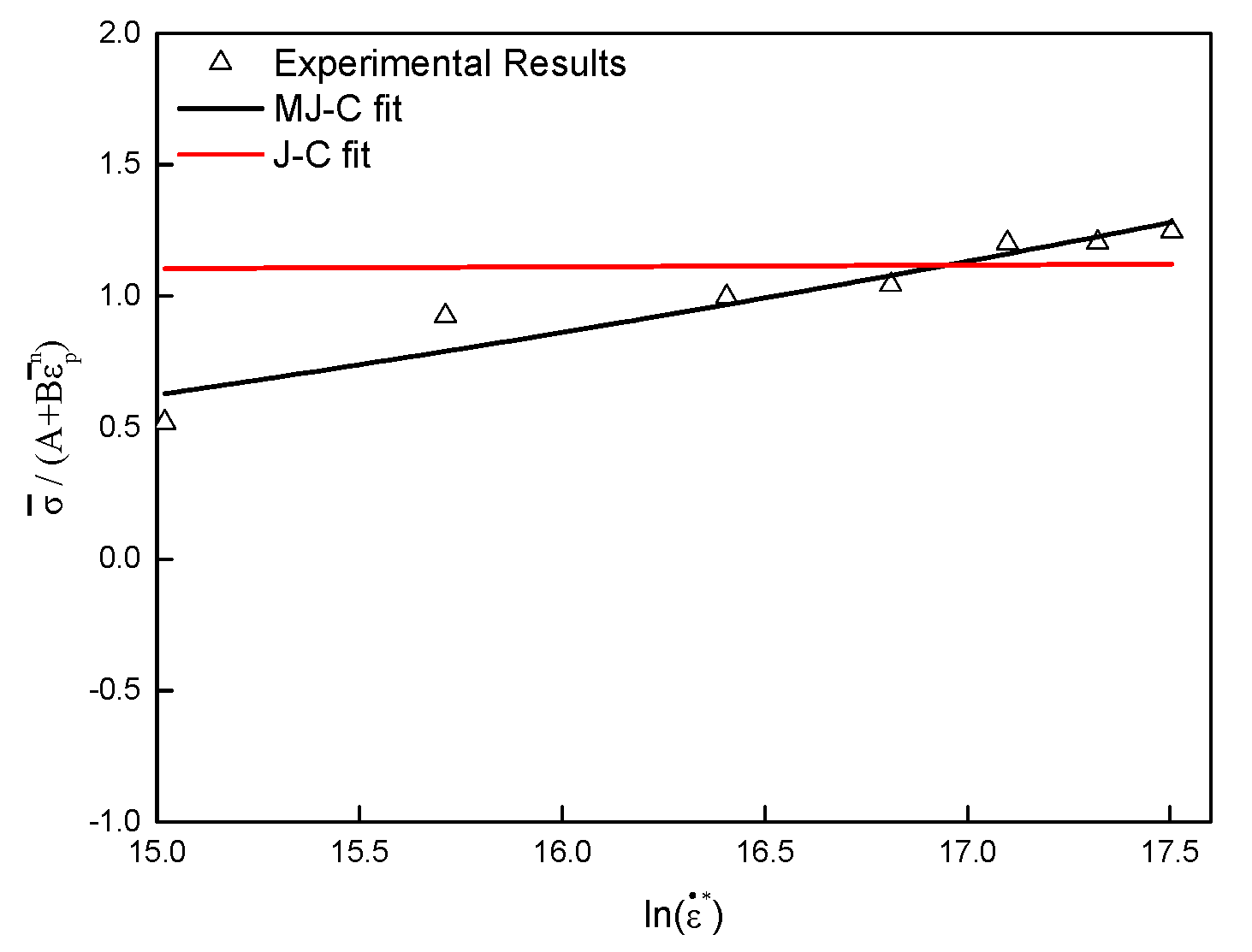
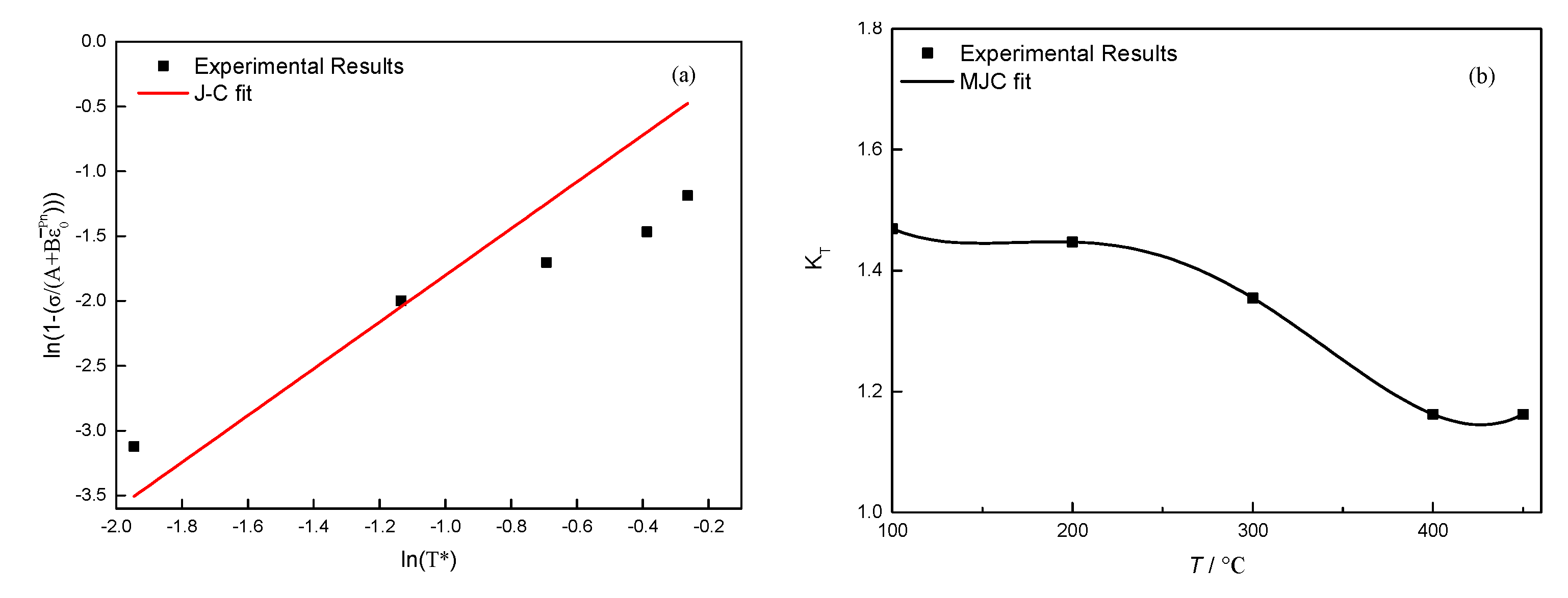
3.1. Improved Johnson–Cook Constitutive Model

The classical Johnson–Cook equation is expressed in Equation (1) [18] which describes the effect of strain ${\epsilon }_P$, strain rate $\stackrel{·}{\epsilon }$ and temperature $T$ on the flow stress $\sigma$. A is the initial yield stress. B and n are the coefficient of strain effect. C and m are the coefficient of strain rate effect and temperature effect. The improved J–C constitutive equation uses $K_{\epsilon }$ to describe the strain effect, $K_{{\epsilon }^{’}}$ to describe the strain rate effect and $K_T$ to describe the temperature effect, as shown in Equation (2).

$$\begin{gathered} \sigma =(A+B{\epsilon }_P^n)(1+Cln{\stackrel{·}{\epsilon }}^{*})(1-T^{*m}) \\ {\stackrel{·}{\epsilon }}^{*}=\frac{\stackrel{·}{\epsilon }}{\stackrel{·}{{\epsilon }_0}},T^{*}=(T-T_0)/(T_{melt}-T_0) \end{gathered}$$

(1)

$$\sigma =A{K}_{\epsilon }{K}_{{\epsilon }^{’}}{K}_T$$

(2)

Since the classical J–C constitutive model assumes that strain hardening, strain rate hardening, and temperature softening effect are independent effects, the values of both the strain rate effect and the temperature effect are 1 when analyzing the influence of strain hardening effect on stress. Equation (3) can be obtained by simplifying the main equation 1, which presents the effect of strain hardening on the flow stress. Take the logarithm of both sides of Equation (3), and the transformed equation is expressed in Equation (4). The relation between $\ln (\overline{\sigma }-\mathrm{A})$ and $\ln ({\overline{\epsilon }}_P)$ is plotted according to the data obtained from the quasi-static experiments, and a linear line is fitted based on the relation, where n and B are calculated from the characteristics of the slope and intercept of the line. The value of the initial yield stress obtained by the quasi-static experiment was 240 MPa. The values of B and n can be calculated to be 636 MPa and 0.95168, respectively.

$$\overline{\sigma }=A+B{\epsilon }_P^n$$

(3)

$$\ln (\overline{\sigma }-\mathrm{A})=\mathrm{n}\ln ({\overline{\epsilon }}_P)+\ln \mathrm{B}$$

(4)

Different from the J–C model, the improved J–C model uses piecewise function to describe the strain effect. Figure 4a,b presents the fit line of the relationship between $\ln (\overline{\sigma }-\mathrm{A})$ and $\ln ({\overline{\epsilon }}_P)$ by the basic J–C model and the modified J–C model. It is obvious that the fitted line using the piecewise function was closer to the experimental results. The strain hardening effect in the modified J–C constitutive model can be expressed in Equation (5).

$$\left\{\begin{array}{l}\sigma =(240+636{\epsilon }^{0.95168}),\ln ({\epsilon }_P)\in (-5,-3.25]\\ \sigma =(240+191{\epsilon }^{0.57396}),\ln ({\epsilon }_P)\in (-3.25,-2.7)\end{array}\right\}$$

(5)

Dividing both sides of Equation (5) by ${\sigma }_S(240 \mathrm{MPa})$, the relationship between the strain hardening effect $K_{\epsilon }$ and strain $\epsilon$ is expressed in Equation (6).

$$K_{\epsilon }=\frac{\sigma }{A}=\left\{\begin{array}{l}(1+2.65{\epsilon }^{0.95168}),\epsilon \in (0.0067,0.039]\\ (1+0.796{\epsilon }^{0.57396}),\epsilon \in (0.039,0.067)\end{array}\right\}$$

(6)

At the reference temperature condition, the value of temperature effect is 1. Equation (7) which represents the strain hardening effect and strain rate effect on flow stress can be obtained by simplifying the original Equation (1). Through the SHPB experiment at room temperature with a strain rates 1000–12,000 s^‒1, C can be calculated to be 0.00698. The improved model describes the strain rate effect by second-order polynomial. To obtain the relationship between the flow stress and the strain rate effect, the experimental flow stress was divided by the predicted stress which was calculated by Equation (6). By fitting the curve, the strain rate effect is expressed in Equation (8). Figure 5 presents the fit line of the relation between $\ln {\stackrel{·}{\epsilon }}^{*}$ and $\sigma /(A+B{\overline{\epsilon }}_P^n)$ at the reference temperature in two models, which illustrates the fit line by second-order polynomial was closer to the experimental results.

$$\frac{\overline{\sigma }}{(A+B{\overline{\epsilon }}_P^n)}=1+C\ln {\stackrel{·}{\epsilon }}^{*}$$

(7)

$$K_{{\epsilon }^{’}}=\frac{\overline{\sigma }}{A{K}_{\epsilon }}=(-0.27108\ln {\stackrel{·}{\epsilon }}^{*}+0.0164{(\ln {\stackrel{·}{\epsilon }}^{*})}^2+1)$$

(8)

Similarly, according to the SHPB experiment at different temperatures at the reference strain rate condition, Equation (9) can be obtained by simplifying the original equation’s strain rate value to 1 and applying the natural logarithm of both sides of the Equation. m can be calculated to be 1.80151. The fit line is shown in Figure 6a.

$$\ln (1-\frac{\sigma }{A+B{\epsilon }^n})=m\ln (T^{*})$$

(9)

Dividing the experimental flow stress by the predicted stress, the value of the thermal softening coefficient $K_T$ can be obtained. Taking the values of $K_T$ when the strain is 0.2, 0.4, 0.6, 0.8, 1.0, and 1.2, the relation curve between thermal softening coefficient $K_T$ and temperature $T$ can be drawn by taking its average value, as shown in Figure 6b. The improved model described the thermal softening effect by fifth-order polynomial function which is expressed in Equation (10):

$$K_T=\frac{\overline{\sigma }}{A{K}_{\epsilon }{K}_{{\epsilon }^{’}}}=1.97074-1.054\times {10}^{(-2)}T+7.52433\times {10}^{(-5)}{T}^2-2.21592\times {10}^{(-7)}{T}^3+2.16767\times {10}^{(-10)}{T}^4$$

(10)

Consequently, the basic J–C constitutive equation and improved J–C constitutive equation for ADC12 are expressed in Equations (11) and (12):

$$\mathsf{\sigma }=\left(240+636{\mathsf{\epsilon }}_P^{0.95168}\right)\left(1+0.00698\ln {\dot{\epsilon }}^{*}\right)\left(1-T^{*1.80151}\right)$$

(11)

$$\begin{array}{c}\mathsf{\sigma }=240K_{\epsilon }\left(-0.27108\ln {\dot{\epsilon }}^{*}+0.0164{\left(\ln {\dot{\epsilon }}^{*}\right)}^2+1\right)(1.97074-1.054\times {10}^{-2}T\\ +7.52433\times {10}^{-5}{T}^2-2.21592\times {10}^{-7}{T}^3+2.16767\times {10}^{-10}{T}^4)\end{array}$$

(12)

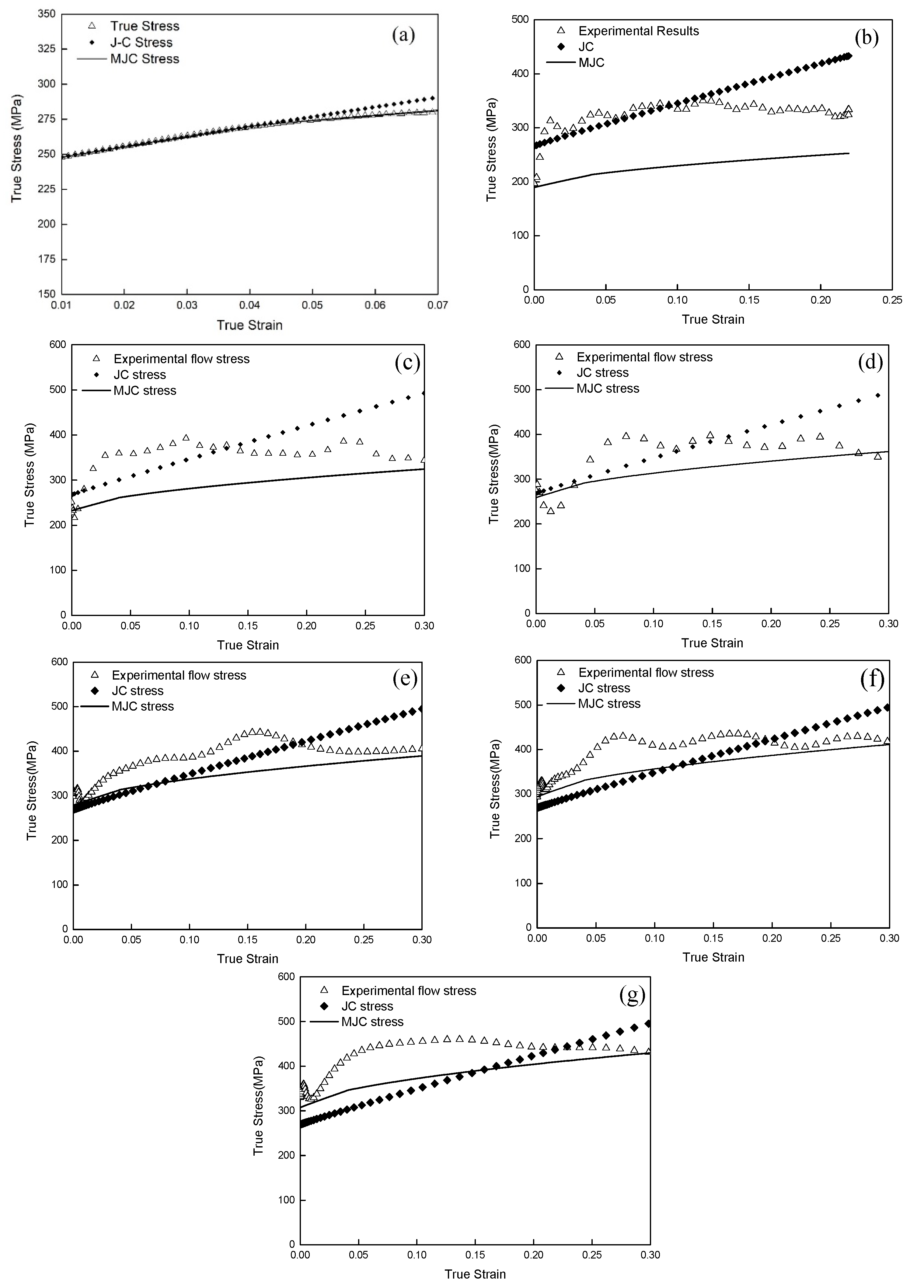
3.2. Analysis of Constitutive Model Accuracy

It can be seen from Section 3.1. that the modified J–C constitutive model considered the coupling effects of strain hardening effect, strain rate hardening effect, and thermal softening effect comparing by the basic J–C constitutive model. To analyze the accuracy of two constitutive models, the predicted flow stress, which is calculated by Equations (11) and (12), was compared with the experimental results.

As seen from Figure 7a–g, the stress–strain curve predicted by the modified J–C constitutive equation shows a consistent trend with the true stress–strain curve obtained by the experimental results. When the strain rate was less than 8000 s^‒1, the stress predicted by the J–C constitutive equation approached the true flow stress. The stress predicted by the modified J–C model was closer to the experimental flow stress at 8000 s^‒1. As the strain rate rose to 12,000 s^‒1, the predicted stress by the modified J–C constitutive model was obviously more accurate.

From the above, the J–C constitutive model can only predict flow stress at lower strain rates. The accuracy of the improved J–C constitutive equation increased gradually with the increase of the strain rate at the reference temperature. Especially at high strain rate conditions, the accuracy of the modified J–C constitutive equation was greatly improved compared with the J–C constitutive equation, which is closer to the experimental flow stress.

Figure 8 presents the comparison of the stresses calculated by the two constitutive models and flow stresses measured by SHPB experiments in different temperatures at 2000 s⁻¹. It is obvious that the predicted stress by the modified J–C constitutive equation was basically consistent with the experimental flow stress. But the error of stress predicted by the J–C equation increased gradually as the temperature rose. This implies that the J–C constitutive equation can only predict the flow stress at lower temperatures.

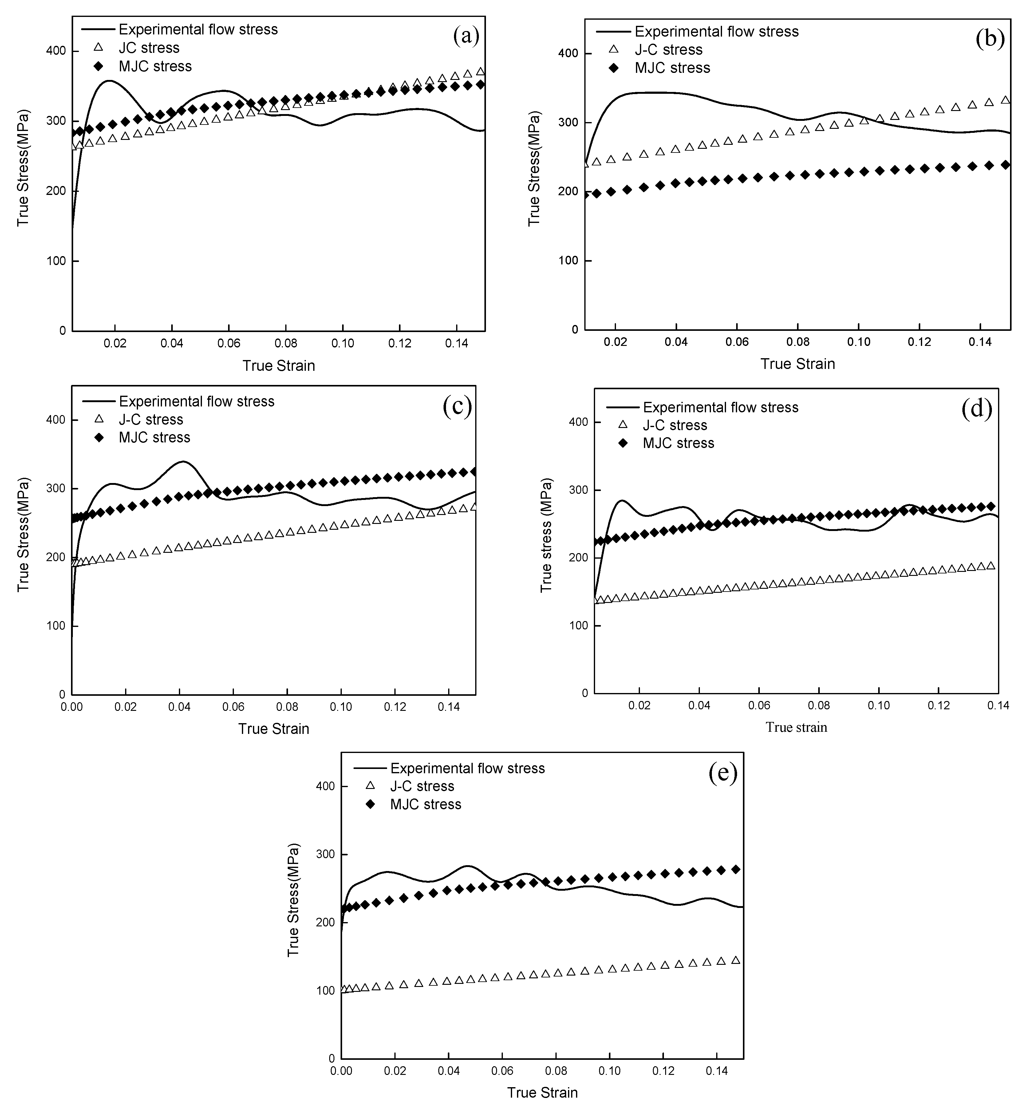
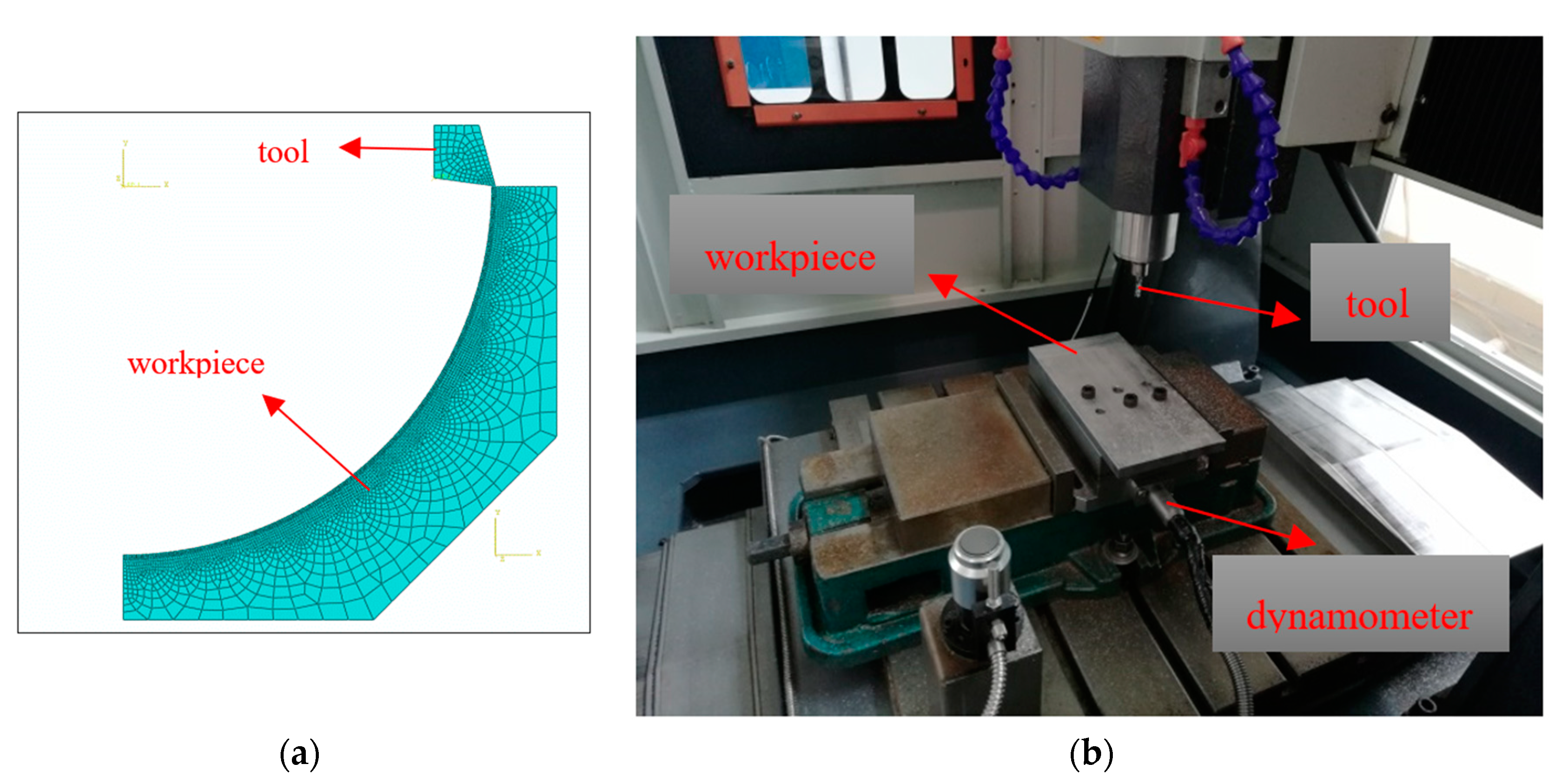
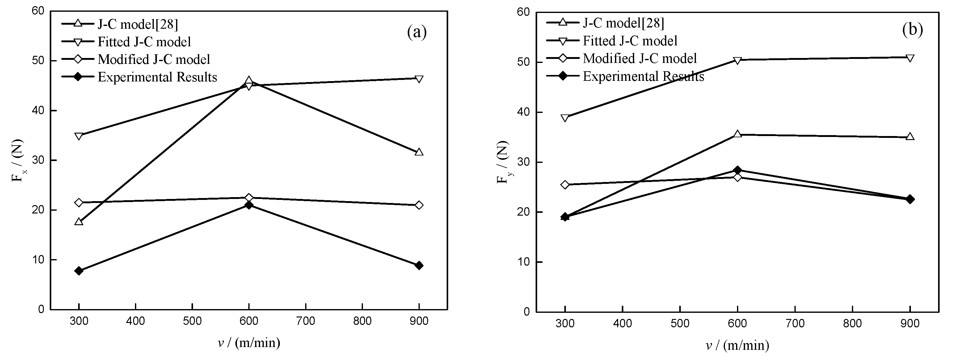
3.3. Model Validation

Considering the characteristics of milling, a two-dimensional cycloidal cutting simulation model was built based on the two J–C constitutive equations and the J–C model [28]. The milling experiments were performed with a four-edge carbide tool with diameters of 6 mm to validate the simulation results. In this study, numerical control engraving and milling machine SXDK6050D was used, with a spindle speed that could reach up to 100,000 r/min. A Kister dynamometer was used to measure the cutting forces in three directions during the milling process. The workpiece size was 200 × 100 × 10 mm³. The established two-dimensional finite element model and milling experimental setup are shown in Figure 9a,b.

Table 2. The parameters of milling experiments.

Cutting Speed v (m/min)	Spindle Speed n (r/min)	Feed Rate fz (mm/z)	Milling Width ae (mm)	Cutting Depth ap (mm)
300	15,924	0.025	3	0.5
600	31,847
900	47,770

presents the machining parameters of milling experiments.

Figure 10a,b illustrates the comparison between the feed force (Fx) and tangential force (Fy) simulated by different J–C constitutive models and the cutting force measured by experiments. It can be seen that the cutting force predicted by the improved J–C constitutive equation was closer to the cutting force measured experimentally compared with the other two J–C constitutive equations. In addition, Figure 10b illustrates that the cutting force simulated by the improved J–C constitutive model showed the same trend as that measured by the experiment. The cutting force first rose and then decreased with the cutting speed increasing, reaching a maximum at 600 m/min.

In summary, the improved J–C constitutive equation has higher accuracy. This is because the classical J–C constitutive equation assumes that the strain hardening effect, the strain rate hardening effect, and the thermal softening effect are independently affected [29,30,31]. This is not consistent with the actual situation. However, the improved J–C constitutive equation takes into account the independent effects and the coupling effect of strain strengthening effect, strain rate strengthening effect, and thermal softening effect on the flow stress. Since the improved J–C constitutive model can accurately predict the flow stress at high strain rate and high temperature, it is suitable for various metals and alloys and can describe the relationship between stress and strain, strain rate, and temperature during high-speed cutting of alloys.

4. Conclusions

This paper fitted two J–C constitutive models based on the true stress–strain curve in different strain rates and temperatures of ADC12 alloy. By comparing the simulated cutting force and experimental cutting force, the cycloidal cutting finite element model could be validated. The conclusions are as follows.

(1) The flow stress rose gradually when the strain rate increased from 1000 s^‒1 to 12,000 s^‒1 at 20 °C, but that decreased when the test temperature increased from 100 °C to 450 °C at 2000 s^‒1. By comparing the two constitutive models, it illustrated that the piecewise function can explain the strain effect on the flow stress more accurately, and the polynomial function can explain the strain rate and temperature effect on the flow stress more accurately;

(2) By contrasting the predicted flow stress and experimental results, it implies that the improved J–C constitutive model can predict the flow stress at high strain rates and high temperatures more accurately. The simulation cutting force by the improved J–C constitutive equation was verified by the high-speed milling experimental results.

References

1. Chen, D.H.; Jia, X.L.; Zhu, X.R. Research progress of cast aluminum alloy for engine cylinder head. Cast. Tech. 2010, 31, 882–887. [Google Scholar]
2. Yiran, H. Experimental Analysis and Cutting Stability Prediction of ADC12 Al-Si Alloy High Speed Milling; Dalian University of Technology: Dalian, China, 2014. [Google Scholar]
3. List, G.; Sutter, G.; Bouthiche, A. Cutting temperature prediction in high speed machining by numerical modelling of chip formation and its dependence with crater wear. Int. J. Mach. Tools Manuf. 2012, 54, 1–9. [Google Scholar] [CrossRef]
4. Cui, D.; Zhang, D.; Wu, B.; Luo, M. An investigation of tool temperature in end milling considering the flank wear effect. Int. J. Mech. Sci. 2017, 131, 613–624. [Google Scholar] [CrossRef]
5. Liang, X.; Liu, Z. Tool wear behaviors and corresponding machined surface topography during high-speed machining of Ti-6Al-4V with fine grain tools. Tribol. Int. 2018, 121, 321–332. [Google Scholar] [CrossRef]
6. Sugita, N.; Ishii, K.; Furusho, T.; Harada, K.; Mitsuishi, M. Cutting temperature measurement by a micro-sensor array integrated on the rake face of a cutting tool. CIRP Ann. Manuf. Technol. 2015, 64, 77–80. [Google Scholar] [CrossRef]
7. de-Buruaga, M.S.; Soler, D.; Aristimuño, P.X.; Esnaola, J.A.; Arrazola, P.J. Determining tool/chip temperatures from thermography measurements in metal cutting. Appl. Therm. Eng. 2018, 145, 305–314. [Google Scholar] [CrossRef]
8. Heigel, J.C.; Whitenton, E.; Lane, B.; Donmez, M.A.; Madhavan, V.; Kingsley, W.M. Infrared Measurement of the Temperature at the Tool-Chip Interface While Machining Ti-6Al-4V. J. Mater. Process. Technol. 2016, 243, 123–130. [Google Scholar] [CrossRef] [Green Version]
9. Xiong, Y.; Wang, W.; Jiang, R.; Kunyang, L. Analytical model of workpiece temperature in end milling in-situ TiB2/7050Al metal matrix composites. Int. J. Mech. Sci. 2018, 149, 258–297. [Google Scholar] [CrossRef]
10. Möhring, H.C.; Kushner, V.; Storchak, M.; Stehle, T. Temperature calculation in cutting zones. CIRP Annals 2018, 67, 61–64. [Google Scholar] [CrossRef]
11. Li, L.; Li, B.; Ehmann, K.F.; Li, X. A thermo-mechanical model of dry orthogonal cutting and its experimental validation through embedded micro-scale thin film thermocouple arrays in PCBN tooling. Int. J. Mach. Tools Manuf. 2013, 70, 70–87. [Google Scholar] [CrossRef]
12. Huang, K.; Yang, W. Analytical Model of Temperature Field in Workpiece Machined Surface Layer in Orthogonal Cutting. J. Mater. Process. Technol. 2015, 229, 375–389. [Google Scholar] [CrossRef]
13. Wu, B.; Cui, D.; He, X.; Zhang, D.; Tang, K. Cutting tool temperature prediction method using analytical model for end milling. Chin. J. Aeronaut. 2016, 29, 1788–1794. [Google Scholar]
14. Karaguzel, U.; Bakkal, M.; Budak, E. Modeling and Measurement of Cutting Temperatures in Milling. Procedia CIRP 2016, 46, 173–176. [Google Scholar] [CrossRef] [Green Version]
15. Zhou, F.; Wang, X.; Hu, Y.; Ling, L. Modeling temperature of non-equidistant primary shear zone in metal cutting. Int. J. Therm. Sci. 2013, 73, 38–45. [Google Scholar] [CrossRef]
16. Özel, T.; Altan, T. Determination of workpiece flow stress and friction at the chip-tool contact for high-speed cutting. Int. J. Mach. Tools Manuf. 2000, 40, 133–152. [Google Scholar] [CrossRef]
17. Xu, D.; Feng, P.; Li, W.; Ma, Y. An improved material constitutive model for simulation of high-speed cutting of 6061-T6 aluminum alloy with high accuracy. Int. J. Adv. Manuf. Technol. 2015, 79, 1043–1053. [Google Scholar] [CrossRef]
18. Johnson, G.R.; Cook, W. A Constitutive Model and Data for Metals Subjected to Large Strain, High Strain Rate and High Temperature. In Proceedings of the 15th International Symposium on Ballistics, The Hague, The Netherlands, 19–21 April 1983. [Google Scholar]
19. Shi, J.; Liu, C.R. The influence of material models on finite element simulation of machining. J. Manuf. Sci. Eng. Trans. ASME 2004, 126, 849–857. [Google Scholar] [CrossRef]
20. Liang, R.; Khan, A.S. A critical review of experimental results and constitutive models for BCC and FCC metals over a wide range of strain rates and temperatures. Int. J. Plast. 1999, 15, 963–980. [Google Scholar] [CrossRef]
21. Kolsky, H. An Investigation of the Mechanical Properties of Materials at very High Rates of Loading. Proc. Phys. Soc. Sect. B 1949, 62, 676–700. [Google Scholar] [CrossRef]
22. Umbrello, D.; M’Saoubi, R.; Outeiro, J.C. The influence of Johnson—Cook material constants on finite element simulation of machining of AISI 316L steel. Int. J. Mach. Tools Manuf. 2007, 47, 462–470. [Google Scholar] [CrossRef]
23. Hua, Y.-Z.; Guan, L.-W.; Liu, X.-J.; Cui, H.-L. Research and revise on constitutive equation of 7050-T7451 aluminum alloy in high strain rate and high temperature condition. J. Mater. Eng. 2012, 2, 7–13. [Google Scholar]
24. Rasaee, S.; Mirzaei, A.H. Constitutive Modeling of 2024 Aluminum Alloy Based on the Johnson–Cook Model. Trans. Indian Inst. Metals 2019, 72, 1023–1030. [Google Scholar] [CrossRef]
25. Guo, Y.B. An integral method to determine the mechanical behavior of materials in metal cutting. J. Mater. Process. Technol. 2003, 142, 72–81. [Google Scholar] [CrossRef]
26. Sima, M.; Özel, T. Modified material constitutive models for serrated chip formation simulations and experimental validation in machining of titanium alloy Ti–6Al–4V. Int. J. Mach. Tools Manuf. 2010, 50, 943–960. [Google Scholar] [CrossRef]
27. Karaguzel, U.; Budak, E. Investigating effects of milling conditions on cutting temperatures through analytical and experimental methods. J. Materi. Process. Technol. 2018, 262, 532–540. [Google Scholar] [CrossRef]
28. Bi, J.; Cong, M.; Liu, D.; Xu, X. Simulation and experimental analysis of ADC12 Al-Si alloy cutting. Combination Mach. Tools Autom. Process. Technol. 2017, 1, 127–130. (In Chinese) [Google Scholar]
29. Bani, A.A.; Hanzaki, A.Z.; Pishbin, M.H.; Haghdadi, N. A comparative study on the capability of Johnson–Cook and Arrhenius-type constitutive equations to describe the flow behavior of Mg–6Al–1Zn alloy. Mech. Mater. 2014, 71, 52–61. [Google Scholar] [CrossRef]
30. Lin, Y.C.; Li, L.-T.; Fu, Y.-X.; Jiang, Y.-Q. Hot compressive deformation behavior of 7075 Al alloy under elevated temperature. J. Mater. Sci. 2012, 47, 1306–1318. [Google Scholar] [CrossRef]
31. Lin, Y.C.; Li, Q.-F.; Xia, Y.-C.; Li, L.-T. A phenomenological constitutive model for high temperature flow stress prediction of Al–Cu–Mg alloy. Mater. Sci. Eng. A 2012, 534, 654–662. [Google Scholar] [CrossRef]
Figure 1. Diagram of quasi-static experimental equipment.
Metals 10 01038 g001
Figure 2. Device diagram of split Hopkinson pressure bar experiment.
Metals 10 01038 g002
Figure 3. The true stress–strain curve of ADC12 aluminum alloy in the (a) quasi-static experiment; (b) different strain rates at 20 °C; and (c) different temperatures at 2000 s‒1.
Metals 10 01038 g003
Figure 4. The fit line of the relation between ln ( σ ¯ A ) and ln ( ε ¯ P ) by the (a) J–C model and the (b) Modified J–C model at ε ˙ P =0.0003 s‒1 and T = 20 °C.
Metals 10 01038 g004
Figure 5. The relation between ln ε ˙ * and σ ¯ / ( A + B ε ¯ P n ) at the reference temperature.
Metals 10 01038 g005
Figure 6. (a) The relation between ln ( T ) and ln ( 1 σ / ( A + B ε ¯ 0 P n ) ) at 2000 s‒1. (b) The relation between K T and T at 2000 s‒1.
Metals 10 01038 g006
Figure 7. Comparison between experimental and predicted stresses at (a) reference strain rate; (b) 2000 s‒1; (c) 4000 s‒1; (d) 6000 s‒1; (e) 8000 s‒1; (f) 10,000 s‒1; (g) 12,000 s‒1.
Metals 10 01038 g007
Figure 8. Comparison between experimental and predicted stress at (a) 100 °C; (b) 200 °C; (c) 300 °C; (d) 400 °C; (e) 450 °C.
Metals 10 01038 g008
Figure 9. (a) Cycloid finite element model; (b) experimental setup of high-speed milling.
Metals 10 01038 g009
Figure 10. Diagram of cutting force changing with speed: ((a) Feed direction force Fx, (b) tangential force Fy).
Metals 10 01038 g010