Changes of Multiphase Flow Patterns during Steel Tapping with Simultaneous Argon Bottom Stirring in the Ladle

 , ,
, , 
Abstract
:1. Introduction
2. The Mathematical Model
2.1. Model Assumptions
- The system is considered isothermal and then, there is no need to solve the equation for energy transport. The temperature of the system is 1620 °C. Argon stirring proved to be effective to decrease large temperature gradients of liquid steel existing after a relatively long stand still time of the ladle, in just only three seconds [7,8] of stirring. Therefore, with the combined effect of the impinging jet and the argon stirring, the temperature gradients are negligible.
- The previous assumption involves, implicitly, that the buoyancy forces are negligible compared with the inertial forces. The validity of this assumption is based on the work of Berg et al. [4] who previously simulated the flow patterns under non-isothermal and non-isothermal conditions without finding any signifying differences of the flow patterns of steel.
- The physical properties of the steel, argon and air were evaluated at the film temperature (average between room and liquid steel temperatures).
- As a first approach to deal with this complex flow, the effects of additions such as ferro-alloys and fluxes on the flow patterns are not considered. Therefore, only the gaseous and liquid phases are involved in these simulations.
- According to Iron thermodynamics [9] the solubility of air and argon in liquid steel is negligible implying that there is not mass transfer among the phases.
- The impinging jet of steel has a compact structure. This assumption is reasonable if the EBT system is clean of debris, this is true specifically when the sleeve is new.
- Strictly speaking, air and argon form a gaseous phase. However, since the densities are different, in this work both gases are considered as different phases by using a jumping boundary condition at the argon-air interphases. This trick will allow for tracking the segregation of argon inside and outside the bath.
2.2. Dynamics of the Multiphase Flow
2.3. Boundary Conditions
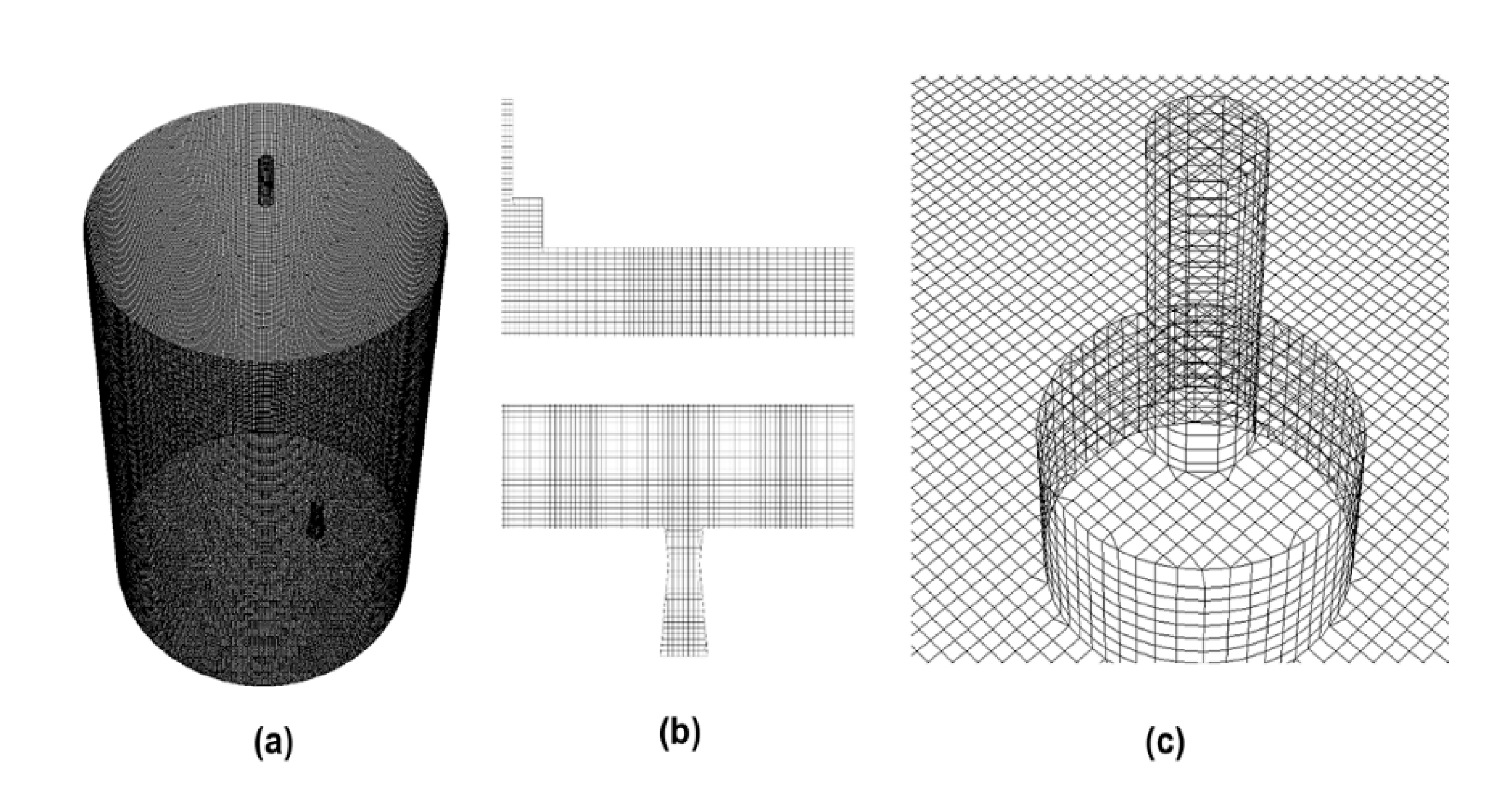
2.4. Method of Solution
3. Results and Discussion
4. Conclusions
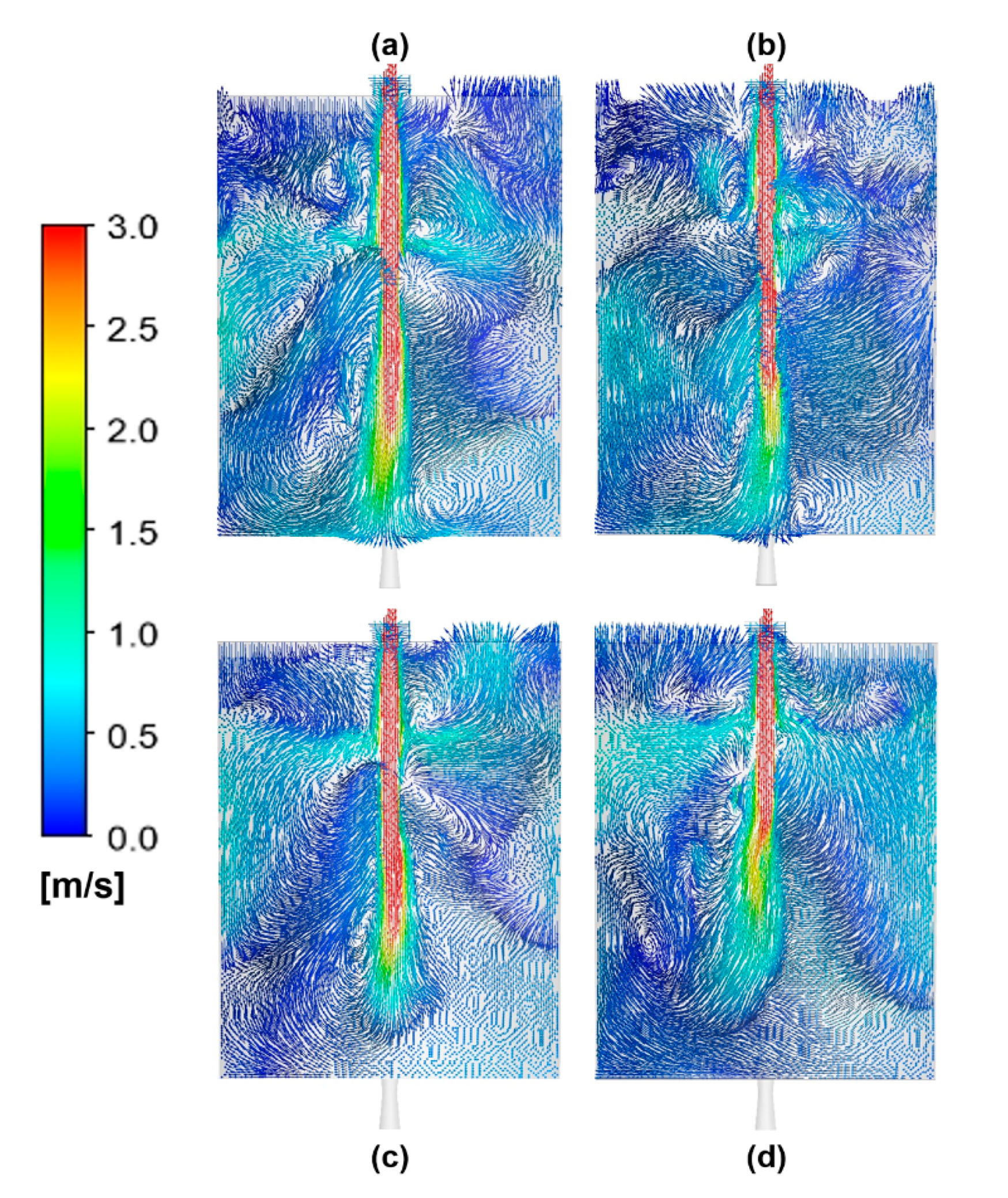
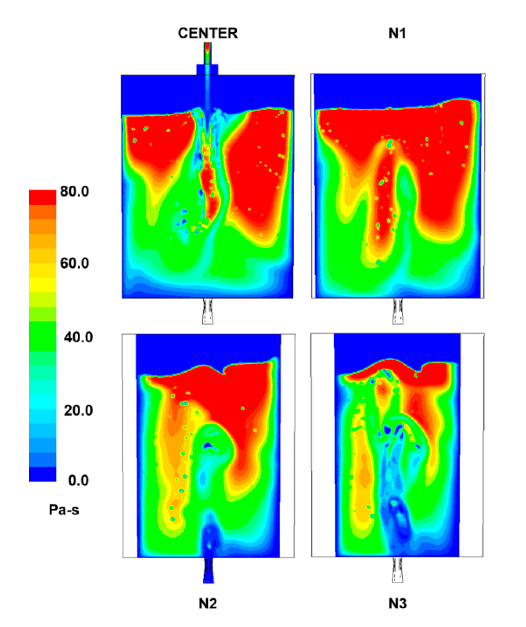
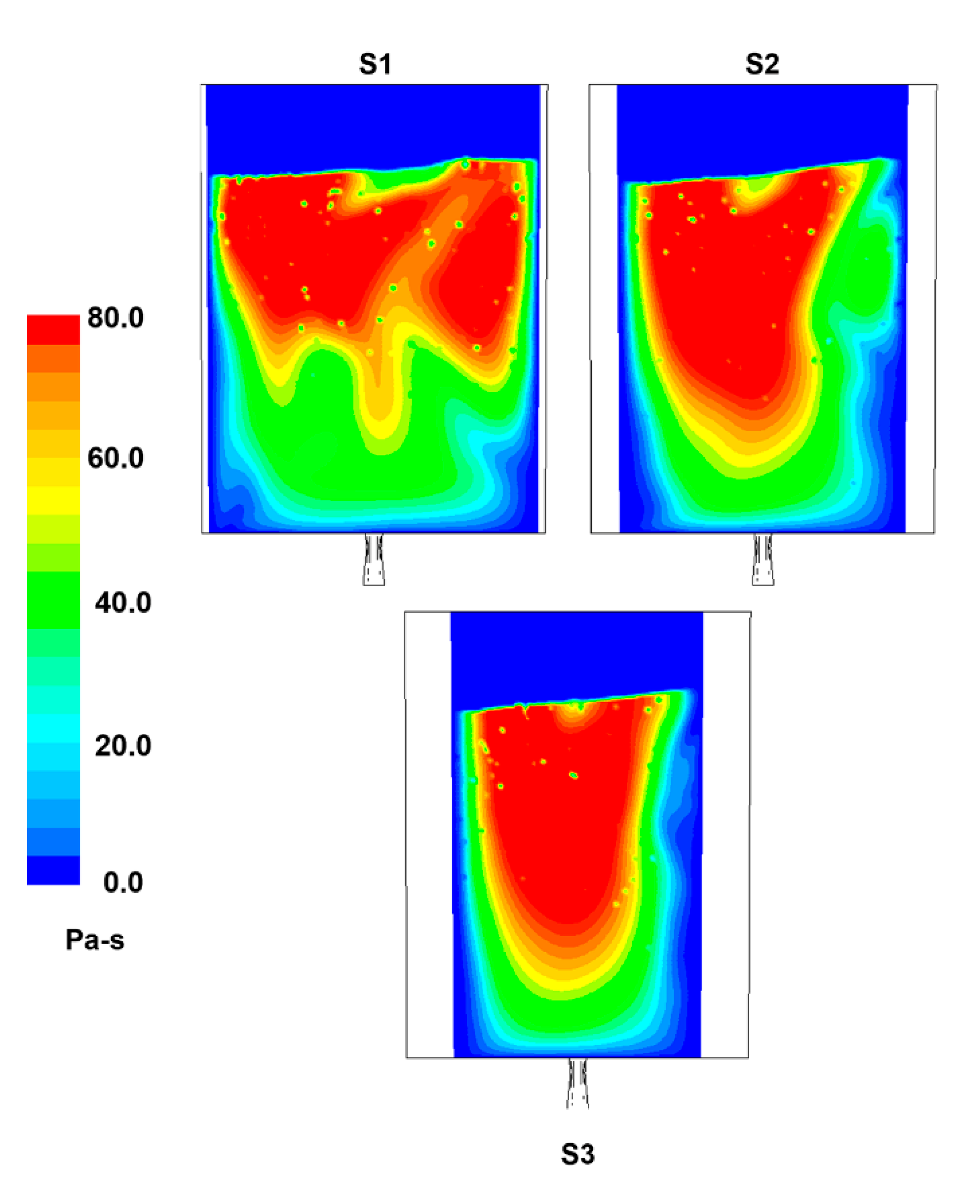
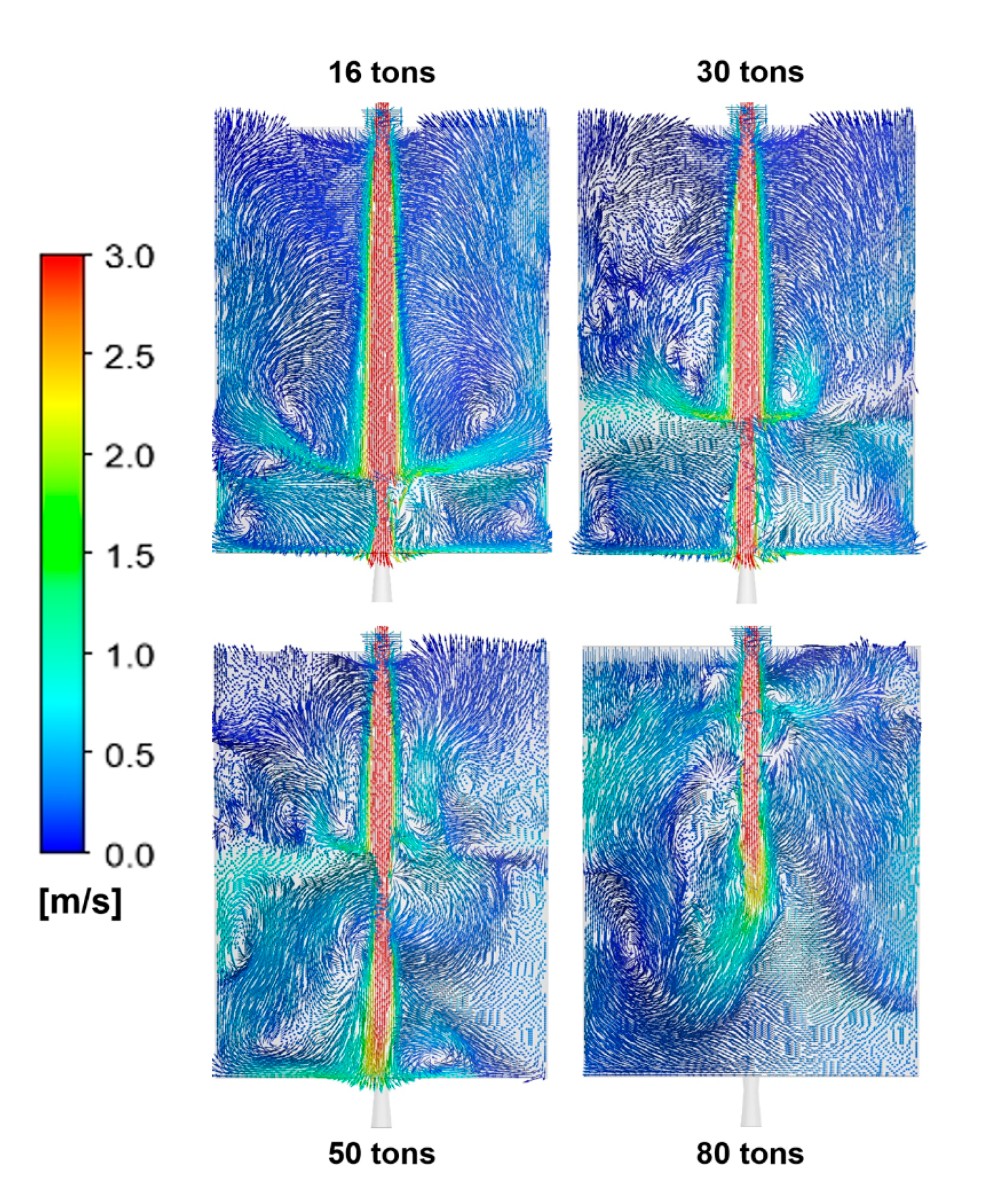
- At low liquid steel levels in the ladle, the flow turbulence is smaller than at high steel levels. A tall bath allows larger recirculations of the flow, enhancing the transport of kinetic energy, enhancing the turbulence of the system.
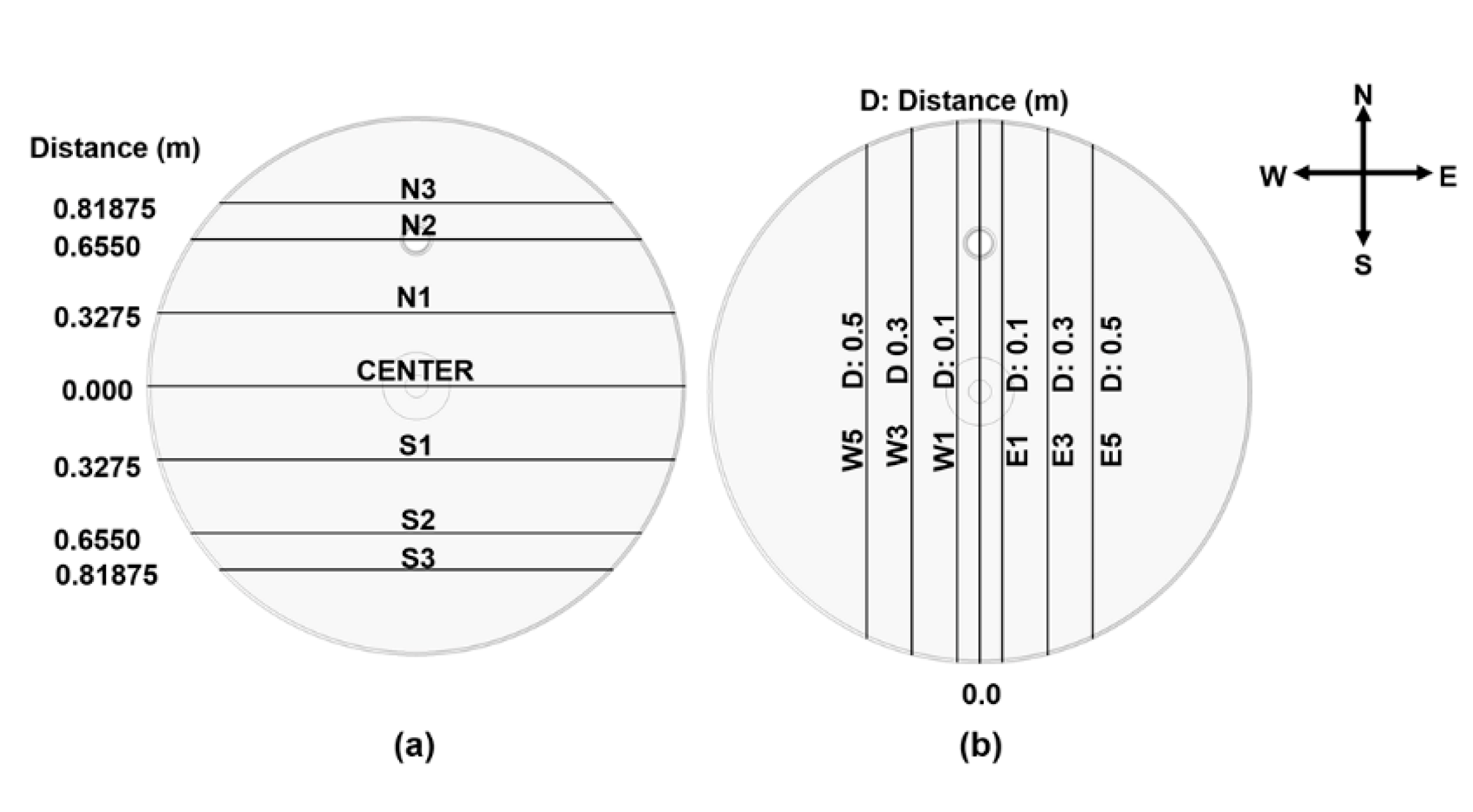
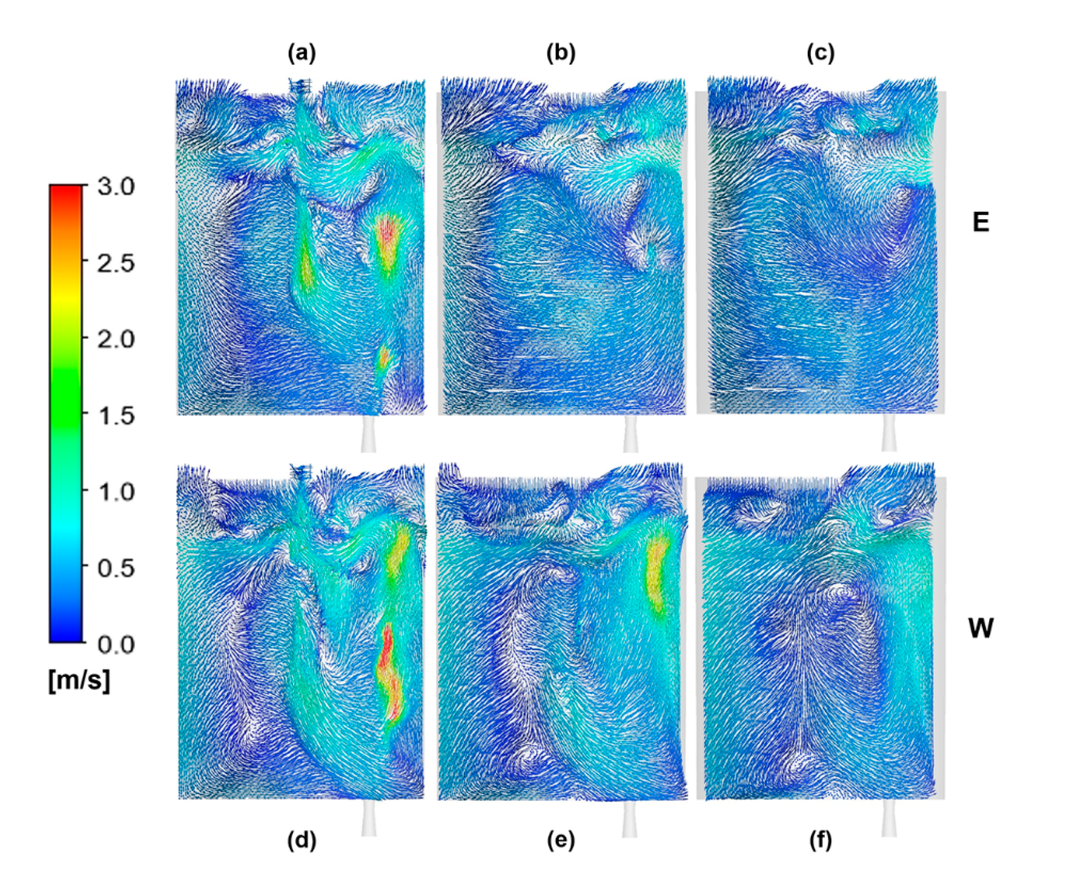
- The eccentric position of the argon plug in the ladle bottom and the impinging jet interact in such a way that the melt streams formed after impacting the ladle bottom bend the argon plume inducing asymmetric flows throughout all the liquid volume at any bath level.
- The bending effect of the imping jet and the resultant deviation of the argon plume remain during the full time of the ladle filling operation. Besides the unsteadiness of the velocity fields of this complex flow is a clear indication of the existing potential for particle melting and thermal and chemical mixing during steel tapping.
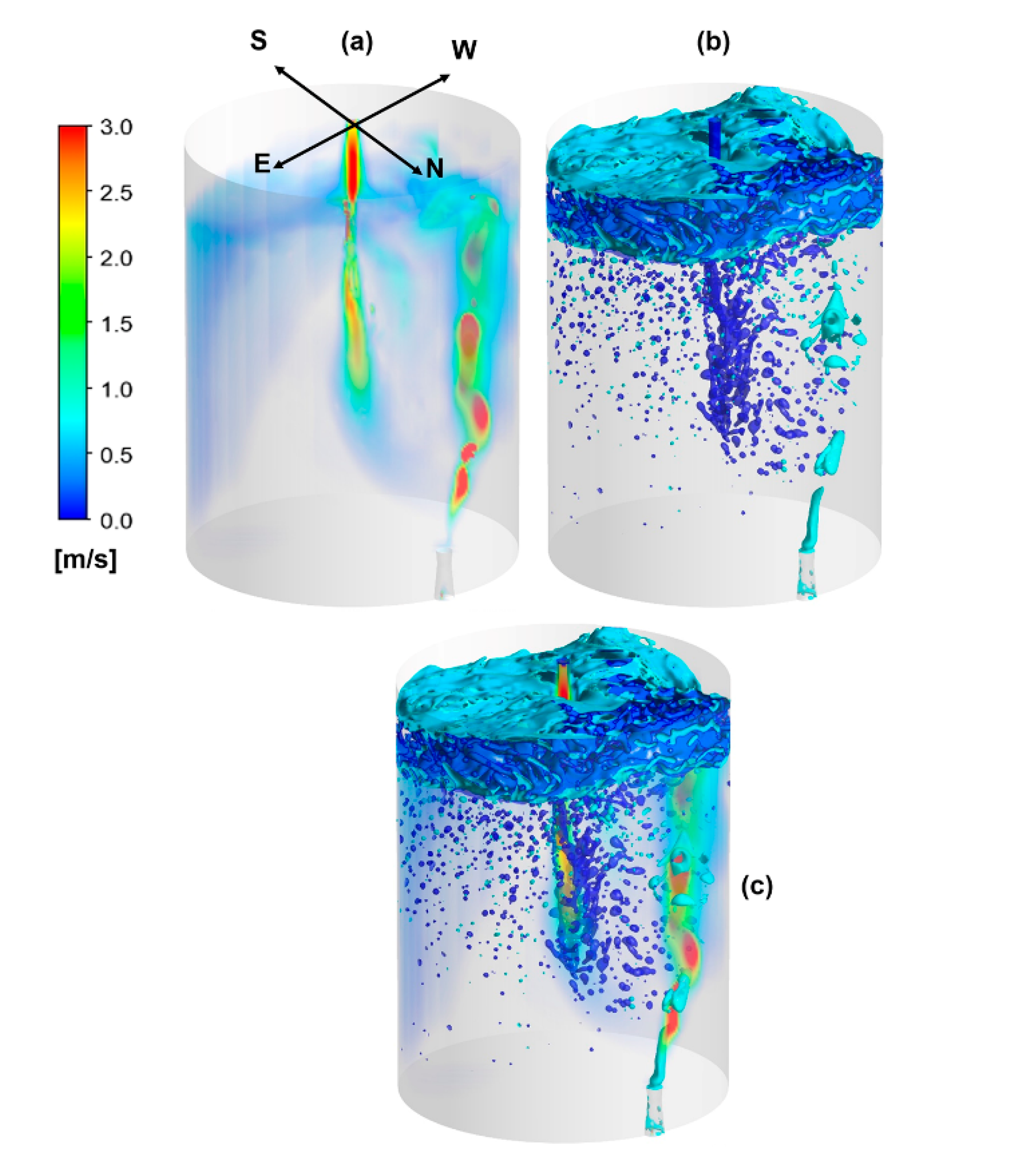
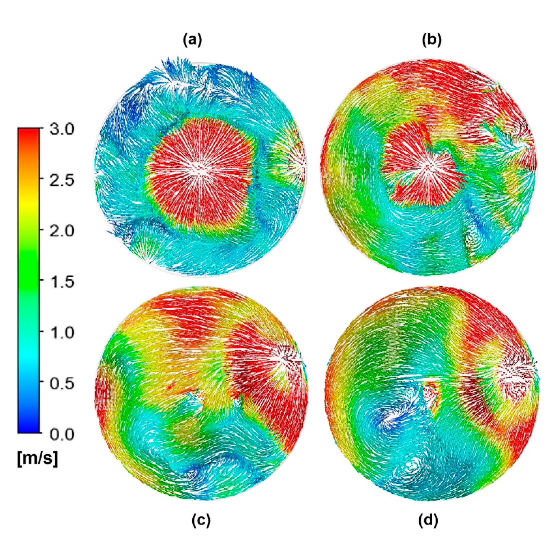
- The argon bubbles travel all the plume height in the plume and when it reaches the bath surface, this gas is dragged to the opposite side to where the plug is located forming a thick blanket of this gas covering a superficial mixture of steel and air. Due to the higher density of argon than air, it is concluded that this blanket decreases the direct contact between air and steel during the ladle filling operation.
- Part of the argon, forming the blanket, is dragged inside the bath bulk by the impinging jet. These results encourage further simulations aimed at the optimization of the steel tapping operation, which is not a trivial issue.
Author Contributions
Funding
Acknowledgments
Conflicts of Interest
Nomenclature
| Cμ | Constant in the turbulence model |
| H | radius of curvature |
| I k | Identity matrix |
| k | kinetic energy |
| t | time |
| u | velocity |
| V | Volume |
| α | volume fraction |
| ε | dissipation rate of kinetic energy |
| μ | viscosity |
| ρ | density |
| σ | surface tension |
| T | strain stress |
| Χ | phase indicator |
| q | phase |
| m | mixture |
| n | normal |
| I | interface |
References
- Guthrie, R.I.L.; Clift, R.; Henein, H. Contacting problems associated with aluminum and ferro-alloy additions in steelmaking-hydrodynamic aspects. Met. Mater. Trans. B 1975, 6, 321–329. [Google Scholar] [CrossRef]
- Tanaka, M.; Mazumdar, D.; Guthrie, R.I.L. Motions of alloying additions during furnace tapping in steelmaking processing operations. Met. Mater. Trans. B 1993, 24, 639–648. [Google Scholar] [CrossRef]
- Rodríguez-Ávila, J.; Morales, R.D.; Nájera-Bastida, A. Numerical Study of multiphase Flow dynamics of plugging jets in liquid steel and trajectories of ferroalloy additions in a ladle during tapping operations. ISIJ Int. 2012, 52, 814–822. [Google Scholar] [CrossRef]
- Berg, H.; Laux, H.; Johansen, S.T. Flow pattern and alloy dissolution during tapping of steel furnaces. Ironmak. Steelmak. 1999, 26, 127–139. [Google Scholar] [CrossRef]
- Milanovic, I.; Hammad, K.J. PIV Study of the Near-Field Region of a Turbulent Round Jet. In Proceedings of the ASME 2010 3rd Joint US-European Fluids Engineersing Summer Meeting and 8th International Conference on Nanochannels, Microchannels and Minichannels, Montreal, QC, Canada, 1–5 August 2010. [Google Scholar]
- Iguchi, M.; Okita, K.; Yamamoto, F. Workshop on multicomponent and multiphase flow dynamics. Int. J. Multiph. Flows 1998, 24, 523–537. [Google Scholar] [CrossRef]
- Dávila, O.; García-Demedices, L.; Morales, R.D. Mathematical simulation of fluid dynamics during steel draining operations from a ladle. Met. Mater. Trans. B 2006, 37, 71–87. [Google Scholar] [CrossRef]
- Grip, C.E.; Jonsson, L.; Jonsson, P.; Jonsson, K.O. Numerical prediction and experimental verification of thermal stratification during holding in pilot plant and production ladles. ISIJ Int. 1999, 39, 715–721. [Google Scholar] [CrossRef]
- Darken, L.S.; Gurry, R.W.; Bever, M.B. Physical Chemistry of Metals; McGraw-Hill Books: New York, NY, USA, 1953; pp. 372–395. [Google Scholar]
- Jakobsen, H.A. Chemical Reactor Modelling; Springer: New York, NY, USA, 2014; pp. 300–389. [Google Scholar]
- Yeoh, G.H. Computational Techniques for Multiphase-Flows; Butterworth-Heinemann: Oxford, UK, 2010; pp. 215–232. [Google Scholar]
- Wilcox, D.C. Turbulence Modeling for CFD; DCW Industries: La Cañada, CA, USA, 2000; pp. 103–104. [Google Scholar]
- Tennekes, H.; Lumley, J.L. A First Course in Turbulence; MIT Press Journals: Cambridge, MA, USA, 1972; pp. 27–30. [Google Scholar]
- Ferziger, J.H.; Peric, M. Computational Methods for Fluid Dynamics; Springer: New York, NY, USA, 2002; pp. 72–74. [Google Scholar]
- ANSYS, Inc. Available online: www.ansys.com (accessed on 10 April 2019).
- Youngs, D.L. Numerical Methods for Fluid Dynamics; Morton, K.W., Baines, M.J., Eds.; Academic Press: London, UK, 1982; pp. 273–385. [Google Scholar]
- Chung, T.J. Computational Fluid Dynamics; Cambridge University Press: London, UK, 2002; pp. 218–220. [Google Scholar]
- Bird, R.B.; Stewart, W.E.; Lightfoot, E.N. Transport Phenomena; Wiley International: Hoboken, NJ, USA, 1960; p. 153. [Google Scholar]
- Issa, R.I. Solution of the implicitly discretized fluid flow equations by operator-splitting. Comp. Phys. 1986, 62, 40–65. [Google Scholar] [CrossRef]
- Morales, R.D.; Calderón-Hurtado, F.A.; Chattopadhyay, K.; Guarneros, S.J.G. Physical and Mathematical Modeling of Flow Structures of Liquid Steel in Ladle Stirring Operations. Met. Mater. Trans. A 2020, 51, 628–648. [Google Scholar] [CrossRef]


| Phase | Density | Viscosity |
|---|---|---|
| Liquid Steel | 7100 | 0.006 |
| Argon | 0.458 | 5.7 × 10⁻⁵ |
| Air | 0.3289 | 4.36 × 10⁻⁵ |
| Item | Description | Observations |
|---|---|---|
| Electric Arc Furnace | AC EAF with a capacity of 100 tons, hot heel of 12–15 tons | Burners, oxygen lances and EBT system |
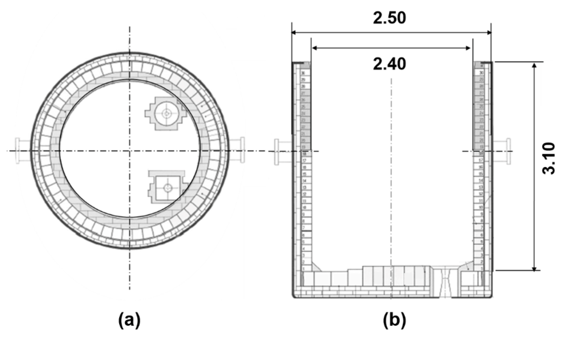
| Ladle | Capacity of 80 tons, straight geometry, dolomite lining | Eccentric argon plug, pneumatic stirring |
| EBT | Sleeve diameter is 114 mm, flow rate of argon is 400 L/min | Straight sleeve pointing toward the center of the ladle |
| EBT-Ladle bottom | The distance between the tip of the EBT sleeve and the ladle bottom is 3.50 m | The length of the EBT is 0.90 m, embedded in the bottom of the EAF |
| Steel throughput | Between 16 and 23 tons/min, a magnitude of 20 ton/min was assumed | The steel throughput depends on the wear condition of the sleeve |
© 2020 by the authors. Licensee MDPI, Basel, Switzerland. This article is an open access article distributed under the terms and conditions of the Creative Commons Attribution (CC BY) license (http://creativecommons.org/licenses/by/4.0/).
Share and Cite
Nájera-Bastida, A.; Rodríguez-Ávila, J.; Guarneros-Guarneros, J.; Morales, R.D.; Chattopadhyay, K. Changes of Multiphase Flow Patterns during Steel Tapping with Simultaneous Argon Bottom Stirring in the Ladle. Metals 2020, 10, 1036. https://doi.org/10.3390/met10081036
Nájera-Bastida A, Rodríguez-Ávila J, Guarneros-Guarneros J, Morales RD, Chattopadhyay K. Changes of Multiphase Flow Patterns during Steel Tapping with Simultaneous Argon Bottom Stirring in the Ladle. Metals. 2020; 10(8):1036. https://doi.org/10.3390/met10081036
Chicago/Turabian StyleNájera-Bastida, Alfonso, Jafeth Rodríguez-Ávila, Javier Guarneros-Guarneros, Rodolfo D. Morales, and Kinnor Chattopadhyay. 2020. "Changes of Multiphase Flow Patterns during Steel Tapping with Simultaneous Argon Bottom Stirring in the Ladle" Metals 10, no. 8: 1036. https://doi.org/10.3390/met10081036
APA StyleNájera-Bastida, A., Rodríguez-Ávila, J., Guarneros-Guarneros, J., Morales, R. D., & Chattopadhyay, K. (2020). Changes of Multiphase Flow Patterns during Steel Tapping with Simultaneous Argon Bottom Stirring in the Ladle. Metals, 10(8), 1036. https://doi.org/10.3390/met10081036