Comparison of Bayesian Methods on Parameter Identification for a Viscoplastic Model with Damage

Abstract

The state of materials and accordingly the properties of structures are changing over the period of use, which may influence the reliability and quality of the structure during its life-time. Therefore, identification of the model parameters of the system is a topic which has attracted attention in the content of structural health monitoring. The parameters of a constitutive model are usually identified by minimization of the difference between model response and experimental data. However, the measurement errors and differences in the specimens lead to deviations in the determined parameters. In this article, the focus is on the identification of material parameters of a viscoplastic damaging material using a stochastic simulation technique to generate artificial data which exhibit the same stochastic behavior as experimental data. It is proposed to use Bayesian inverse methods for parameter identification and therefore the model and damage parameters are identified by applying the Transitional Markov Chain Monte Carlo Method (TMCMC) and Gauss-Markov-Kalman filter (GMKF) approach. Identified parameters by using these two Bayesian approaches are compared with the true parameters in the simulation and with each other, and the efficiency of the identification methods is discussed. The aim of this study is to observe which one of the mentioned methods is more suitable and efficient to identify the model and damage parameters of a material model, as a highly non-linear model, using a limited surface displacement measurement vector and see how much information is indeed needed to estimate the parameters accurately.

1. Introduction

In order to predict the behavior of mechanically loaded metallic materials, constitutive models are applied, which present a mathematical frame for the description of elastic and inelastic deformation. All inelastic constitutive models contain parameters which have to be identified for a given material from experiments [1].

There are few investigations on the simplest material model, the elasticity model, to identify only very few parameters of the model where sampling approaches like the Metropolis algorithm and its modifications are employed. Pacheco et al. [2] investigated a three-point bending test to identify elastic behavior and calibration is done by solving the inverse problem in a Bayesian setting by using the Metropolis-Hastings algorithm. Only elastic moduli are identified without considering the error. Slonski et al. [3] also applied a sequential particle filter on an elastic model and Young’s modulus was estimated, where the Bayesian setting was compared to the deterministic approach, and the Bayesian setting was preferred. The elastic modulus of a polymeric material is updated by Zhang et al. [4], where a Markov Chain Monte Carlo method is used, but very high computation time is reported. Further, Young’s modulus is estimated for a considered material by Gallina et al. [5] by applying a multi dimensional Markov Chain Monte Carlo method. A similar Bayesian approach for composite materials to estimate Young’s modulus is carried out by Pieczonka et al. [6]. Arnst et al. [7] have applied a Markov Chain Monte Carlo method by using polynomial chaos expansion to identify Young’s modulus of an elastic model.

Only few investigations were carried out on enriched material models such as a viscoelastic model to identify the few parameters by employing the Metropolis-Hastings technique and the classical Markov Chain Monte Carlo method. Rappel et al. [8] studied an elastic and a viscoelastic model where the measurement error is considered. Bayesian inference is applied to estimate only the elasticity modulus by applying an adaptive Metropolis-Hastings technique. An et al. [9] investigated a crack model by a classical Markov Chain Monte Carlo method in order to estimate the parameters of a model which represent the size and position of the crack in the Bayesian setting. Also Hernandez et al. [10] applied a Markov Chain Monte Carlo method on a viscoelastic model in order to update its model parameters in a Bayesian setting, but the posterior distributions of the parameters are not updated properly. In fact, the parameters are not identified properly. Mahnken [11] has also applied a Markov Chain Monte Carlo method to estimate few parameters of a plasticity model. The damage parameters of a truss structure under model uncertainties are studied by Zheng et al. [12], where a multi-level Markov Chain Monte Carlo method is applied and the true values are not well estimated. Further, this approach suffers from high computation time. Another damage detection approach is applied by Nichols et al. [13] by applying a modified version of the Markov Chain Monte Carlo method.

There are other investigations in the Bayesian setting using the Markov Chain Monte Carlo method, and Madireddy et al [14], Wang and Zabaras [15], and Oh et al. [16] have carried out investigations on the identification of a material model by using its modified method. In studies carried out by Alvin [17], Marwala and Sibusiso [18], Daghia et al. [19], Abhinav and Manohar [20], Gogu et al. [21,22], and Koutsourelakis [23,24], the elastic parameters of the model are estimated stochastically. Fitzenz et al. [25], Most [26], and Sarkar et al. [27] investigated elastoplastic materials and thermodynamical material models to identify their model parameters. Other studies on viscoelastic models are carried out by Zhang et al. [28], Mehrez et al. [29], and Miles et al. [30]. Further investigations on viscoelastic models to estimate a higher number of model parameters are studied by Zhao and Pelegri [31], and by Kenz et al. [32]. The estimation of fatigue parameters using Markov Chain Monte Carlo methods is also studied by An et al. [33].

Few investigations in which the Kalman filter and its modifications are employed to identify the material model parameters can be found in literature. Hoshi et al. [34] have estimated the Young’s Modulus and Poisson’s ratio parameters of an organ model by an extended version of Kalman filter. The same study on an elastic model is carried out to identify the elastic constants of anisotropic materials using Kalman filter by Furukawa et al. [35]. Conte et al. [36] applied some modifications of Kalman filter on a nonlinear structural model to identify its parameters. Hendriks [37] investigated the possibility of identification of few parameters on a viscoelastic model representing the behavior of solid materials by using Kalman filter. Few parameters to identify on the crack path is carried out by Bolzon et al. [38] by employing Kalman filter. Nguyen et al. and Mahmoudi et al. [39,40,41] applied an extended Kalman filter on an elastoplastic model to identify the model parameters. Wall [42] and Nakamura et al. [43] also applied a modification of Kalman filter on a viscoplastic model to determine its model parameters probabilistically. Further, Agmell et al. [44] have determined the Johnson–Cook constitutive model constants for an orthogonal cutting process by using the Kalman filter. Sevieri et al. [45,46,47] investigated the parameter identification of structural models in the framework of structural health monitoring. Marsili et al. [48,49,50,51,52] investigated the update the finite element model using functional approximation of the system response.

Elastic–plastic graded materials are observed by Bocciarelli et al. [53] and Gu et al. [54] in order to identify their model parameters by employing Kalman filter. The parameters of an elastic-damage interface model are also identified by Corigliano et al. [55,56] where the extended Kalman filter method is applied. Further, Ebrahimian et al. and Hariri-Ardebili et al. [57,58,59,60,61,62] investigated the damage parameter identification in the framework of structural health monitoring by using an extended version of Kalman filter. Damage detection for the purpose of health monitoring is also done by Yan et al. [63] by using the Kalman filter and other stochastic approaches by Kourehli et al. and Gharehbaghi et al. [64,65,66].

Although these discussed research for the identification of mechanical material models has been carried out, most of these previous research did not identify many parameters, e.g., hardening and damage parameters of the complex mechanical material models, did not quantify mostly the modeling uncertainties, did not properly deal with the ill-conditioning inherent based on the available data, and the methods employed have a high computation time even for the simplest material model considering a very few uncertain parameters. However, the uncertainty associated with the material model predictions can have a significant impact on the decision-making process in design, control, and health monitoring process.

In this paper, a viscoplastic model of Chaboche with damage is studied. The model contains five material parameters and three damage parameters which have to be determined from experimental data by using two Bayesian approaches, i.e., Transitional Markov Chain Monte Carlo method [67,68] and Gauss-Markov-Kalman filter approach [69,70,71,72]. The results of these two methods are compared and different aspects of them are evaluated. It should be noted that virtual data is employed instead of real experimental data. In addition, a cyclic tension-compression test is applied in order to extract the virtual data. A cyclic test is employed since the hardening equations as well as the damage equation could get involved so that the information from these equations can be observed.

Section 3 and Section 4 explain how to propagate the uncertainty in the model. The probabilistic model is reformulated from the deterministic model, and once the forward model is provided, the model parameters are updated using two mentioned stochastic approaches.

In Section 5 the desired parameters are identified from the measured data and the efficiency of methods is studied. In fact, the parameters which have been considered as uncertain parameters are updated and their uncertainties are narrowed using Bayesian techniques. The results are thoroughly studied and the identified parameters as well as the corresponding model responses are analyzed. Finally the prediction of the models is then compared with the measured data.

2. Model Problem

For viscoplasticity, the dissipation potential is given by

$${\varphi }_{vp}\left(\tilde{\mathit{\sigma }}\right)=\frac{k}{n+1}{〈\frac{{\tilde{\sigma }}_{ex}}{k}〉}^{n+1}\mathrm{with}{\tilde{\sigma }}_{ex}={\tilde{\sigma }}_{eq}-{\sigma }_y-R\mathrm{and}\langle ·\rangle =max(0,x)$$

(1)

in terms of the effective equivalent stress ${\tilde{\sigma }}_{eq}$ and the isotropic hardening R as time-varying variables. On the contrary, the yield stress ${\sigma }_y$, as well as k and n are further model parameters constant in time.

Based on the von-Mises yield-criterion the effective equivalent stress

$${\tilde{\sigma }}_{eq}=\sqrt{3I_2{\left(\tilde{\mathit{\sigma }}-\mathit{\chi }\right)}^d+\overline{D}{\left(I_1\left(\tilde{\mathit{\sigma }}-\mathit{\chi }\right)\right)}^2}$$

(2)

is described by the second Invariant

$$I_2{\left(\tilde{\mathit{\sigma }}-\mathit{\chi }\right)}^d=\frac{1}{2}tr\left({\left(\tilde{\mathit{\sigma }}-\mathit{\chi }\right)}^d·{\left(\tilde{\mathit{\sigma }}-\mathit{\chi }\right)}^d\right)$$

(3)

applied to the deviatoric part of the effective stress tensor ${\tilde{\mathit{\sigma }}}^{ef}=\tilde{\mathit{\sigma }}-\mathit{\chi }$ incorporating the kinematic hardening tensor $\mathit{\chi }$. The second term in Equation (2) takes into account that the elastic capacity is reduced when the material is damaged. Note that the first invariant

$$I_1\left(\tilde{\mathit{\sigma }}-\mathit{\chi }\right)=\frac{1}{3}tr\left(\tilde{\mathit{\sigma }}-\mathit{\chi }\right)$$

(4)

is equivalent to the hydrostatic stress. The partial derivative of the dissipation potential ${\varphi }_{vp}$ with respect to $\tilde{\mathit{\sigma }}$ leads to the equation for the effective viscoplastic strain

$${\dot{\widetilde{\mathit{ϵ}}}}_{vp}=\frac{\partial {\varphi }_{vp}}{\partial \tilde{\mathit{\sigma }}}={〈\frac{{\tilde{\sigma }}_{ex}}{k}〉}^n\frac{\partial {\tilde{\sigma }}_{ex}}{\partial \tilde{\mathit{\sigma }}}$$

(5)

given in rate formulation. More details are given in Appendix A. The Chaboche model allows for isotropic and kinematic hardening, which is considered in order to describe the Bauschinger effect observed at steel material under high cyclic loadings, see Simo and Hughes [73]. The evolution of the isotropic and kinematic hardening is described by the ordinary differential equations

$$\begin{array}{cc}\hfill \dot{R}& =b_R\left(H_R-R\right)\dot{p}\mathrm{and}\hfill \end{array}$$

(6a)

$$\begin{array}{cc}\hfill \dot{\mathit{\chi }}& =b_{\chi }\left(\frac{2}{3}{H}_{\chi }\frac{\partial {\tilde{\sigma }}_{eq}}{\partial \tilde{\mathit{\sigma }}}-\mathit{\chi }\right)\dot{p}\hfill \end{array}$$

(6b)

respectively, depending on the rate of accumulated equivalent viscoplastic strain

$$\dot{p}={〈\frac{{\tilde{\sigma }}_{ex}}{k}〉}^n,$$

(7)

using the McAuley bracket. The parameter $b_R$ affects the speed of evolution, whereas the value of the parameter $H_R$ is the threshold for the isotropic hardening. With the same influence and meaning, the parameters $b_{\chi }$ and $H_{\chi }$ control the kinematic hardening.

The evolution equation for the local damage proposed by Kowalsky et al. [74] reads:

$$\dot{D}=\left(c_1+c_2{e}^{-c_3{p}^{+}}\right){\dot{p}}^{+}+c_4\left(c_5-\overline{D}\right)\langle tr\left(\frac{\partial {\tilde{\sigma }}_{eq}}{\partial \tilde{\mathit{\sigma }}}{\dot{p}}^{+}\right)\rangle .$$

(8)

It is regularized by the model parameter $c_1$ up to $c_5$ and only activated if the threshold ${ϵ}_{vp}^{eq}$ for the viscoplastic strain is reached, thus $\sqrt{2/3{\mathit{ϵ}}_{vp}:{\mathit{ϵ}}_{vp}}>{ϵ}_{vp}^{eq}$. Achieving a model where damage only accumulates with positive hydrostatic stress, Equation (8) is formulated by the active accumulated plastic strain $p^{+}$, an internal variable increasing with

$${\dot{p}}^{+}=\dot{p}〈\frac{I_1}{|I_1|}〉,$$

(9)

see Pirondi and Bon [75]. For the parameter identification, the initial conditions $R\left(0\right)=0$, $\mathit{\chi }\left(0\right)=\mathbf{0}$ and $D\left(0\right)=0$ are assumed. The complete material model is summarized in

Table 1. Chaboche-type material with hardening and damage.

Elastic strains

${\dot{\widetilde{\mathit{ϵ}}}}_{el}\left(t\right)={\mathit{C}}^{-1}:\dot{\tilde{\mathit{\sigma }}}\left(t\right)$ with $\mathit{C}(G,\kappa )$

Viscoplastic strains

${\displaystyle {\dot{\widetilde{\mathit{ϵ}}}}_{vp}\left(t\right)={〈\frac{{\tilde{\sigma }}_{eq}\left(t\right)-{\sigma }_y-R\left(t\right)}{k}〉}^n\frac{\partial {\tilde{\sigma }}_{ex}}{\partial \tilde{\mathit{\sigma }}}}$

Isotropic and kinematic hardening

$\dot{R}=b_R\left(H_R-R\right)\dot{p}$

$\dot{\mathit{\chi }}=b_{\mathit{\chi }}\left({\displaystyle \frac{2}{3}{H}_{\mathit{\chi }}\frac{\partial {\tilde{\sigma }}_{eq}}{\partial \tilde{\mathit{\sigma }}}-\mathit{\chi }}\right)\dot{p}$

Local damage

$D=\overline{D}-l_c^2{\nabla }^2\overline{D}$

${\displaystyle \dot{D}=\left(c_1+c_2{e}^{-c_3{p}^{+}}\right){\dot{p}}^{+}+c_4\left(c_5-\overline{D}\right)\langle \mathrm{tr}\left(\frac{\partial {\tilde{\sigma }}_{eq}}{\partial \tilde{\mathit{\sigma }}}{\dot{p}}^{+}\right)\rangle }$

Initial conditions

${\widetilde{\mathit{ϵ}}}_{el}\left(0\right)=\mathbf{0}$, ${\widetilde{\mathit{ϵ}}}_{vp}\left(0\right)=\mathbf{0}$, $R\left(0\right)=0$, $\mathit{\chi }\left(0\right)=\mathbf{0}$ and $D\left(0\right)=0$

Parameters and their units

G$[N/m{m}^2]$, $\kappa$$[N/m{m}^2]$,    (elastic strains)

${\sigma }_y$$[N/m{m}^2]$, k$[N/m{m}^2]$, n$[-]$,   (viscoplastic strains)

$b_R$$[-]$, $H_R$$[N/m{m}^2]$, $b_{\mathit{\chi }}$$[-]$, $H_{\mathit{\chi }}$$[N/m{m}^2]$,  (hardening)

$c_1$$[-]$, $c_2$$[-]$, $c_3$$[-]$, $c_4$$[-]$, $c_5$$[-]$   (local damage)

.

The governing equations above are numerically solved using the space-time finite element method (ST-FEM), see Hughes and Hulbert [76]. The ST-FEM is the consistent extension of the finite element method [77] with a time integration scheme following the Galerkin method, thus both, in space and time, the differential equations of the structure are approximately solved with the same numerical method.

By gathering all the desired material parameters to identify into the vector $\mathit{q}=\left[\kappa G{b}_R{b}_{\chi }{\sigma }_y{c}_1{c}_2{c}_3\right]$, where $\kappa$ and G are bulk modulus and shear modulus respectively, the goal is to estimate q given measurement displacement data, i.e.,

$$u=Y\left(\mathit{q}\right)+\epsilon$$

(10)

in which $Y\left(\mathit{q}\right)$ represents the measurement operator and $\epsilon$ the measurement (also possibly the model) error. Being an ill-posed problem, the estimation of q given u is not an easy task and requires regularization. This can be achieved either in a deterministic or probabilistic setting. Here, the latter one is taken into consideration as further described in the text.

3. Bayesian Identification

The main methods are applied on the case study and their efficiencies will be studied in Section 5. The first method is the so-called Transitional Markov chain Monte Carlo method and the other one is the Gauss-Markov-Kalman filter which are presented in the following.

3.1. Transitional Markov Chain Monte Carlo Method

The Transitional Markov Chain Monte Carlo (TMCMC) method is proposed by Ching and Chen [67,68]. The generation of samples from the posterior PDF can be a difficult task due to the lack of information about the geometry of the probability density function and in order to overcome this problem, the TMCMC algorithm uses a sequence of intermediate PDFs that converge to the target posterior PDF, which are defined by:

$$f_j\left(\mathit{\theta }\right)\propto f\left(\mathit{\theta }\right|\mathcal{M})f{\left(\mathcal{D}\right|\mathcal{M},\mathit{\theta })}^{r_j}$$

(11)

where $j=0,1,2,\dots ,M$ and $0=r_0\le r_1\le r_2\le \dots \le r_M=1$ in which the index j denotes the stage number. As one can see, this construction fulfills the desirable properties: the series of intermediate PDFs starts from the prior PDF, i.e., $r_j=0$, and ends with $f\left(\mathit{\theta }\right|\mathcal{M},\mathcal{D})$, i.e., $r_j=1$, by considering that $f_0\left(\mathit{\theta }\right)=f\left(\mathit{\theta }\right|\mathcal{M})$ and $f_M\left(\mathit{\theta }\right)=f\left(\mathit{\theta }\right|\mathcal{M},\mathcal{D})$, which means:

$$r_j=0f_0\left(\mathit{\theta }\right)\propto f\left(\mathit{\theta }\right|\mathcal{M})$$

(12)

$$r_j=1f_M\left(\mathit{\theta }\right)\propto f\left(\mathit{\theta }\right|\mathcal{M},\mathcal{D})$$

(13)

The idea is that although the geometry change from $f\left(\mathit{\theta }\right|\mathcal{M})$ to $f\left(\mathit{\theta }\right|\mathcal{M},\mathcal{D})$ can be dramatic, the change between two adjacent intermediate PDFs can be small. This small transition makes it possible to obtain efficiently samples from $f_{j+1}\left(\mathit{\theta }\right)$ based on samples from $f_j\left(\mathit{\theta }\right)$.

Transitional MCMC Algorithm

The idea behind TMCMC is described in detail in this subsection. The entire algorithm is presented in the following [67,68,78].

• In the first step, $j=0$ is set and from $f_0\left(\mathit{\theta }\right)=f\left(\mathit{\theta }\right|\mathcal{M})$ a set of N samples are picked up.
• $r_{j+1}$ should be selected in a way that the coefficient of variation of $f{(\mathcal{D}|\mathcal{M},{\mathit{\theta }}_k^{\left(j\right)})}^{r_{j+1}-r_j}$ where $k=1,2,\dots ,N$ is equal to a prescribed value. Accordingly, the coefficient of variation serves as an indicator of how close is $f_j\left(\mathit{\theta }\right)$ to $f_{j+1}\left(\mathit{\theta }\right)$.
• The plausibility weight $w({\mathit{\theta }}_k^{\left(j\right)})=f{(\mathcal{D}|\mathcal{M},{\mathit{\theta }}_k^{\left(j\right)})}^{r_{j+1}-r_j}$ is calculated for $k=1,2,\dots ,N$ and the parameter $S^j={\sum }_{k=1}^{N}w({\mathit{\theta }}_k^{\left(j\right)})/N^j$ is computed.
• Samples ${\mathit{\theta }}_k^{j+1}$ for $k=1,2,\dots ,N$ are provided from $f{\left(\mathit{\theta }\right)}^{j+1}$ by Metropolis-Hastings algorithm. In other words, the k-th sample is picked up from a Markov Chain that starts from one of the samples ${\mathit{\theta }}_i^j$ where $i=1,2,\dots ,N$ which is selected randomly. The i-th initial sample ${\mathit{\theta }}_i^{\left(j\right)}$ is chosen with probability $w({\mathit{\theta }}_i^{\left(j\right)})/{\sum }_{l=1}^{N}w({\mathit{\theta }}_l^{\left(j\right)})$. As proposal distribution, a Gaussian which is centered at the current sample in the k-th chain is applied in Metropolis-Hastings algorithm. Also, the covariance matrix:

  $${\mathit{\Sigma }}_j={\beta }^2\frac{{\sum }_{i=1}^{N}w({\mathit{\theta }}_i^{\left(j\right)})\left[{\mathit{\theta }}_i^{\left(j\right)}-{\mu }_j\right]{\left[{\mathit{\theta }}_i^{\left(j\right)}-{\mu }_j\right]}^T}{{\sum }_{k=1}^{N}w({\mathit{\theta }}_k^{\left(j\right)})}$$

  (14)

  where

  $${\mathit{\mu }}_j=\frac{{\sum }_{l=1}^{N}w({\mathit{\theta }}_l^{\left(j\right)}){\mathit{\theta }}_l^{\left(j\right)}}{{\sum }_{l=1}^{N}w({\mathit{\theta }}_l^{\left(j\right)})}.$$

  (15)

  in which $\beta$ is a prescribed scaling factor which is used as the rejection rate in Metropolis-Hastings algorithm.
• Steps two to four are repeated until $r_M=1$. At the final step, samples ${\mathit{\theta }}_k^{\left(M\right)}$ for $k=1,2,\dots ,N$ are distributed according to $f\left(\mathit{\theta }\right|\mathcal{M},\mathcal{D})$ and it is turned out that $S={\Pi }_{j=0}^M{S}_j$ is asymptotically unbiased for $f\left(\mathcal{D}\right|\mathcal{M})$.

One of the significant advantages of modified Metropolis-Hastings, which is applied in TMCMC, is that the first levels allow a free exploring of the sample space, while, in the last simulation levels, the sampling is performed from a narrower neighborhood of the sample space. Furthermore, the proposal distribution changes within the same simulation level and this property causes a better local behavior. This is accomplished by modifying the proposal distribution for each level, in such a manner that its standard deviation is small for higher simulation levels, while the average value drives the sampling towards the most important neighborhood of the sample space [67,68,78].

3.2. Gauss-Markov-Kalman Filter Using Functional Approximation

Some methods used for estimation of Bayes’s theorem unlike Monte Carlo methods do not use all information but only part of information as approximations are considered. Hence the balance between time consumption, considered amount of information and the accuracy of approximations can be achieved. Incidentally, this leads to Kalman filter (KF) [79,80,81] method as it was related to Gauss-Markov theorem which is developed without any reference to Bayes’s theorem. Moreover, the polynomial chaos expansion is also used along with the ensemble Kalman filter (EnKF) [69,82] in order to be completely independent from any time consuming computational implementations such as Monte Carlo method. This leads to the Gauss-Markov-Kalman filter [69,70,71,72] which is discussed in this section and more details are provided in Appendix B.

3.2.1. The Linear Filter

The minimization problem as in the Equation (A26) is to be solved and it lies in infinite dimensional space. Hence it is to be approximated using Galerkin method in finite dimensional subspaces. The chosen desired subspace to solve the problem is ${\mathcal{Q}}_1\subset {\mathcal{Q}}_{\infty }\subset \mathcal{Q}$. Hence the desired subspace is shown in Equation (16) where the affine maps $\Phi$ are certainly measurable [69,70,71,83].

$${\mathcal{Q}}_1=\{z:z=\Phi \left(y\right)=L\left(y\left(\omega \right)\right)+b,L\in \mathcal{L}(\mathcal{Y},\mathcal{Q}),b\in \mathcal{Q}\}\subset {\mathcal{Q}}_{\infty }\subset \mathcal{Q}$$

(16)

The Equation (17) is obtained from the minimization problem as given by the Equation (A26) where the optimal affine map is introduced via so-called Kalman gain $K\in \mathcal{L}(\mathcal{Y},\mathcal{Q})$. The Kalman gain is represented as $\mathit{K}:=\mathrm{cov}(\mathit{q},y)\mathrm{cov}{\left(y\right)}^{-1}$ where $\mathrm{cov}(\mathit{q},y)$ is the covariance of q and y, $\mathrm{cov}\left(y\right)$ is the auto-covariance of y and $a\in \mathcal{Q}$ read as $a:=\overline{\mathit{q}}-\mathit{K}\left(\overline{y}\right)$.

$$\left|\right|\mathit{q}-{(\mathit{K}\left(y\right)+a)\left|\right|}_{\mathcal{Q}}^2=\underset{L,b}{min}\left|\right|\mathit{q}-{(L\left(y\right)+b)\left|\right|}_{\mathcal{Q}}^2$$

(17)

It should be noted that as ${\mathcal{Q}}_1\subset {\mathcal{Q}}_{\infty }$ is a true subspace, then obviously some information is disregarded when using this approximation $g\left(y\right)=K\left(y\right)+a$. Although the computation becomes easier, some information that we may learn from the measurement is neglected. Equation (18) is determined from the Equation (A23) and from the described algorithm.

$${\mathit{q}}_{a,1L}={\mathit{q}}_f+(\mathit{K}\left(\widehat{y}\right)-\mathit{K}\left(y\right))={\mathit{q}}_f+\mathit{K}(\widehat{y}-y)$$

(18)

This linear filter is called Gauss-Markov-Kalman filter (GMKF) with the linear minimum mean square error $\mathit{K}\left(\widehat{y}\right)$ defined as in [69,70,71,72]. It should be noted that Gauss-Markov-Kalman filter is a general form of the original Kalman filter which is considered only for the mean values of the random variables of the parameters included in Equation (18). Accordingly the Equation (A25) representing the algorithm turns to the Equation (19).

$${\mathit{q}}_{n+1}={\mathit{q}}_n+\mathit{K}(\left({\widehat{y}}_{n+1}\right)-(Y\left({\mathit{q}}_n\right)+ϵ))={\mathit{q}}_n-\mathit{K}(Y\left({\mathit{q}}_n\right)+ϵ))+\mathit{K}\left({\widehat{y}}_{n+1}\right)$$

(19)

Equation (20) is determined from the Equation (18) by introducing the Kalman gain and by considering the random variables as the argument. By considering the error the Kalman gain is defined as $\mathit{K}:=\mathrm{cov}({\mathit{q}}_f,y){(\mathrm{cov}\left(y\right)+\mathrm{cov}\left(ϵ\right))}^{†}$.

$${\mathit{q}}_a\left(\omega \right)={\mathit{q}}_f\left(\omega \right)+\mathit{K}(\widehat{y}-y\left(\omega \right))$$

(20)

The Gauss-Markov-Kalman filter as described in Equation (20) needs to be discretized in order to implement numerically as it is related with the random variables.

3.2.2. Sequential Gauss-Markov-Kalman Filter

The process of updating can be done several times on the whole time interval. Once a high non-linear chaotic system is divided to very small time steps, the problem turns to plenty of continuous linear systems so that the GMKF approach can update the model parameters in a much better way if it is applied several times to update the model parameters on each time step. Eventually this approach helps to update the uncertain parameters of a non-linear system. Therefore the Gauss-Markov-Kalman filter as in Equation (20) can be written as like in Equation (21) on the k-th time step for the n total time steps, where the Kalman gain reads ${\mathit{K}}^{\left(k\right)}:=\mathrm{cov}({\mathit{q}}_f^{\left(k\right)},y^{\left(k\right)}){(\mathrm{cov}(y^{\left(k\right)})+\mathrm{cov}\left(ϵ\right))}^{†}$.

$${\mathit{q}}_a^{\left(k\right)}\left(\omega \right)={\mathit{q}}_a^{(k-1)}\left(\omega \right)+{\mathit{K}}^{\left(k\right)}({\widehat{y}}^{\left(k\right)}-y^{\left(k\right)}\left(\omega \right))$$

(21)

The Equation (21) is called sequential Gauss-Markov-Kalman filter. Schematically the process of sequential Gauss-Markov-Kalman filter is shown in Figure 1 where the posterior of one update is the prior of the next update.

The approaches such as sampling and spectral approximation or functional approximations to compute the linear filter approximations are discussed in this section.

3.2.3. Sampling

Considering N random variables an ensemble of sampling points $\mathit{\omega }=[{\omega }_1,\dots ,{\omega }_N]$ are taken into account [82]. The Gauss-Markov-Kalman filter as shown in Equation (20) for the considered ensemble of sampling points results in Equation (22).

$$\forall \ell =1,\dots ,N:{\mathit{q}}_a\left({\omega }_{\ell }\right)={\mathit{q}}_f\left({\omega }_{\ell }\right)+{\mathit{C}}_{{\mathit{q}}_{f}y}{({\mathit{C}}_y+{\mathit{C}}_{ϵ})}^{†}(\check{y}-y\left({\omega }_{\ell }\right))$$

(22)

The Equation (22) is the basis of ensemble Gauss-Markov-Kalman filter where ${\mathit{C}}_{{\mathit{q}}_{f}y}=\mathrm{cov}({\mathit{q}}_f,y)$, ${\mathit{C}}_y=\mathrm{cov}\left(y\right)$ and ${\mathit{C}}_{ϵ}=\mathrm{cov}\left(ϵ\right)$. ${\mathit{q}}_f\left({\omega }_l\right)$ and ${\mathit{q}}_a\left({\omega }_l\right)$ are shown as particles in the extended version.

3.2.4. Functional Approximation

The discretization of the random variables are performed by spectral or functional approximations instead of sampling [70,84,85]. Hence the desired random variables are described as functions of known random variables $\{{\theta }_1\left(\omega \right),\dots ,{\theta }_l\left(\omega \right),\dots \}$. As only finite random variables can be dealt, a finite vector random variables in functional representation $\mathit{\theta }\left(\omega \right)=[{\theta }_1\left(\omega \right),\dots ,{\theta }_n\left(\omega \right)]$ can be considered where n random variables $\mathit{\theta }$ are taken into account.

The polynomial chaos expansion [86,87] is chosen as system of functions but also other possibilities exist. It should be noted that the finite set of linear independent Hermite functions ${\left\{H_{\alpha }\right\}}_{\alpha \in {\mathcal{J}}_M}$ of variables $\mathit{\theta }\left(\omega \right)$ should include all the linear functions of $\mathit{\theta }$ with polynomials such as polynomial chaos expansion [69,70,71]. The multi-index is represented by $\alpha$ and the set ${\mathcal{J}}_M$ is a finite set with cardinality M. The functional approximation of a random variable $\mathit{q}\left(\omega \right)$ is shown in Equation (23).

$$\mathit{q}\left(\omega \right)=\sum _{\alpha \in {\mathcal{J}}_M}{\mathit{q}}_{\alpha }{H}_{\alpha }\left(\mathit{\theta }\left(\omega \right)\right)=\sum _{\alpha \in {\mathcal{J}}_M}{\mathit{q}}_{\alpha }{H}_{\alpha }\left(\mathit{\theta }\right)=\mathit{q}\left(\mathit{\theta }\right)$$

(23)

The argument $\omega$ is neglected in the Equation (23) because the probability measure $\mathbb{P}$ on is transported to $\mathit{\Theta }={\Theta }_1\times \dots \times {\Theta }_n$. The range of $\mathit{\theta }$ showing ${\mathbb{P}}_{\theta }={\mathbb{P}}_1\times \dots \times {\mathbb{P}}_n$ as a product measure, where ${\mathbb{P}}_{\ell }={\left({\theta }_{\ell }\right)}_{*}\mathbb{P}$ is the distribution measure of the random variable ${\theta }_{\ell }$ and it is noted that the random variables ${\theta }_{\ell }$ are independent. Therefore all computations are performed on $\mathit{\Theta }$ which is typically a subset of ${\mathbb{R}}^n$. Hence the Gauss-Markov-Kalman filter as shown in Equation (20) for the considered expansion results in Equation (24), with the indicated inverse sign †, which is known as spectral Gauss-Markov-Kalman filter.

$${\mathit{q}}_a\left(\mathit{\theta }\right)={\mathit{q}}_f\left(\mathit{\theta }\right)+{\mathit{C}}_{{\mathit{q}}_{f}y}{({\mathit{C}}_y+{\mathit{C}}_{ϵ})}^{†}(\check{y}-y\left(\mathit{\theta }\right))={\mathit{q}}_f\left(\mathit{\theta }\right)+\mathit{K}(\check{y}-y\left(\mathit{\theta }\right))$$

(24)

It should also be noted that in spectral approximation the Gauss-Markov-Kalman filter as shown in the Equation (20) has the same form as of the sampling approach but the only difference is the functional approximation of random variables, i.e., the Hermite functions are used to calculate the covariance matrices. For instance ${\mathit{C}}_{{\mathit{q}}_{f}y}$ can be easily computed as given in Equation (25).

$${\mathit{C}}_{{\mathit{q}}_{f}y}=\sum _{\alpha >0}\alpha !({\mathit{q}}_f^{\left(\alpha \right)}\left(\mathit{\theta }\right)){(y^{\left(\alpha \right)}\left(\mathit{\theta }\right))}^T$$

(25)

While the Equation (20) is applied on samples or particles in sampling approach, in spectral approximations it is applied on the coefficients as shown in Equation (23) which are the functional approximation of the random variables.

4. Numerical Results

The identification of the material constants in the Chaboche unified viscoplasticity model with damage is a reverse process based on virtual data. The aim of the parameter estimation is to find a parameter vector q introduced in the previous section. The bulk modulus ($\kappa$), the shear modulus (G), the isotropic hardening coefficient ($b_R$), the kinematic hardening coefficient ($b_{\chi }$) and the yield stress (${\sigma }_y$) as well as damage parameters ($c_1$, $c_2$ and $c_3$) are considered as uncertain parameters of the constitutive model.

As both kinds of hardenings are taken into account and the studied model is a damaged material model, one appropriate way of the identification of parameters is to use the results of the cyclic tests as observation, since more information can be obtained from virtual data rather than from creep and relaxation tests, especially information regarding hardening and damage parameters as the hardening and damage equations are involved in this case.

Two tests are studied to observe the efficiency of the identified parameters using different Bayesian approaches which are discussed in the following.

Validation Procedure for Viscoplasticity Model with Isotropic and Kinematic Hardening Behavior

The Transitional Markov Chain Monte Carlo method and Gauss-Markov-Kalman filter using the polynomial chaos expansion are applied on a viscoplastic model considering both the isotropic and kinematic hardening behavior.

The parameters which are set as the uncertain parameters are bulk modulus ($\kappa$), shear modulus (G), the isotropic hardening coefficient ($b_R$), the kinematic hardening coefficient ($b_{\chi }$) and the yield stress (${\sigma }_y$). Hence the vector of unknown parameters is $\mathit{q}=\left[\kappa \left(\omega \right),G\left(\omega \right),b_R\left(\omega \right),b_{\chi }\left(\omega \right),{\sigma }_y\left(\omega \right)\right]$.

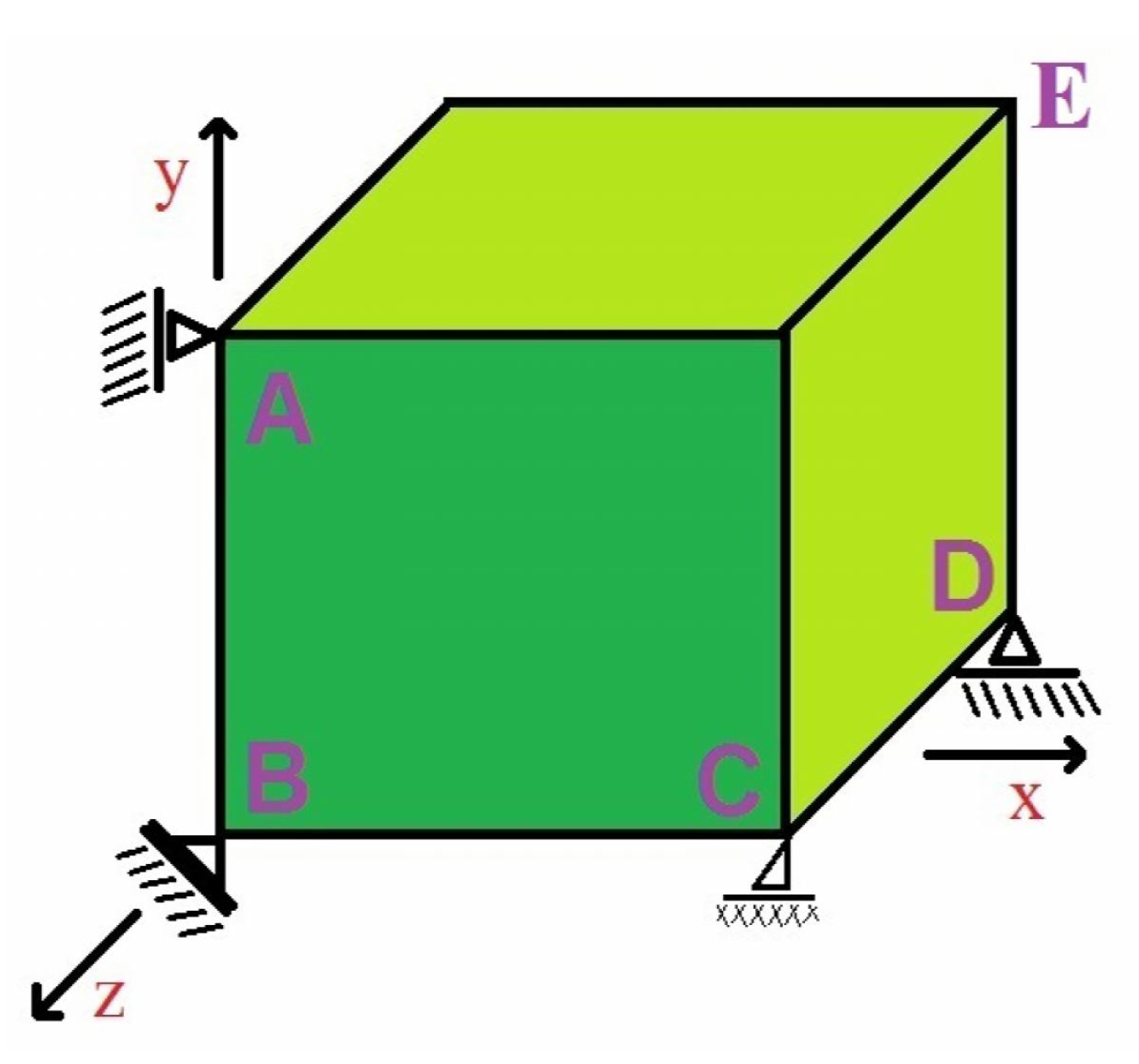
A preliminary study in the following of our previous studies [88,89,90] is on a regular cube, modeled with one 8 node element. The minimal number of freedoms that have to be constrained is six and many combinations are possible. As shown in Figure 2, all three degrees of freedom at point B are fixed. This prevents all rigid body translations, and leaves three rotations to be taken care of. The x displacement component at point A is constrained to prevent rotation about z, and the z component is fixed at point C to prevent rotation about y. The y component is constrained at point D to prevent rotation about x [91].

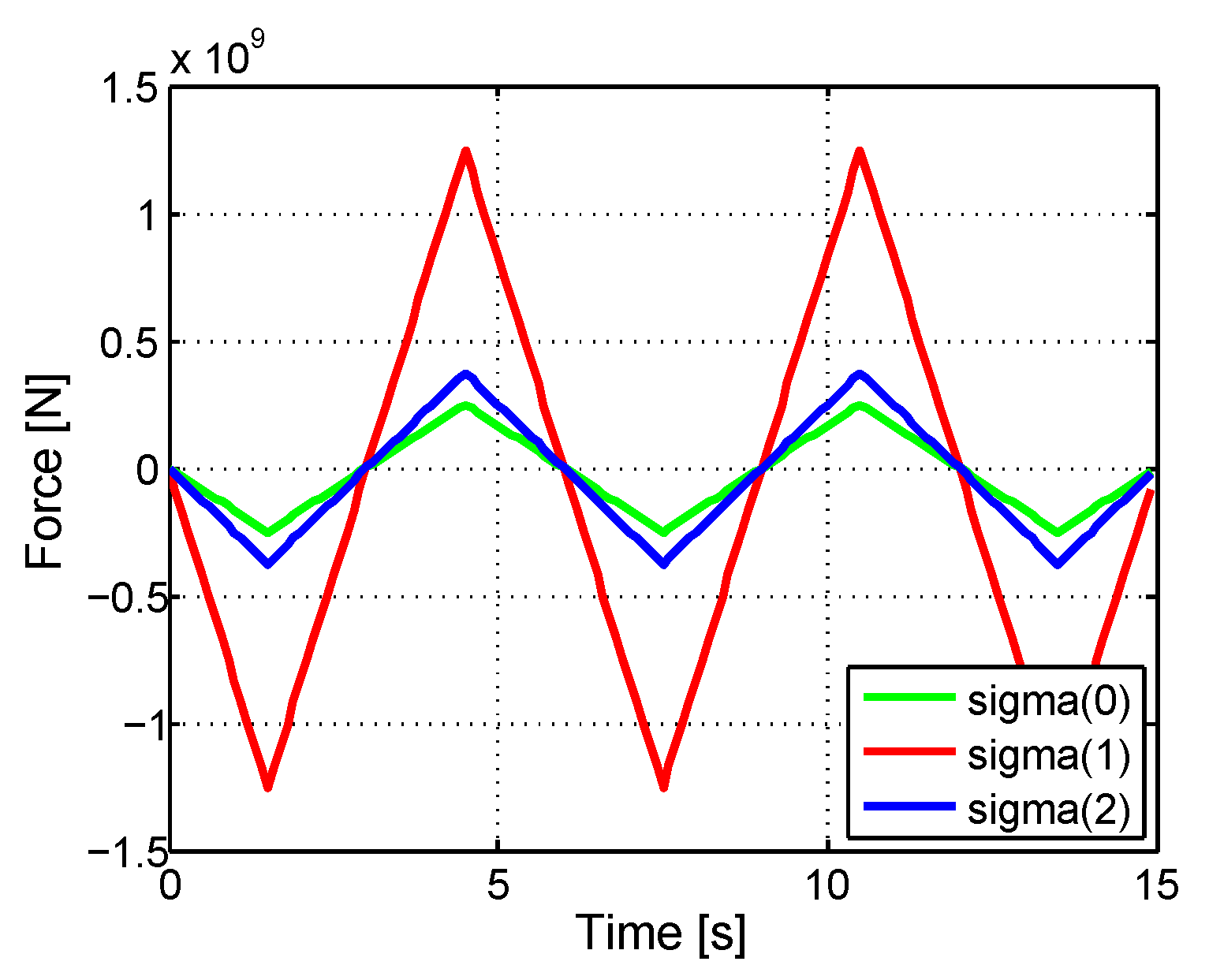
The normal tractions, which is a Neumann boundary condition are applied cyclically in x, y and z directions on front and back faces and the magnitude of tractions in all directions are shown in Figure 3 where green, red and blue colors represent the stress values in x, y and z directions respectively.

By considering the parameters listed in

Table 2. The model parameters.

$\mathit{\kappa }$	G	${\mathit{\sigma }}_{\mathit{y}}$	n	k	${\mathit{b}}_{\mathit{R}}$	${\mathit{H}}_{\mathit{R}}$	${\mathit{b}}_{\mathit{\chi }}$	${\mathit{H}}_{\mathit{\chi }}$
1.66 × 109	7.69 × 108	1.7 × 108	1	1.5 × 108	50	2.75 × 108	50	2.75 × 108

, for the top right corner node on back face, point E, as shown in Figure 2, the related displacement graph is obtained as shown in Figure 4 where green, red and blue colors represent the displacement of point E in x, y and z directions respectively.

The displacements of point E in x, y and z directions are noted as the virtual data in this case.

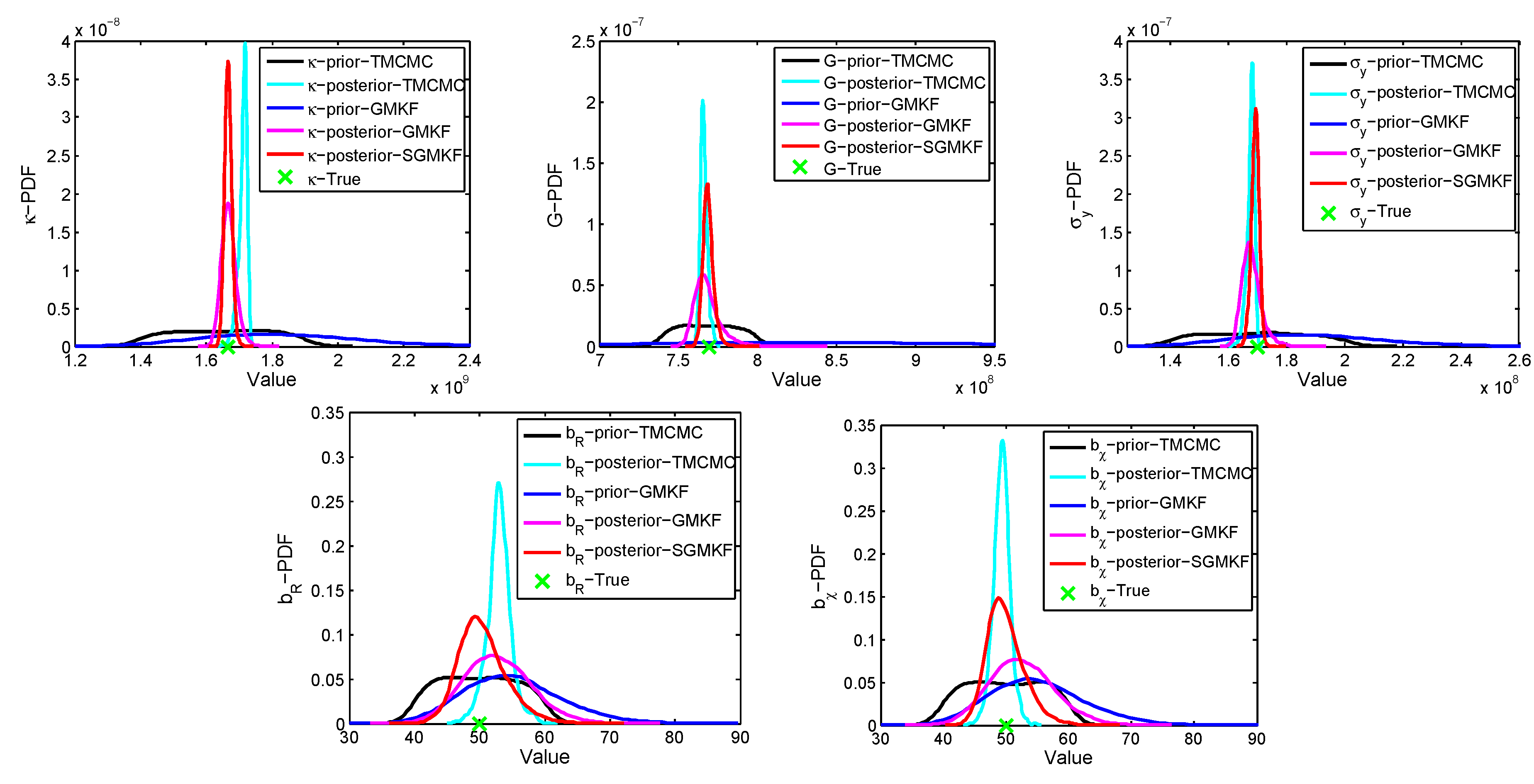
Applying both the stochastic identifications, which are fully discussed in Section 3.1 and Section 3.2, i.e., Transitional Markov Chain monte Carlo method and history matching Gauss-Markov-Kalman filter and sequential Gauss-Markov-Kalman filter approach, the probability density functions of prior and posterior of the identified parameters can be seen and compared in Figure 5. It should be pointed out that in the history matching updating the whole time interval is considered and update is done only once by comparing the predicted value with the recorded displacement history. On the other hand in the sequential updating the process of updating is done several times.

Summarizing the results, the true values and the mean and variance of the estimated parameters for each Bayesian method are compared in

Table 3. The identified model parameters.

Param.	${\mathit{q}}_{\mathbf{true}}$	${\mathit{q}}_{\mathbf{TMCMC}}^{\mathit{m}}$	${\mathit{q}}_{\mathbf{TMCMC}}^{\mathit{std}}$	${\mathit{q}}_{\mathbf{GMKF}}^{\mathit{m}}$	${\mathit{q}}_{\mathbf{GMKF}}^{\mathit{std}}$	${\mathit{q}}_{\mathbf{SGMKF}}^{\mathit{m}}$	${\mathit{q}}_{\mathbf{SGMKF}}^{\mathit{std}}$
$\kappa$	1.66 × 109	1.71 × 109	1.33 × 107	1.66 × 109	2.28 × 107	1.66 × 109	1.13 × 107
G	7.69 × 108	7.66 × 108	2.24 × 106	7.68 × 108	9.09 × 106	7.68 × 108	3.47 × 106
$b_R$	50	53.00	1.83	54.78	5.16	52.36	3.71
$b_{\chi }$	50	49.30	1.32	54.58	5.15	52.04	3.01
${\sigma }_y$	1.7 × 108	1.67 × 108	1.37 × 106	1.67 × 108	3.48 × 106	1.69 × 108	1.35 × 106

.

5. Discussion and Comparison

By comparing the results from the two main approaches, it can be concluded Transitional Markov Chain Monte Carlo and Gauss-Markov-Kalman filter method provide accurate result and identify the known parameters for the viscoplasticity model with isotropic and kinematic hardening behavior except in the history matching update approach as the Gauss-Markov-Kalman filter method for the hardening parameters are not as narrow as the rest of parameter’s distributions as shown in Figure 5. This is because the hardening parameters have no direct and strong influence on the measured displacement and so the uncertainties are not reduced good enough than rest of the parameters as there is no enough information. As another reason it can be mentioned that updating is done only once when history matching Gauss-Markov-Kalman filter is applied and hence the posterior distributions of hardening parameters are not as narrow as when sequential Gauss-Markov-Kalman filter is employed.

In addition, as the computations are evaluated from the initial time step after each update in the sequential Gauss-Markov-Kalman filter, more information is recorded in total. Therefore, better identification and reduction of uncertainty can be obtained in comparison with history matching Gauss-Markov-Kalman filter.

There is not much difference between the standard deviation of the uncertain parameters between Transitional Markov Chain Monte Carlo approach and Gauss-Markov-Kalman filter approach for sequential updating of viscoplasticity with isotropic and kinematic hardening behavior. It should also be noted that the Transitional Markov Chain Monte Carlo method computational time is significantly higher than the other approach. The computational time is more in the Gauss-Markov-Kalman filter approach as multiple updating is involved in the sequential updating of Gauss-Markov-Kalman filter approach.

As Transitional Markov Chain Monte Carlo approach applied on viscoplasticity model with isotropic and kinematic hardening is computationally too much expensive, Gauss-Markov-Kalman filter method is only considered for the viscoplastic-damage model in Section 5.1.

5.1. Validation Procedure on Viscoplastic-Damage Model with Isotropic and Kinematic Hardening

In this section the capability of only one of the Bayesian approaches discussed in the previous sections is studied. Gauss-Markov-Kalman filter using the polynomial chaos expansion is applied on a viscoplastic-damage model with both the isotropic and kinematic hardening behavior.

The parameters which are set as the uncertain parameters are bulk modulus ($\kappa$), shear modulus (G), the isotropic hardening coefficient ($b_R$), the kinematic hardening coefficient ($b_{\chi }$) and the yield stress (${\sigma }_y$) as well as damage parameters (($c_1$), ($c_2$) and ($c_3$)). Hence the vector of unknown parameters is $\mathit{q}=\left[\kappa \left(\omega \right),G\left(\omega \right),{\sigma }_y\left(\omega \right),b_R\left(\omega \right),b_{\chi }\left(\omega \right),c_1\left(\omega \right),c_2\left(\omega \right),c_3\left(\omega \right)\right]$.

Similar to the previous case, preliminary study is on a regular cube, modeled with one 8 node element as shown in Figure 2. Similarly the same Dirichlet boundary condition is considered. Also the same tractions which is a Neumann boundary condition are applied cyclically in x, y and z directions on front and back faces and the magnitude of tractions in all directions are shown in Figure 6 where green, red and blue colors represent the stress values in x, y and z directions respectively.

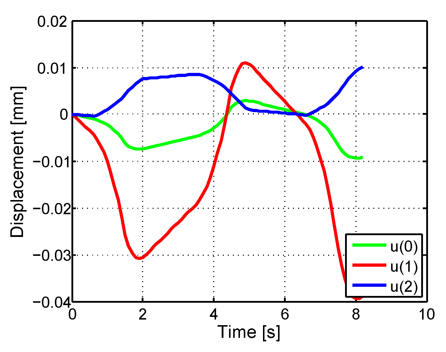
By considering the parameters listed in

Table 4. The model parameters.

$\mathit{\kappa }$	G	${\mathit{\sigma }}_{\mathit{y}}$	n	k	${\mathit{b}}_{\mathit{R}}$	${\mathit{H}}_{\mathit{R}}$	${\mathit{b}}_{\mathit{\chi }}$	${\mathit{H}}_{\mathit{\chi }}$	${\mathit{c}}_1$	${\mathit{c}}_2$	${\mathit{c}}_3$
1.66 × 105	7.69 × 104	266	1	23,500	298.6	117.2	100	150	7	8	−80

, for the top right corner node on back face, point E, as shown in Figure 2, the corresponding displacement graph is obtained as shown in Figure 7 where green, red and blue colors represent the displacement of point E in x, y and z directions respectively.

Again the displacements of point E in x, y and z directions are noted as the virtual data in this case.

Applying the Gauss-Markov-Kalman filter approach, the probability density functions of prior and posterior of the identified parameters can be seen and compared in Figure 8.

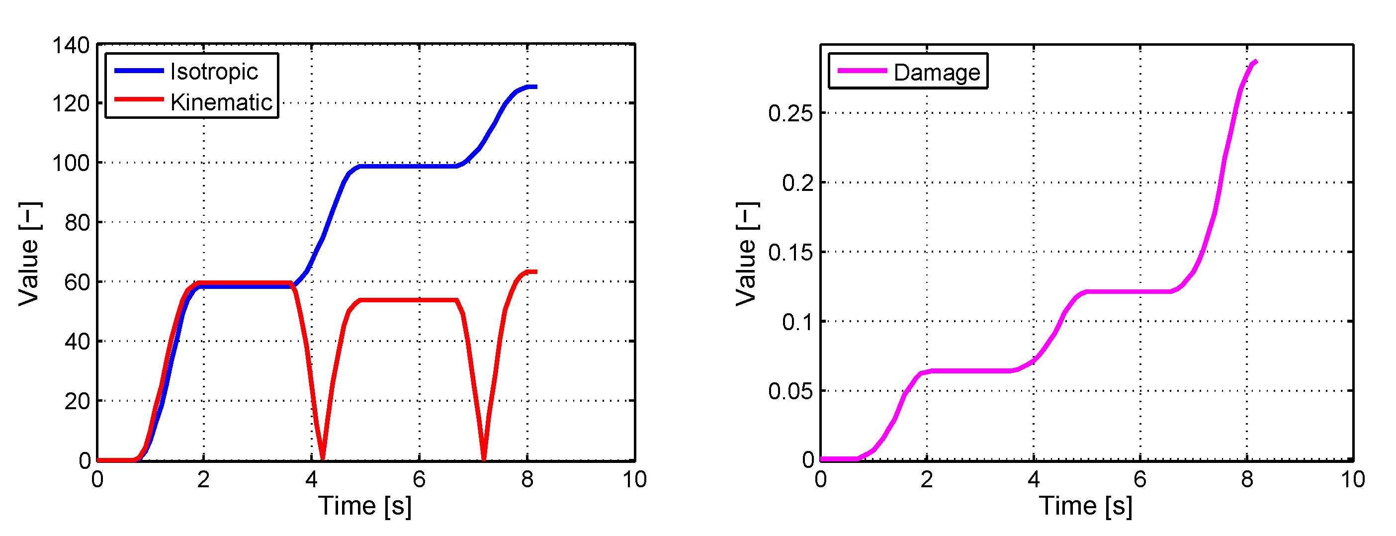
From the sharpness of the posterior PDF of $\kappa$, G and ${\sigma }_y$, it can be concluded that enough information from virtual data is received, and updating the parameters considering their uncertainty is done much easier than the hardening and damage parameters. One reason that can be mentioned is that the process is not always in the states that hardening and damage equations are involved. Therefore less information from the whole simulation can be analyzed to estimate the hardening parameters and update their parameters’ uncertainties. As the evaluation of hardening and local damage are seen in Figure 9, only in the time intervals [0.8 2.0], [3.5 5.0] and [6.6 8.2], and [0.8 2.0] and [6.6 8.2] hardening equations and damage equations are involved respectively. Therefore hardening and damage parameters are updated, but not as much as the rest of the parameters.

Summarizing the results, the true values and the mean and variance of the estimated parameters are compared in

Table 5. The identified model parameters.

Param.	${\mathit{q}}_{\mathbf{true}}$	${\mathit{q}}_{\mathbf{GMKF}}^{\mathit{m}}$	${\mathit{q}}_{\mathbf{GMKF}}^{\mathit{std}}$	${\mathit{q}}_{\mathbf{SGMKF}}^{\mathit{m}}$	${\mathit{q}}_{\mathbf{SGMKF}}^{\mathit{std}}$
$\kappa$	1.66 × 105	1.66 × 105	2.03 × 103	1.66 × 105	937.87
G	7.69 × 104	7.70 × 104	710.34	7.70 × 104	430.05
${\sigma }_y$	266	264.75	1.81	265.1	1.07
$b_R$	298.6	304.75	29.02	300.35	7.06
$b_{\chi }$	100	103.12	11.18	102.98	2.77
$c_1$	7	7.07	0.82	6.84	0.65
$c_2$	8	7.82	0.70	8.13	0.57
$c_3$	−80	−86.29	10.29	−79.98	3.34

.

6. Conclusions

The updating is possible by Gauss-Markov-Kalman filter approach for the viscoplastic-damage model with isotropic and kinematic hardening as the updating is performed according to the history matching or sequentially updating method. However it should be pointed out that for the parameters such as hardening and damage parameters, which do not have much strong influence on the measured displacement than the rest of parameters, the identification can not be done well as compared to the rest of parameters. Hence a better identification is achieved when the more information is available from the measurement.

Moreover the uncertainty of the parameters is reduced in the such a way that the posterior distribution functions of the hardening and damage parameters are not as narrow as the rest parameters for the history matching and sequential updating methods.

The sequential updating needs more computational time as the updating process is performed several times than the history updating approach. By considering the fact that the computations are done from the initial time step after each update which leads to observe more information as well. On the other hand, the identification and reduction of the parameter uncertainty as inferred from the update of the parameters is more accurate and acceptable for the sequential updating method than the history matching update as it is seen from the posterior densities of hardening and damage parameters by both approaches shown in Figure 8.

7. Summary

Using the stochastic methods explained in Section 3 to identify the model parameters of the Chaboche damaged model indicates that it is possible to identify the model parameters using Transitional Markov Chain Monte Carlo method and Gauss-Markov Kalman filter approach by means of history updating and also sequentially although the mentioned methods provide different results and the conclusions are discussed below.

The computational time of the Transitional Markov Chain Monte Carlo method on the mentioned model is very high and this results in no sense of applying this method in the economical point of view on the complicated material models. The sequential Gauss-Markov-Kalman filter approach for both variety of the considered models is not as fast as the history matching approach as updating is done multiple times. But still the computation time needed is reasonable and acceptable as a stochastic approach to identify the parameters of a PDE system.

A considerable difference in results is observed between the updated random variables of the uncertain parameters for the considered models which are determined by employing the Gauss-Markov-Kalman filter approach. This is because of the fact that the hardening and damage parameters do not have a strong and direct influence as like the bulk modulus, shear modulus and the yield stress which have a dominant influence on the considered measured displacement output data.

The Gauss-Markov-Kalman filter approach in a history matching update approach is not an optimized method to identify the parameters of the viscoplasticity which includes hardening model and viscoplastic-damage model. This is because, the hardening and damage parameters are not identified well and their uncertainties are not properly reduced as updating is done only once. Further, it is also to be noted that the number of observed states where the bulk modulus, shear modulus and yield stress are involved and identifiable, i.e., the number of states where the elasticity and plasticity part are involved and identifiable are more than the number of states where the hardening and damage parameters are involved and identifiable i.e., only plasticity part.

Based on the reliability, accuracy and computational time, the most suitable method among the employed methods is the sequential Gauss-Markov-Kalman filter approach for the viscoplastic model with isotropic and kinematic hardening and also for the viscoplastic-damage model enriched with hardening behavior. The parameters such as hardening parameters, damage parameters, bulk modulus, shear modulus and yield stress are well updated and posterior distributions representing their uncertainties are much narrow for these parameters. Using sequential Gauss-Markov-Kalman filter approach the parameters should be updated at proper time intervals to save time and to reduce cost. Lesser number of updates results in lesser computation time. Hence particular times should be selected to identify the parameters as discussed in Section 4 where the hardening and damage parameters are changing continuously. Considering this fact results in a better parameter identification and better reduction of parameter uncertainties in a very less time.

It should be noted that the damage evolution has been restricted in such a way that non-local damage should not exceed certain value, i.e., only minor damage is considered for the Gauss-Markov-Kalman filter approach on a viscoplastic-damage model to identify its parameters. Obviously the damage parameters are identified better by using the Gauss-Markov-Kalman filter approach when an immense damage is considered, i.e., the measured displacement data is influenced more by a bigger damage and results in better identification of damage parameters from the provided data. Considering the mentioned fact, this study proves that identification of the model and damage parameters are possible using Bayesian methods before the specimen is really damaged and completely collapsed. Such a Bayesian approach can be recommended to be applied for mechanical structure health monitoring [92,93].

References

1. Adeli, E.; Rosić, B.V.; Matthies, H.G.; Reinstädler, S.; Dinkler, D. Comparison of Bayesian Methods on Parameter Identification for a Viscoplastic Model with Damage. J. Comput. Mech. 2019. [Google Scholar] [CrossRef]
2. Pacheco, C.; Dulikravich, G.S.; Vesenjak, M.; Borovinsek, M.; Duarte, I.M.A.; Jha, R.; Reddy, S.R.; Orlande, H.R.B.; Colaco, M.J. Inverse parameter identification in solid mechanics using Bayesian statistics, response surfaces and minimization. Tech. Mech. 2016, 36, 120–131. [Google Scholar]
3. Słonski, M. Bayesian identification of elastic parameters in composite laminates applying lamb waves monitoring. In Proceedings of the Fifth ECCOMAS Thematic Conference on Computational Methods in Structural Dynamics and Earthquake Engineering, Crete Island, Greece, 25–27 May 2015. [Google Scholar]
4. Zhang, E.; Chazot, J.D.; Antoni, J. Parametric identification of elastic modulus of polymeric material in laminated glasses. In Proceedings of the 16th IFAC Symposium on System Identification, The International Federation of Automatic Control, Brussels, Belgium, 11–13 July 2012. [Google Scholar]
5. Gallina, A.; Ambrozinski, L.; Packo, P.; Pieczonka, L.; Uhl, T.; Staszewski, W.J. Bayesian parameter identification of orthotropic composite materials using lamb waves dispersion curves measurement. J. Vibr. Control 2017, 23, 2656–2671. [Google Scholar] [CrossRef]
6. Pieczonka, L.; Gallina, A.; Ambrozinski, L.; Packo, P.; Uhl, T.; Staszewski, W.J. Parameters identification of composite materials using Bayesian approach and guided ultrasonic waves. In Proceedings of the ISMA 2016—International Conference on Noise and Vibration Engineering and USD2016, Leuven, Belgium, 19–21 September 2016. [Google Scholar]
7. Arnst, M.; Ghanem, R.; Soize, C. Identification of Bayesian posteriors for coefficients of chaos expansions. J. Comput. Phys. 2010, 229, 3134–3154. [Google Scholar] [CrossRef] [Green Version]
8. Rappel, H.; Beex, L.A.A.; Noels, L.; Bordas, S.P.A. Identifying elastoplastic parameters with Bayes’ theorem considering double error sources and model uncertainty. J. Prob. Eng. Mech. 2018. [Google Scholar] [CrossRef] [Green Version]
9. An, D.; Cho, J.; Kim, N.H. Identification of correlated damage parameters under noise and bias using Bayesian inference. Struct. Health Monit. 2011, 11, 293–303. [Google Scholar] [CrossRef]
10. Hernandez, W.P.; Borges, F.C.L.; Castello, D.A.; Roitman, N.; Magluta, C. Bayesian inference applied on model calibration of a fractional derivative viscoelastic model. In Proceedings of the XVII International Symposium on Dynamic Problems of Mechanics, Natal, Brazil, 22–27 February 2015. [Google Scholar]
11. Mahnken, R. Identification of material parameters for constitutive equations. In Encyclopedia of Computational Mechanics, 2nd ed.; Part 2. Solids and Structures; John Wiley & Sons, Ltd.: Hoboken, NJ, USA, 2017; pp. 1–21. [Google Scholar]
12. Zheng, W.; Yu, Y. Bayesian probabilistic framework for damage identification of steel truss bridges under joint uncertainties. Adv. Civ. Eng. 2013, 1–13. [Google Scholar] [CrossRef]
13. Nichols, J.M.; Moore, E.Z.; Murphy, K.D. Bayesian identification of a cracked plate using a population-based Markov Chain Monte Carlo method. J. Comput. Struct. 2011, 89, 1323–1332. [Google Scholar] [CrossRef]
14. Madireddy, S.; Sista, B.; Vemaganti, K. A Bayesian approach to selecting hyperelastic constitutive models of soft tissue. J. Comput. Appl. Math. 2015, 291, 102–122. [Google Scholar] [CrossRef]
15. Wang, J.; Zabaras, N. A Bayesian inference approach to the inverse heat conduction problem. Int. J. Heat Mass Trans. 2004, 47, 3927–3941. [Google Scholar] [CrossRef]
16. Oh, C.K.; Beck, J.L.; Yamada, M. Bayesian learning using automatic relevance determination prior with an application to earthquake early warning. J. Eng. Mech. 2008, 134, 1013–1020. [Google Scholar] [CrossRef] [Green Version]
17. Alvin, K. Finite element model update via Bayesian estimation and minimization of dynamic residuals. Am. Inst. Aeronaut. Astronaut. J. 1997, 135, 879–886. [Google Scholar] [CrossRef] [Green Version]
18. Marwala, T.; Sibusiso, S. Finite element model updating using Bayesian framework and modal properties. J. Aircraft 2005, 42, 275–278. [Google Scholar] [CrossRef]
19. Daghia, F.; de Miranda, S.; Ubertini, F.; Viola, E. Estimation of elastic constants of thick laminated plates within a Bayesian framework. J. Compos. Struct. 2007, 80, 461–473. [Google Scholar] [CrossRef]
20. Abhinav, S.; Manohar, C. Bayesian parameter identification in dynamic state space models using modified measurement equations. Int. J. Non-Linear Mech. 2015, 71, 89–103. [Google Scholar] [CrossRef]
21. Gogu, C.; Yin, W.; Haftka, R.; Ifju, P.; Molimard, J.; le Riche, R.; Vautrin, A. Bayesian identification of elastic constants in multi-directional laminate from Moire interferometry displacement fields. J. Exp. Mech. 2013, 53, 635–648. [Google Scholar] [CrossRef] [Green Version]
22. Gogu, C.; Haftka, R.; Molimard, J.; Vautrin, A. Introduction to the Bayesian approach applied to elastic constants identification. Am. Inst. Aeronaut. Astronaut. J. 2010, 48, 893–903. [Google Scholar] [CrossRef]
23. Koutsourelakis, P.S. A novel Bayesian strategy for the identification of spatially varying material properties and model validation: An application to static elastography. Int. J. Num. Methods Eng. 2012, 91, 249–268. [Google Scholar] [CrossRef] [Green Version]
24. Koutsourelakis, P.S. A multi-resolution, non-parametric, Bayesian framework for identification of spatially-varying model parameters. J. Comput. Phys. 2009, 228, 6184–6211. [Google Scholar] [CrossRef] [Green Version]
25. Fitzenz, D.D.; Jalobeanu, A.; Hickman, S.H. Integrating laboratory creep compaction data with numerical fault models: A Bayesian framework. J. Geophys. Res. Solid Earth 2007, 112, B08410. [Google Scholar] [CrossRef]
26. Most, T. Identification of the parameters of complex constitutive models: Least squares minimization vs. Bayesian updating. In Reliability and Optimization of Structural Systems; Straub, D., Ed.; CRC Press: Boca Raton, FL, USA, 2010; pp. 119–130. [Google Scholar]
27. Sarkar, S.; Kosson, D.S.; Mahadevan, S.; Meeussen, J.C.L.; Sloot, H.v.; Arnold, J.R.; Brown, K.G. Bayesian calibration of thermodynamic parameters for geochemical speciation modeling of cementitious materials. J. Cement Concr. Res. 2012, 42, 889–902. [Google Scholar] [CrossRef]
28. Zhang, E.; Chazot, J.D.; Antoni, J.; Hamdi, M. Bayesian characterization of Young’s modulus of viscoelastic materials in laminated structures. J. Sound Vibr. 2013, 332, 3654–3666. [Google Scholar] [CrossRef]
29. Mehrez, L.; Kassem, E.; Masad, E.; Little, D. Stochastic identification of linear-viscoelastic models of aged and unaged asphalt mixtures. J. Mater. Civ. Eng. 2015, 27, 04014149. [Google Scholar] [CrossRef]
30. Miles, P.; Hays, M.; Smith, R.; Oates, W. Bayesian uncertainty analysis of finite deformation viscoelasticity. J. Mech. Mater. 2015, 91, 35–49. [Google Scholar] [CrossRef] [Green Version]
31. Zhao, X.; Pelegri, A.A. A Bayesian approach for characterization of soft tissue viscoelasticity in acoustic radiation force imaging. Int. J. Num. Methods Biomed. Eng. 2016, 32, E02741. [Google Scholar] [CrossRef] [PubMed]
32. Kenz, Z.R.; Banks, H.T.; Smith, R.C. Comparison of frequentist and Bayesian confidence analysis methods on a viscoelastic stenosis model. SIAM/ASA J. Uncertain. Quant. 2013, 1, 348–369. [Google Scholar] [CrossRef] [Green Version]
33. An, D.; Choi, J.; Kim, N.H.; Pattabhiraman, S. Fatigue life prediction based on Bayesian approach to incorporate field data into probability model. J. Struct. Eng. Mech. 2011, 37, 427–442. [Google Scholar] [CrossRef] [Green Version]
34. Hoshi, T.; Kobayashi, Y.; Kawamura, K.; Fujie, M.G. Developing an intraoperative methodology using the finite element method and the extended Kalman filter to identify the material parameters of an organ model. In Proceedings of the 29th Annual International Conference of the IEEE EMBS Cité Internationale, Lyon, France, 23–26 August 2007. [Google Scholar]
35. Furukawa, T.; Pan, J.W. Stochastic identification of elastic constants for anisotropic materials. Int. J. Num. Methods Eng. 2010, 81, 429–452. [Google Scholar] [CrossRef]
36. Conte, J.P.; Astroza, R.; Ebrahimian, H. Bayesian methods for nonlinear system identification of civil structures. MATEC Web Conf. 2015, 24, 03002. [Google Scholar] [CrossRef]
37. Hendriks, M.A.N. Identification of the Mechanical Behavior of Solid Materials. Ph.D. Thesis, Department of Mechanical Engineering, Technische Universiteit Eindhoven, Eindhoven, The Netherlands, 1991. [Google Scholar]
38. Bolzon, G.; Fedele, R.; Maier, G. Parameter identification of a cohesive crack model by Kalman filter. J. Comput. Methods Appl. Mech. Eng. 2002, 191, 2847–2871. [Google Scholar] [CrossRef]
39. Astroza, R.; Nguyen, L.T.; Nestorović, T. Finite element model updating using simulated annealing hybridized with unscented Kalman filter. J. Comput. Struct. 2016, 177, 176–191. [Google Scholar] [CrossRef]
40. Mahmoudi, E.; König, M.; Schanz, T. Probabilistic analysis of a gas storage cavity mined in a spatially random rock salt medium. In Proceedings of the Coupled Problems 2017, Rhodes, Greece, 12–14 June 2017. [Google Scholar]
41. Mahmoudi, E.; Khaledi, K.; König, D.; Schanz, T. Probabilistic analysis of a rock salt cavern with application to energy storage systems, using subset simulation methodology. In Energy Geotechnics; Wuttke, F., Bauer, S., Sanchez, M., Eds.; CRC Press: Boca Rotan, FL, USA, 2016; pp. 609–615. [Google Scholar]
42. Wall, O.; Holst, J. Estimation of parameters in viscoplastic and creep material models. SIAM J. Appl. Math. 2001, 61, 2080–2103. [Google Scholar] [CrossRef]
43. Nakamura, T.; Gu, Y. Identification of elastic-plastic anisotropic parameters using instrumented indentation and inverse analysis. J. Mech. Mater. 2007, 39, 340–356. [Google Scholar] [CrossRef]
44. Agmell, M.; Ahadi, A.; Stahl, J. Identification of plasticity constants from orthogonal cutting and inverse analysis. J. Mech. Mater. 2014, 77, 43–51. [Google Scholar] [CrossRef]
45. Sevieri, G.; Andreini, M.; Falco, A.D.; Matthies, H.G. Concrete gravity dams model parameters updating using static measurements. Eng. Struct. 2019, 196. [Google Scholar] [CrossRef]
46. Sevieri, G.; Falco, A.D. Dynamic structural health monitoring for concrete gravity dams based on the Bayesian inference. J. Civil Struct. Health Monit. 2020, 10, 235–250. [Google Scholar] [CrossRef] [Green Version]
47. Sevieri, G.; Falco, A.D.; Marmo, G. Shedding Light on the Effect of Uncertainties in the Seismic Fragility Analysis of Existing Concrete Dams. Infrastructures 2020, 5, 22. [Google Scholar] [CrossRef] [Green Version]
48. Marsili, F.; Croce, P.; Friedman, N.; Formichi, P.; Landi, F. Seismic reliability assessment of a concrete water tank based on the Bayesian updating of the finite element model. ASCE-ASME J. Risk Uncertain. Eng. Syst. Part B Mech. Eng. 2017, 3, 021004. [Google Scholar] [CrossRef]
49. Marsili, F.; Croce, P.; Friedman, N.; Formichi, P.; Landi, F. On Bayesian identification methods for the analysis of existing structures. In Proceedings of the IABSE Congress Stockholm, Challenges in Design and Construction of an Innovative and Sustainable Built Environment, Stockholm, Sweden, 21–23 September 2016; pp. 116–123. [Google Scholar]
50. Croce, P.; Landi, F.; Formichi, P. Probabilistic Seismic Assessment of Existing Masonry Buildings. Buildings 2019, 9, 237. [Google Scholar] [CrossRef] [Green Version]
51. Croce, P.; Formichi, P.; Landi, F. A Bayesian hierarchical model for climatic loads under climate change. Eccomas Proc. UNCECOMP 2019, 298–308. [Google Scholar] [CrossRef] [Green Version]
52. Croce, P.; Marsili, F.; Klawonn, F.; Formichi, P.; Landi, F. Evaluation of statistical parameters of concrete strength from secondary experimental test data. Constr. Build. Mater. 2018, 163, 343–359. [Google Scholar] [CrossRef]
53. Bocciarelli, M.; Bolzon, G.; Maier, G. A constitutive model of metal-ceramic functionally graded material behavior: Formulation and parameter identification. J. Comput. Mater. Sci. 2008, 43, 16–26. [Google Scholar] [CrossRef]
54. Gu, Y.; Nakamura, T.; Prchlik, L.; Sampath, S.; Wallace, J. Micro-indentation and inverse analysis to characterize elastic-plastic graded materials. J. Mater. Sci. Eng. A 2003, 345, 223–233. [Google Scholar] [CrossRef]
55. Corigliano, A.; Mariani, S. Parameter identification of a time-dependent elastic-damage interface model for the simulation of debonding in composites. J. Compos. Sci. Technol. 2001, 61, 191–203. [Google Scholar] [CrossRef]
56. Corigliano, A.; Mariani, S. Simulation of damage in composites by means of interface models: Parameter identification. J. Compos. Sci. Technol. 2001, 61, 2299–2315. [Google Scholar] [CrossRef]
57. Ebrahimian, H.; Astroza, R.; Conte, J.P.; de Callafon, R.A. Nonlinear finite element model updating for damage identification of civil structures using batch Bayesian estimation. J. Mech. Syst. Signal Process. 2017, 84, 194–222. [Google Scholar] [CrossRef]
58. Ebrahimian, H.; Astroza, R.; Conte, J.P. Parametric Identification of Hysteretic Material Constitutive Laws in Nonlinear Finite Element Models using Extended Kalman Filter; Department of Structural Engineering, University of California: San Diego, CA, USA, 2014. [Google Scholar]
59. Ebrahimian, H.; Astroza, R.; Conte, J.P. Extended Kalman filter for material parameter estimation in nonlinear structural finite element models using direct differentiation method. Earthq. Eng. Struct. Dyn. 2015, 44, 1495–1522. [Google Scholar] [CrossRef]
60. Astroza, R.; Ebrahimian, H.; Conte, J.P. Material parameter identification in distributed plasticity FE models of frame-type structures using nonlinear stochastic filtering. J. Eng. Mech. 2015, 141, 04014149. [Google Scholar] [CrossRef]
61. Hariri-Ardebili, M.A.; Heshmati, M.; Boodagh, P.; Salamon, J.W. Probabilistic Identification of Seismic Response Mechanism in a Class of Similar Arch Dams. Infrastructures 2019, 4, 44. [Google Scholar] [CrossRef] [Green Version]
62. Saouma, V.E.; Hariri-Ardebili, M.A. Probabilistic Cracking, Aging and Shaking of Concrete Dams. In Proceedings of the 5th International Symposiumon Dam Safety, Istanbul, Turkey, 27–31 October 2018; pp. 44–56. [Google Scholar]
63. Yan, A.; de Boe, P.; Golinval, J. Structural damage diagnosis by Kalman model based on stochastic subspace identification. Int. J. Struct. Health Monit. 2004, 3, 103–119. [Google Scholar] [CrossRef]
64. Ghannadi, P.; Kourehli, S.S. Model updating and damage detection in multi-story shear frames using salp swarm algorithm. Earthq. Struct. 2019, 17, 63–73. [Google Scholar]
65. Ghannadi, P.; Kourehli, S.S.; Noori, M.; Altabey, W.A. Efficiency of grey wolf optimization algorithm for damage detection of skeletal structures via expanded mode shapes. Adv. Struct. Eng. 2020. [Google Scholar] [CrossRef]
66. Gharehbaghi, V.; Nguyen, A.; Farsangi, E.N.; Yang, T.Y. Supervised damage and deterioration detection in building structures using an enhanced autoregressive time-series approach. J. Build. Eng. 2020. [Google Scholar] [CrossRef]
67. Ching, J.; Chen, Y.C. Transitional Markov Chain Monte Carlo method for Bayesian model updating, model class selection and model averaging. J. Eng. Mech. 2007, 133, 816–832. [Google Scholar] [CrossRef]
68. Ching, J.; Wang, J. Application of the Transitional Markov Chain Monte Carlo algorithm to probabilistic site characterization. J. Eng. Geol. 2016, 203, 151–167. [Google Scholar] [CrossRef]
69. Matthies, H.G.; Zander, E.; Rosić, B.V.; Litvinenko, A.; Pajonk, O. Inverse problems in a Bayesian setting. J. Comput. Methods Solids Fluids 2016, 245–286. [Google Scholar]
70. Matthies, H.G.; Zander, E.; Rosić, B.V.; Litvinenko, A. Parameter estimation via conditional expectation: A Bayesian inversion. Adv. Model. Simulat. Eng. Sci. 2016, 3, 24. [Google Scholar] [CrossRef] [Green Version]
71. Matthies, H.G.; Litvinenko, A.; Rosić, B.V.; Zander, E. Bayesian parameter estimation via filtering and functional approximations. Tech. Gazette 2016, 23, 1–8. [Google Scholar]
72. Pajonk, O.; Rosić, B.V.; Litvinenko, A.; Matthies, H.G. A deterministic filter for non-Gaussian Bayesian estimation—Applications to dynamical system estimation with noisy measurements. Phys. D Nonlinear Phenomena 2012, 241, 775–788. [Google Scholar] [CrossRef]
73. Simo, J.C.; Hughes, T.J.R. Computational Inelasticity, 7th ed.; Springer: New York, NY, USA, 1998. [Google Scholar]
74. Kowalsky, U.; Meyer, J.; Heinrich, S.; Dinkler, D. A nonlocal damage model for mild steel under inelastic cyclic straining. Comput. Mater. Sci. 2012, 63, 28–34. [Google Scholar] [CrossRef]
75. Pirondi, A.; Bonora, N. Modeling ductile damage under fully reversed cycling. Comput. Mater. Sci. 2003, 26, 129–141. [Google Scholar] [CrossRef]
76. Hughes, T.; Hulbert, G. Space-time finite element methods for elastodynamics: Formulations and error estimates. Comput. Methods Appl. Mech. Eng. 1988, 66, 339–363. [Google Scholar] [CrossRef]
77. Zienkiewicz, O.C.; Taylor, R.L.; Zhu, J.Z. The Finite Element Method: Its Basis and Fundamentals, 6th ed.; Elsevier Butterworth-Heinemann: Oxford, UK, 2005; ISBN 978-1-85617-633-0. [Google Scholar]
78. Wang, J.; Katafygiotis, L.S.; Noori, M.N. Transitional Markov Chain Monte Carlo simulation for reliability-based optimization. In Safety, Reliability, Risk and Life-Cycle Performance of Structures & Infrastructures; Deodatis, G., Ellingwood, B.R., Frangopol, D.M., Eds.; CRC Press: Boca Raton, FL, USA, 2014; pp. 1593–1599. [Google Scholar]
79. McGrayne, S.B. The Theory That Would Not Die; Yale University Press: New Haven, CT, USA, 2011. [Google Scholar]
80. Luenberger, D.G. Optimization by Vector Space Methods; Wiley: Chichester, UK, 1969. [Google Scholar]
81. Grewal, M.S.; Andrews, A.P. Kalman Filtering: Theory and Practice Using MATLAB; Wiley: Chichester, UK, 2008. [Google Scholar]
82. Evensen, G. Data Assimilation—The Ensemble Kalman Filter; Springer: Berlin/Heidelberg, Germany, 2009. [Google Scholar]
83. Pajonk, O. Stochastic Spectral Methods for Linear Bayesian Inference. Ph.D. Thesis, Institut für Wissenschaftliches Rechnen, Technische Universität Braunschweig, Braunschweig, Germany, 2012. [Google Scholar]
84. Matthies, H.G. Stochastic finite elements: Computational Approaches to Stochastic Partial Differential Equations. J. Appl. Math. Mech. 2008, 88, 849–873. [Google Scholar] [CrossRef]
85. Xiu, D. Numerical Methods for Stochastic Computations: A Spectral Method Approach; Princeton University Press: Princeton, NJ, USA, 2010. [Google Scholar]
86. Wiener, N. The homogeneous chaos. Am. J. Math. 1938, 60, 897–936. [Google Scholar] [CrossRef]
87. Ghanem, R.; Spanos, P.D. Stochastic Finite Eements—A Spectral Approach; Springer: Berlin/Heidelberg, Germany, 1991. [Google Scholar]
88. Adeli, E.; Rosić, B.V.; Matthies, H.G.; Reinstädler, S. Bayesian parameter identification in plasticity. In Proceedings of the XIV International Conference on Computational Plasticity, Fundamentals and Applications COMPLAS XIV, Barcelona, Spain, 5–7 September 2017. [Google Scholar]
89. Adeli, E.; Rosić, B.V.; Matthies, H.G.; Reinstädler, S. Effect of Load Path on Parameter Identification for Plasticity Models using Bayesian Methods. In Lecture Notes in Computational Science and Engineering; Nature Springer, 2018; Available online: http://arxiv.org/abs/1906.07246 (accessed on 17 June 2019).
90. Adeli, E.; Matthies, H.G. Parameter Identification in Viscoplasticity using Transitional Markov Chain Monte Carlo Method. Available online: http://arxiv.org/abs/1906.10647 (accessed on 21 June 2019).
91. Felippa, C. Introduction to FEM, FEM Modeling: Mesh, Loads and BCs; University of Colorado: Boulder, CO, USA, 2016. [Google Scholar]
92. Adeli, E. Viscoplastic-Damage Model Parameter Identification via Bayesian Methods. Ph.D. Dissertation, Institut für Wissenschaftliches Rechnen, Technische Universität Braunschweig, Braunschweig, Germany, 2019. [Google Scholar] [CrossRef]
93. Adeli, E.; Rosić, B.V.; Matthies, H.G.; Reinstädler, S.; Dinkler, D. Bayesian Parameter Determination of a CT-Test Described by a Viscoplastic-Damage Model Considering the Model Error. 2019. Available online: https://www.researchgate.net/publication/334537857_Bayesian_Parameter_Determination_of_a_CT-Test_described_by_a_Viscoplastic-Damage_Model_considering_the_Model_Error (accessed on 21 June 2019).
94. Bonet, J.; Wood, R.D. Nonlinear Continuum Mechanics for Finite Element Analysis; Cambridge University Press: Cambridge, UK, 1997; ISBN 9780521572729. [Google Scholar]
95. Chaboche, J.L.; Rousselier, G. On the plastic and viscoplastic constitutive equations—Part 1: Rules developed with internal variable concept. J. Press. Vessel Technol. 1983, 105, 153–158. [Google Scholar] [CrossRef]
96. Chaboche, J.L.; Rousselier, G. On the plastic and viscoplastic constitutive equations—Part 2: Application of internal variable concepts to the 316 stainless steel. J. Press. Vessel Technol. 1983, 105, 159–164. [Google Scholar] [CrossRef]
97. Bobrowski, A. Functional Analysis for Probability and Stochastic Processes; Cambridge University Press: Cambridge, UK, 2005. [Google Scholar]
98. Pritchard, C. The Changing Shape of Geomtetry; Cambridge University Press: Cambridge, UK, 2003. [Google Scholar]
99. Rao, M. Conditional Measures and Applications; CRC Press: Boca Raton, FL, USA, 2005. [Google Scholar]
100. Rao, M.; Swift, R.J. Probability Theory with Applications. Mathematics and Its Applications, Band 582; Springer: Berlin/Heidelberg, Germany, 2006. [Google Scholar]
101. Tarantola, A. Inverse Problem Theory and Methods for Model Parameter Estimation; SIAM: Philadelphia, PA, USA, 2004. [Google Scholar]
102. Jaynes, E.T. Probability Theory, the Logic of Science; Cambridge University Press: Cambridge, UK, 2003. [Google Scholar]
103. Aster, R.C.; Borchers, B.; Thurber, C.H. Parameter Estimation and Inverse Problems, 2nd ed.; Academic Press: Cambridge, MA, USA, 2012; ISBN 978-0-12-804651-7. [Google Scholar]
104. Dashti, M.; Stuart, A.M. The Bayesian Approach to Inverse Problems. In Handbook of Uncertainty Quantification; Springer Nature: Cham, Switzerland, 2015; pp. 1–118. [Google Scholar]
105. Bosq, D. Linear processes in function spaces, theory and applications. In Lecture Notes in Statistics 149; Springer: Berlin/Heidelberg, Germany, 2000. [Google Scholar]
Figure 1. Sequential GMKF method.
Metals 10 00876 g001
Figure 2. Boundary condition considered.
Metals 10 00876 g002
Figure 3. Decomposed applied force at point E according to time.
Metals 10 00876 g003
Figure 4. Displacement of point E in x, y and z directions according to time.
Metals 10 00876 g004
Figure 5. PDF of identified parameters.
Metals 10 00876 g005
Figure 6. Decomposed applied force at point E according to time.
Metals 10 00876 g006
Figure 7. Displacement of point E in x, y and z directions according to time.
Metals 10 00876 g007
Figure 8. PDF of identified parameters.
Metals 10 00876 g008
Figure 9. Isotropic and kinematic hardenings- and local damage evaluation according to time [s].
Metals 10 00876 g009