A Comparative Assessment of Six Machine Learning Models for Prediction of Bending Force in Hot Strip Rolling Process

Abstract

In the hot strip rolling (HSR) process, accurate prediction of bending force can improve the control accuracy of the strip crown and flatness, and further improve the strip shape quality. In this paper, six machine learning models, including Artificial Neural Network (ANN), Support Vector Machine (SVR), Classification and Regression Tree (CART), Bagging Regression Tree (BRT), Least Absolute Shrinkage and Selection operator (LASSO), and Gaussian Process Regression (GPR), were applied to predict the bending force in the HSR process. A comparative experiment was carried out based on a real-life dataset, and the prediction performance of the six models was analyzed from prediction accuracy, stability, and computational cost. The prediction performance of the six models was assessed using three evaluation metrics of root mean square error (RMSE), mean absolute error (MAE), and coefficient of determination (R²). The results show that the GPR model is considered as the optimal model for bending force prediction with the best prediction accuracy, better stability, and acceptable computational cost. The prediction accuracy and stability of CART and ANN are slightly lower than that of GPR. Although BRT also shows a good combination of prediction accuracy and computational cost, the stability of BRT is the worst in the six models. SVM not only has poor prediction accuracy, but also has the highest computational cost while LASSO showed the worst prediction accuracy.

1. Introduction

In recent years, with the development of hot strip rolling (HSR) technology, product users continuously call for increased requirements. These increased requirements include strip variety, specifications, and strip shape quality. A good strip shape quality produced by the HSR process has a desired crown and flatness, and it is also an important factor to determine the competitiveness of strip in the market. Therefore, strip shape quality has become a hot topic of many scholars [1,2].

There are many factors that affect the strip shape quality, which are mainly related to the roller, strip, and rolling conditions in the HSR process. However, the field environment of the rolling process is very complex, and there are many factors that affect the strip shape quality. There is still no perfect solution to the strip shape quality problem in the world. In order to improve the strip shape quality, most scholars mainly studied the following two aspects. The research on production equipment is the first thought of researchers. In order to improve strip shape quality, it is necessary to control roll crown effectively. Therefore, it can be achieved by replacing the work rolls with ultra-high strength and ultra-high hardness to reduce the flexural deformation of the rolls. Secondly, the research on rolling technology has been carried out. In order to improve the precision of the preset model and compensate the influence of external factors on strip shape measurement precision, various factors affecting shape control model were studied. For example, in the process of strip production, if the detection accuracy of the roller is too low, it will directly affect the adjustment ability of the strip shape control mechanism, so the strip shape quality could not be improved [1,3].

Hydraulic roll bending control is one of the main methods to control the shape of hot rolled strip. The hydraulic roll bending system is more and more widely used in shape control of rolling mill because of its fast response and convenient real-time control. As shown in Figure 1, the principle of the hydraulic roller bending control system is that the bending force generated by the hydraulic cylinder is applied to the roller neck between the working roller and the supporting roller to change the deflection of the working roller instantaneously. Therefore, the shape of the gap of the load rollers is changed and the strip shape is controlled [4].

When the rolling process and equipment parameters are changed, the preset value of bending force needs to be adjusted in time. As a result of the adjustment, the roll gap shape is consistent with the cross-sectional shape of the strip, so that the shape of the strip rolled by the rolling mill can meet the requirements. In the production process, the setting value of bending force needs to be adjusted constantly with the requirement of the rolling process. Therefore, the bending force is usually calculated according to the rolling factors such as temperature, thickness, width, rolling force, material, thermal expansion of rolls, wears of rolls, and so on, aiming at the convexity and flatness of the strip. Due to the multivariable, strong coupling, nonlinear, and time-varying characteristics of rolling factors, the calculation model of hot rolling bending force is extremely complicated [5,6].

The traditional mathematical model considers that all the rolling factors related to bending force have linear or approximate linear effects on bending force, and the coupling relationship between the rolling factors is weak in the model. Therefore, the mathematical model established according to the traditional theory is difficult to achieve the ideal prediction effect of bending force because of the limitations of its own structure [7].

Since the 1990s, artificial intelligence methods have been widely applied to rolling processes. Furthermore, Artificial Neural Networks (ANN) have been extensively studied and applied in the fields of mechanical property prediction [8,9,10], rolling force prediction [11,12,13,14], roughing mill temperature prediction [15], strip shape and crown prediction [16,17,18,19,20]. For the first time, Wang et al. [21] used the ANN model optimized by genetic algorithm to predict the bending force in the rolling process. The accuracy of the model is verified by actual factory data, which shows that the model can be flexibly used for on-line control and rolling schedule optimization.

These studies reveal that ANNs have been shown to perform nonlinear data well and have better predictive quality as compared to traditional mathematical models due to its good learning ability. However, they also have some shortcomings, such as the unexplained nature of relationships between the input and output parameters of the process, the need for higher calculation times, and the tendency of over-fitting, which leads to poor performance [22]. In recent years, besides ANN modeling, some new machine learning methods have emerged, such as Support Vector Machine (SVM), Classification and Regression Tree (CART), Bagging Regression Tree (BRT), Least Absolute Shrinkage and Selection Operator (LASSO), and Gaussian Process Regression (GPR). For the prediction research in the rolling field, some scholars have realized that better prediction results and prospects can be obtained by adopting new machine learning methods [21,23,24], and so far, there are few literature reports on bending force prediction.

Therefore, this research is motivated to investigate the application of SVM, CART, BRT, LASSO, GPR and ANN on bending force prediction in hot rolling process, and to comprehensively analyze and evaluate the prediction performance of these models from prediction accuracy, stability and computational cost. Through the comprehensive evaluation results of these models, a prediction model of bending force with high prediction accuracy and good stability can be proposed, and finally the profile quality of strip can be improved.

Inspired by this motivation, this paper first provides the basic principles of the six models; verifies the predictability of the bending force using these models based on real-life dataset of a 1580-mm hot rolling process in a steel factory. All the gauges used in this research were calibrated, and the measurement results are reliable and valid. The remaining part of the paper is organized as follows. Section 2 briefly describes the HSR process, the influencing factors of bending force, the acquisition, and processing of experimental data. Section 3 gives a brief description of literature review and basic theories of the six machine learning models. In addition, the three evaluation metrics are also given in this section. Section 4 and Section 5 report the experimental results and discussion, respectively. In Section 6, we draw the conclusions.

2. Case Study and Data

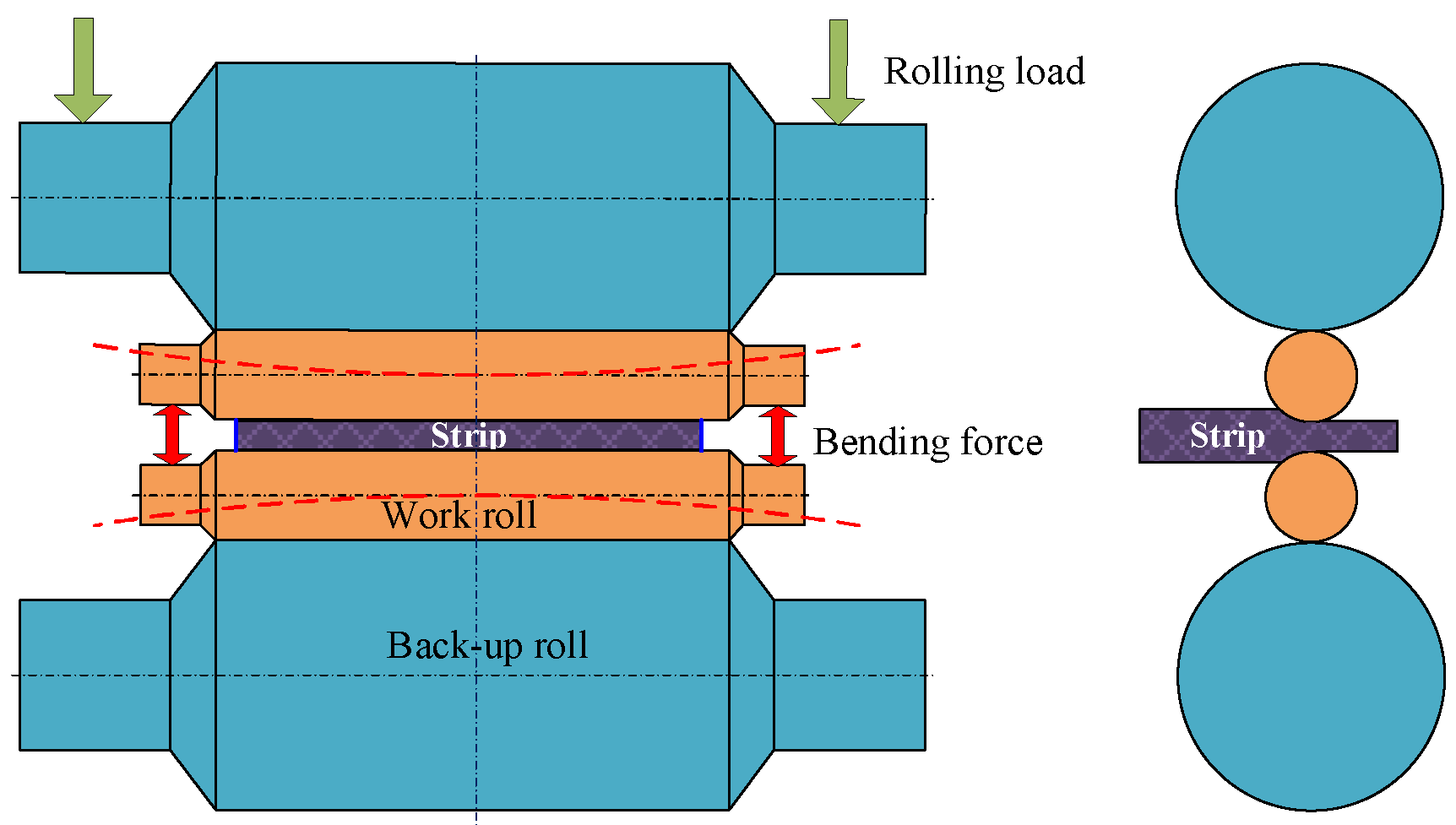
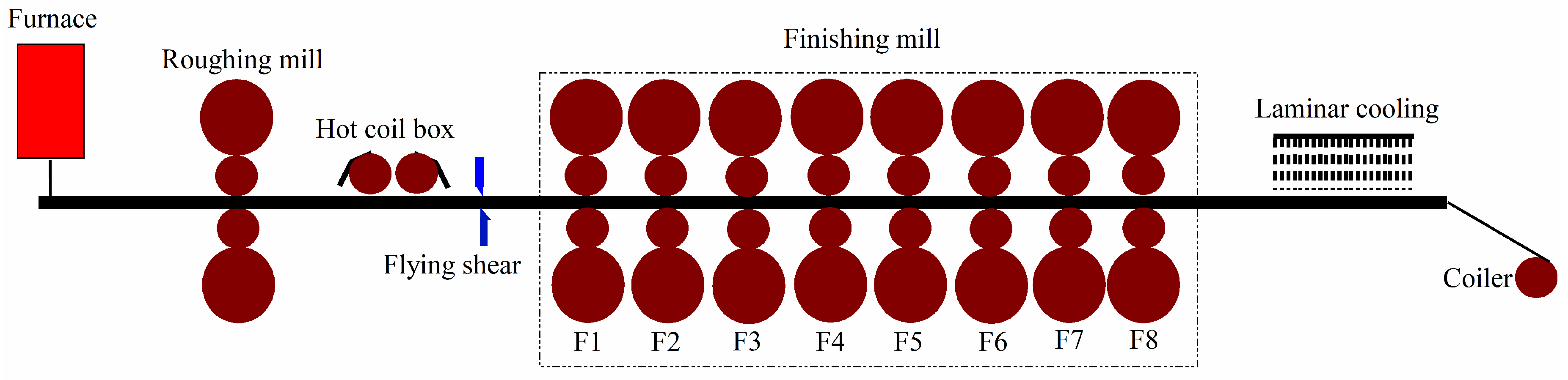
2.1. Hot Rolling Technology and Bending Force

Figure 2 shows the complete rolling process in a typical HSR process. The HSR process consists of 6 key parts: the reheating furnace, the roughing mill, the hot coil box and flying shear, the finishing mill, the laminar cooling, and the coiler. The key equipment of the production line is a finishing mill group composed of 8 groups of stands, which determines the final shape of the strip. Each group of stand consists of a pair of work rolls and a pair of backup rolls. The spacing between the stand is 5.5 m. The whole line is equipped with work roll shifting and hydraulic roll bending systems to control flatness and plate crown.

A single batch consists of a coil of rough steel, which enters the reheating furnace to be reheated to the appropriate temperature. Next, the strip passes through the roughing mill, where its thickness and width are reduced to close to the desired value. Then, the strip enters the finishing mill section, where the strip is carefully milled to the required width and thickness. The profile of the strip can be controlled by changing the bending forces between the two work rolls [25]. The strip thickness and flatness are measured in real time by an X-ray gauge at the end of the finishing stands as shown in Figure 2. Measuring the final dimensions of the strip is vital for the mill controllers. The controllers adjust mill parameters in real time with feedback from the gage to minimize strip flatness. Next, the strip is cooled by water to an appropriate final temperature. Finally, the strip is coiled and is ready for shipment.

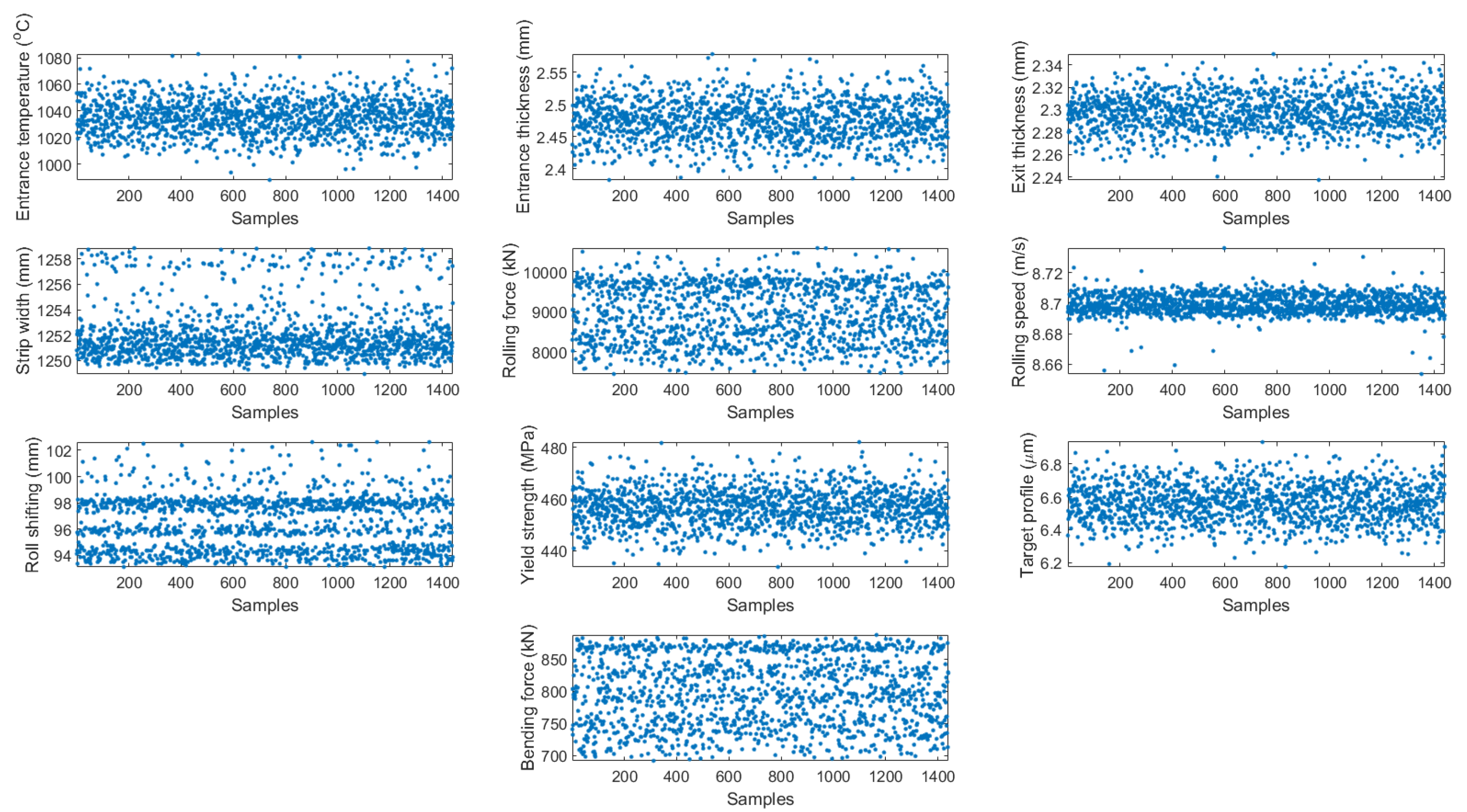
2.2. Data Collection and Analysis

In this paper, the final stand rolling data of a 1580-mm HSR process in a steel factory are collected for experiments. The purpose of models in hot rolling is to predict strip characteristics prior to rolling the strip based on information about the mill. For the proposed prediction model of bending force, the input variables are entrance temperature (°C), entrance thickness (mm), exit thickness (mm), strip width (mm), rolling force (kN), rolling speed (m/s), roll shifting (mm), yield strength (MPa), and target profile (μm). The output variable of the model is the bending force (kN). The information of the detection equipment for these parameters is shown in

Table 1. Parameter information.

Parameter	Detection Equipment	Specifications	Brand
Entrance temperature	Infrared thermometer	SYSTEM4	LAND
Exit thickness	X-ray thickness gauge	RM215	TMO
Strip width	Width gauge	ACCUBAND	KELK
Rolling force	Load Cell	Rollmax	KELK
Rolling speed	Incremental Encoder	FGH6	HUBNER
Roll shifting	Position Sensor	Tempsonics	MTS
Target profile	Profile Gauge	RM312	TMO
Bending force	Pressure Transducer	HDA3839	HYDAC

. In order to ensure the validity of the parameters, all the gauges used in this research were calibrated. The fractal dimension visualization diagram of the collected dataset is shown in Figure 3. Obviously, the input data vary considerably in different dimensions.

Table 2. Input parameters and the values.

Parameter	Unit	Mean	Range of Value
Entrance temperature	°C	1035.2	988.05~1082.8
Entrance thickness	mm	2.4750	2.3827~2.5782
Exit thickness	mm	2.2981	2.2374~2.3494
Strip width	mm	1252.0	1248.9~1258.8
Rolling force	kN	8940.4	7438.4~10,590
Rolling speed	m/s	8.6995	8.6535~8.7362
Roll shifting	mm	96.436	93.125~102.625
Yield strength	MPa	456.71	433.74~482.02
Target profile	μm	65.613	61.740~69.315

shows the data distributions for each input variables. In order to eliminate the difference between the numbers of different dimensional data, avoid prediction error increase because of the big difference between input and output data, and update the weights and biases conveniently in the modeling process. It is necessary to scale data to a small interval in a certain proportion. Normalization is required prior to data entry into the model [26]. The following formula is used to normalize the data:

$$y_i^{\prime }=\frac{y_i-y_{\min }}{y_{\max }-y_{\min }}$$

(1)

where $y_i^{\prime }$, $y_i^{}$, $y_{\min }^{}$, and $y_{\max }^{}$ are the normalized data, original data, maximal data, and minimal data, respectively.

In the present study, the K-fold cross validation method was used and 1440 pairs of measured bending force data were divided into five subsets. Four subsets were employed to train the machine learning models and the remaining one for testing the models. Furthermore, the measurement data should be processed with z-score normalization to the same scale to reduce the impact of different magnitudes and dimensions.

3. Methodology

3.1. Artificial Neural Network (ANN)

ANNs are complex computational models inspired by the human nervous system, which are capable of machine learning and pattern recognition. ANN includes a wide range of learning algorithms that have been developed in statistics and artificial intelligence. It uses analogy with biological neurons to generate general solutions to the problem. Since ANNs are nonlinear classification techniques and also composed of an interconnected group of artificial neurons, they have the ability to learn complex relationships between input and output variables [17]. ANN is the earliest prediction model applied in the rolling field, including mechanical property prediction, rolling force prediction, roughing mill temperature prediction, flatness, and crown prediction [7,8,9,10,11,12,13,14,15,16,17,18,19,20,21]. Therefore, ANN is the most widely applied model and the basic model for comparison.

3.2. Support Vector Machine (SVM)

Support Vector Machine (SVM) is a supervised learning method developed from statistical learning theory to analyze data and pattern recognition, which can be used to classify and regression data [27]. SVM as a regression technique (SVR) is a nonlinear algorithm and the basic principle is to map the data to a high-dimensional feature space using a nonlinear mapping, and then construct the regression estimation function in the high-dimensional feature space and then map back to the original space, and this nonlinear transformation is achieved by defining the appropriate kernel function. Many machine learning algorithms follow the principle of empirical error minimization, while SVR follows the principle of structural risk minimization, so it can obtain better generalization performance [28]. SVRs are prominent in research and practice, due to their use of linear optimization techniques to find optimal solutions to nonlinear predictive problems in higher-dimensional feature spaces. Therefore, it has been widely employed for regression and forecasting in the fields of agriculture, hydrology, the environment, and metallurgy [29,30,31]. This encourages us to apply an SVR to the prediction of the HSR process.

3.3. Classification and Regression Tree (CART)

Decision trees (DT) is an important algorithm for machine learning. The classification and regression tree methodology, also known as the CART was introduced in 1984 by Breiman et al. [32]. CART has low computational complexity because of its recursive computation. To predict a response, follow the decisions in the tree from the root (beginning) node down to a leaf node. The leaf node contains the response. So CART is non-parametric and can find complex relationships between input and output variables. Therefore, CART also has the advantage of discovering nonlinear structures and variables interactions in the training samples [33]. Regression tree is a data mining algorithm widely used in regression problems of biology [34], environment [35] and material processing [36]. We selected CART to prediction bending force because they are an explanatory technique, able to reveal data structure, identify important characteristics, and develop rules.

3.4. Bagging Regression Tree (BRT)

Bagging (short for bootstrap aggregating) is a simple and very powerful ensemble method. Bagging is one of the simplest techniques, which can reduce variance when combined with the base learner generation, with surprisingly good performance [37]. Bagging Regression Tree (BRT) is the application of the bootstrap procedure to RT. The basic idea underlying BRT is the recognition that part of the output error in a single regression tree is due to the specific choice of the training dataset. Therefore, if several similar datasets are created by resampling with replacement (that is, bootstrapping) and regression trees are grown without pruning and averaged, the variance component of the output error is reduced [38,39]. The BRT has been widely used in the fields of biostatistics [40], remote sensing [41], and material processing [42] due to its flexibility and interpretability to high-order nonlinear modeling. Therefore, it is reasonable to compare and evaluate BRT as one of the optional models.

3.5. Least Absolute Shrinkage and Selection Operator (LASSO)

LASSO stands for Least Absolute Shrinkage and Selection Operator [43]. The idea behind the LASSO algorithm is to achieve a minimization of the residual sum of squares while regularizing the sum of the absolute value of the coefficients being less than a given constant. LASSO technique has been successfully developed in recent years, combining shrinkage and highly correlated variables. LASSO regression is characterized by variable selection and regularization while fitting the generalized linear model. Regularization is to control the complexity of the model through a series of parameters so as to avoid over fitting. LASSO has been widely used in temperature prediction [44], the wavelength analysis [45], and streamflow prediction [46]. In view of its wide application in industry, LASSO is also taken as one of the research models in this paper.

3.6. Gaussian Process Regression (GPR)

Gaussian Process Regression (GPR) is a new machine learning regression method developed in recent years, and it is also a non-parametric model algorithm based on Bayesian network. The GPR algorithm can adaptively determine the number of model parameters according to the information of the training samples, and add the prior knowledge of the existing objects in the modeling process, and then combine the actual experimental data to obtain the posterior Gauss process model [47]. When GPR is applied to practical problems, GPR can give a confidence interval while outputting the mean value, making the validity of the prediction result continuously enhanced. In addition, because the GPR can quantitatively model Gaussian noise, it has excellent prediction accuracy [48,49]. Because of its good predictive ability, GPR has been widely used in data-driven modeling of various problems in industry [50,51,52,53], so GPR has also become an optional scheme in this paper.

3.7. Model Information

All models were implemented in Matlab (Version 2015b, MathWorks, Natick, MA, USA) under a computer with a hardware configuration of Intel Core i7-7500U CPU 2.7 GHz, and 8 GB of RAM. CART, BRT, LASSO, and GPR were carried out with treefit, fitensemble, lasso, and fitrgp functions, respectively. These four functions are included in Matlab’s Statistics and Machine Learning Toolbox. The parameters of these models were automatically optimized by Matlab function according to the training dataset. For SVR, the parameter C (trade-off parameter between the minimization of errors and smoothness of the solution), and the parameter σ (the width of the RBF kernel function) are needed to determine the process of model establishment. In order to reveal the effect of C and σ on prediction results in training dataset. Ten logarithmically, equally spaced points were generated between 1 and 1000 for C. Twenty logarithmically, equally spaced points were generated between 10 and 1000 for σ. The optimized C and σ were determined to be 100 and 69.5, respectively. For ANN, the transfer function of hidden layer and output layer are “tansig” and “purelin”, respectively. The “tainlm” (Levenberg-Marquardt) was chosen as the optimal learning algorithm. In this paper, the performance of neural networks with 2–30 neurons was investigated considering the single hidden layer. The number of neurons in the network hidden layer is determined to be 6, and the ANN has the best performance.

3.8. Comparison of Model and Statistical Error Analysis

The accuracy and performance of the studied models for bending force prediction were evaluated and compared using three commonly used statistical metrics, which were root mean square error (RMSE, Equation (2)), mean absolute error (MAE, Equation (3)), and coefficient of determination (R², Equation (4)). The mathematical equations of the statistical indicators are described below.

$$\mathrm{RMSE}=\sqrt{\frac{{\displaystyle {\sum }_{i=1}^N{(y_i-y_i^{*})}^2}}{N}}\mathrm{a}=1$$

(2)

$$\mathrm{MAE}=\frac{1}{N}{\displaystyle {\sum }_{i=1}^N\left|y_i-y_i^{*}\right|}$$

(3)

$${\mathrm{R}}^2=1-\frac{{\displaystyle {\sum }_{i=1}^N{(y_i-y^{*})}^2}}{{\displaystyle {\sum }_{i=1}^N{(y_i-\overline{y})}^2}}$$

(4)

where $y_i\mathrm{and}{y}_i^{*}$ are the measured values and predictive values respectively, N is the total number of predicted data. Higher values of R² are preferred, i.e., closer to 1 means better model performance and regression line fits the data well. On the contrary, the lower the RMSE and MAE values are, the better the model performs.

4. Results

4.1. Prediction Accuracy of Various Models

Table 3. Accuracy statistical results of the six machine learning models performing 30 trials in training and testing dataset.

Model		Training Dataset			Testing Dataset
		RMSE (kN)	MAE (kN)	R2	RMSE (kN)	MAE (kN)	R2
ANN	Max	10.3392	8.0444	0.9678	11.1894	8.6467	0.9621
	Min	9.3885	7.2853	0.9611	10.1867	7.8557	0.9543
	Mean	9.7603	7.6325	0.9653	10.5676	8.2064	0.9590
SVM	Max	13.0896	10.3777	0.9400	13.4531	10.7890	0.9371
	Min	12.8499	9.9659	0.9378	13.1528	10.3986	0.9328
	Mean	12.9733	10.1730	0.9389	13.2755	10.5367	0.9356
CART	Max	9.1048	6.8205	0.9749	10.5625	7.8368	0.9640
	Min	8.3138	6.3089	0.9699	9.9445	7.2870	0.9591
	Mean	8.7054	6.5526	0.9724	10.2547	7.5449	0.9615
BRT	Max	6.1908	4.7867	0.9865	9.7559	7.6485	0.9674
	Min	6.1018	4.7222	0.9861	9.4643	7.4094	0.9653
	Mean	6.1552	4.7561	0.9862	9.6441	7.5587	0.9660
LASSO	Max	13.5908	11.2526	0.9345	14.5408	11.9976	0.9330
	Min	13.4307	11.0978	0.9329	13.5506	11.1993	0.9222
	Mean	13.5261	11.1914	0.9336	14.0047	11.5624	0.9283
GPR	Max	7.4269	5.7891	0.9805	8.6418	6.6802	0.9745
	Min	7.3335	5.7243	0.9800	8.3605	6.5054	0.9726
	Mean	7.3887	5.7580	0.9802	8.5121	6.6137	0.9735

Note: Abbreviations: root mean square error, RMSE; mean absolute error, MAE; coefficient of determination, R²; Artificial Neural Network, ANN; Support Vector Machine, SVR; Classification and Regression Tree, CART; Bagging Regression Tree, BRT; Least Absolute Shrinkage and Selection operator, LASSO; Gaussian Process Regression, GPR.

shows the results of the ANN, SVM, CART, BRT, LASSO, and GPR models performing 30 trials in training and testing dataset. It can be seen that the predicted bending force varies considerably depending on the model selection. In training dataset, no matter which evaluation metrics are used, BRT shows the best prediction performance with the highest R² and lowest RMSE and MAE. In testing dataset, GPR shows the best prediction performance with the highest R² and lowest RMSE and MAE. The prediction performance of BRT follows that of GPR. On the contrary, LASSO has the worst prediction accuracy not only in the training dataset but also in the testing dataset.

Figure 4 shows the accuracy ranking results of the six models in training and testing dataset. The prediction accuracy value of the model can be read out from the ordinate, and the ranking results of these models are showed with numbers above the color bars. As can be seen from Figure 4, first of all, the accuracy ranking results show slight difference in training and testing dataset. In training dataset, the accuracy ranking results is consistent with the three evaluation metrics, and the rank order is: BRT, GPR, CART, ANN, SVM, LASSO. However, the accuracy ranking result changes slightly in testing dataset. In addition, with different accuracy evaluation metrics, the accuracy ranking results are also different. The accuracy rank with the metrics of RMSE and R² in descending order is: GPR, BRT, CART, ANN, SVM, LASSO; and that of MAE in descending order is: GPR, CART, BRT, ANN, SVM, LASSO. Based on the comprehensive performance of the two datasets, it can be considered that GPR model shows the best prediction accuracy and LASSO model has the worst prediction accuracy.

The scatter plot of the bending force values measured by the factory and the values predicted by the six machine learning models in training and testing dataset are presented in Figure 5. Scattered points of different colors in the figure represent the predicted values by different models. In training and testing dataset, the predicted values of BRT and GPR models are closely distributed on both sides of the straight line y = x. The results show that the predicted bending force of the two models have a better correlation with the measured bending force value, and the two models are superior to the other four models for bending force prediction. On the contrary, LASSO has the worst prediction accuracy with the most scattered predicted value around the straight line y = x, indicating that the predicted values are much different from the measured values. The maximum error of all other data points predicted by the six models is within 10%. Therefore, these six models have achieved good prediction performance.

Figure 6 shows the measured bending force and predicted bending force by the six models in training and testing dataset, and also shows prediction errors below. It clearly shows that the BRT has the best prediction performance in training dataset, the maximum positive error is 23.60 kN and the maximum negative error is −25.28 kN. In testing dataset, GPR has the best prediction performance with the maximum positive error as 31.84 kN and the maximum negative error as −26.50 kN. The errors of BRT and GPR are more concentrated in the range of 0 kN, which means that the number of samples with large error values is smaller. On the contrary, the LASSO performs worst in the six models of two datasets. In training dataset, the maximum positive error is 41.07 kN and the maximum negative error is −44.56 kN. In testing datasets, the maximum positive error is 42.99 kN and the maximum negative error is −27.04 kN.

Figure 7 shows the histograms and distribution curves of the errors. All the error distribution curves have a bell shape of normal distribution, which indicates that the prediction errors of all models are normal distribution. Whether in training or in testing datasets, GPR, BRT, and CART models perform relatively well, and their normal distribution curves are higher and narrower, which indicate that more prediction values with smaller errors are obtained. In addition, it is also found that the dataset centers (the highest point of normal distribution curve) of most models are close to the zero point of errors. The dataset center represents the average value of errors, indicating that the probabilities of positive error and negative error are almost equal. However, the normal distribution curve of LASSO shifts to right obviously in testing dataset, which indicates that the positive error of LASSO model is much more than the negative error and the predicted values are higher.

4.2. Stability of Various Models

The prediction accuracy results show that the prediction accuracy in testing dataset of all models is lower than that in the training dataset. In addition, in training dataset, the prediction accuracy of BRT model is better than the GPR. However, in testing dataset, the prediction accuracy of GPR model is better than the BRT (showed in Figure 4). The difference of prediction accuracy between in training and testing dataset can be regarded as the stability of the model. The stability of machine learning model is also an important factor affecting the prediction performance, which should be taken into account when evaluating the reliability of predicted result. The stability of the machine learning model is the relative change percentage of the evaluation metrics (including RMSE, MAE, and R²) of the model in training and testing datasets [31]. The smaller the relative change percentage, the higher the stability of the model. The relative change percentage of evaluation metrics under the two datasets can be described by δ_i,N and calculated by the following formula:

$${\delta }_{\mathrm{i},\mathrm{N}}=\left|\frac{{\delta }_{i,test}-{\delta }_{i,train}}{{\delta }_{i,train}}\right|\times 100\%$$

(5)

where i represent the evaluation metrics (RMSE, MAE, or R²) and N represent the one of the six models.

Figure 8 shows the δ_i,N from three evaluation metrics of the six models performing 30 trials. It shows that the stability rankings of ANN, SVR, CART, BRT, LASSO, and GPR models are slightly different with different evaluation metrics. With the evaluation metrics of RMSE and R², SVR shows the most stable performance with the lowest δ_i,N values of 2.33% and 0.35%, respectively. LASSO shows the most stable performance with the lowest δ_i,N values of 2.33% in the evaluation metrics of MAE. However, no matter which evaluation metrics is used, the BRT shows the most unstable performance with the highest δ_i,N. The δ_i,N are 56.68%, 58.93%, and 2.05% calculated by RMSE, MAE, and R², respectively. This unstable performance reveals that when new input data is used, it will lead to a significant reduction in prediction accuracy. This is because the BRT model has a large number of hyper-parameters, which need to be carefully optimized for model application [31].

The distribution of the three evaluation metrics obtained from six machine learning models performing 30 trials in training and testing dataset are illustrated in Figure 9 using a boxplot. It represents the degree of spread for the prediction accuracy with its respective quartile. In training dataset, the suspected outliers of the prediction accuracy only appear in ANN and CART models. In testing dataset, suspected outliers appear in ANN, SVM, CART, and BRT models. At the same time, it is found that the quartile distance of testing dataset is increasing compared with that in training dataset, which indicates that the degree of dispersion of prediction accuracy became larger. Although Figure 8 shows that both SVM and LASSO models have the most stable performance. However, the variation of the quartile distance of the LASSO model is most obvious in the two datasets. Considering comprehensively, it can be considered that SVM is the most stable model.

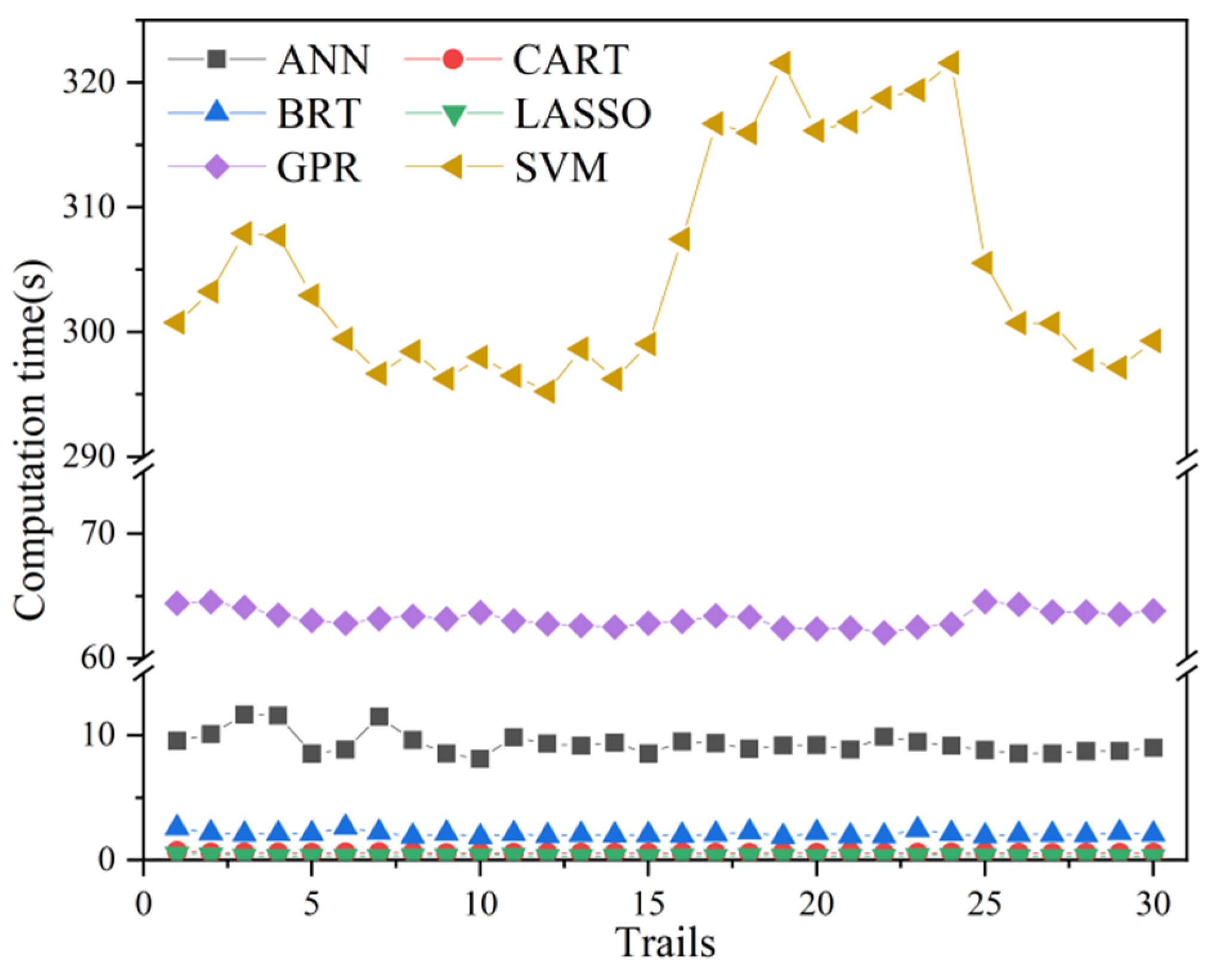
4.3. Computational Costs of Various Models

Table 4. Comparison of computational costs (time used for computation) of the six machine learning models.

Model	Computational Cost (s)
	Max	Min	Mean
ANN	11.66	8.12	9.35
SVM	321.59	295.24	305.09
CART	0.71	0.56	0.59
BRT	2.64	1.87	2.11
LASSO	0.51	0.31	0.35
GPR	64.55	62.06	63.25

Note: The lowest computational cost among all models are marked in bold.

and Figure 10 shows the computational cost (time used for computation) of the six machine learning models. The CART and LASSO show the lowest computational costs of 0.59 s and 0.35 s, respectively. BRT and ANN also show smaller computational costs of 2.11 s and 9.35 s, respectively. Compared with the above four models, the computational cost of GPR increases to 63.25 s. Furthermore, the computational cost of SVM reaches the maximum value, which is 305.09 s.

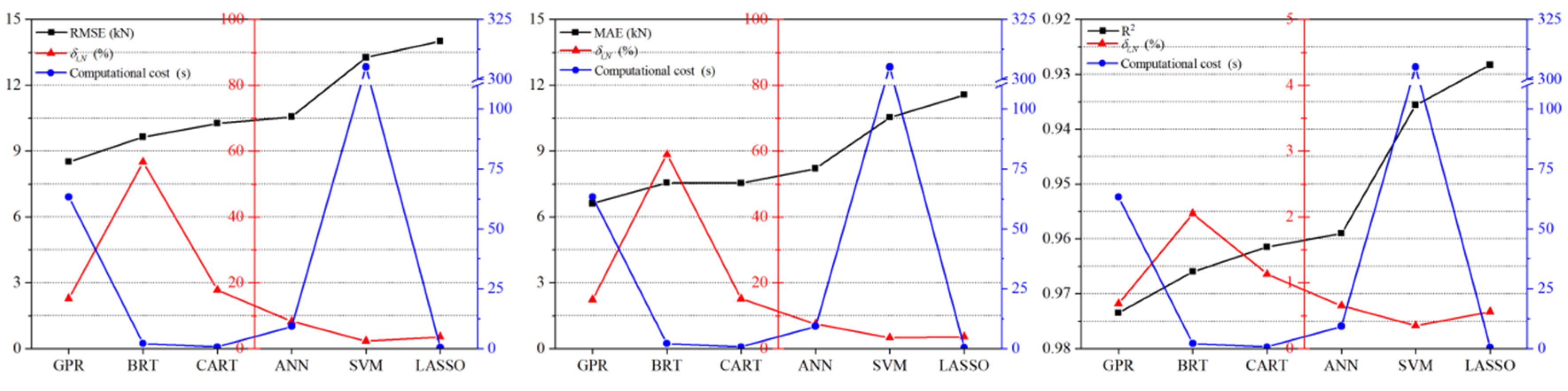
4.4. Comprehensive Evaluation of Various Models

Based on the above results, six machine learning models comprehensively evaluated from prediction accuracy, stability, and computational cost, and the results are shown in Figure 11. It must be pointed out that the prediction accuracy here is in testing dataset. Figure 11 shows that GPR provides the best combination of prediction accuracy, stability, and computational cost. The prediction accuracy of BRT, CART, and ANN models is slightly worse than that of GPR. For the three models, the prediction accuracy and computational cost of them are not much different, but BRT has the worst stability. In addition, SVM does not perform well in terms of prediction accuracy and computational cost. LASSO has good stability and computational cost, but the prediction accuracy is the worst.

5. Discussion

With the development of technology, today, in the production process of a series of steel, the equipment will maintain a stable operation state, so the rolling process is also carried out stably. Therefore, for specific strip specification, most rolling processes will obtain relatively stable datasets without large variability. Then, the key technology of rolling parameter prediction is how to improve the prediction accuracy. The stable data can better reflect the normal rolling process. The purpose of this paper is to discuss the comparison results of prediction accuracy when different models are applied to bending force prediction. Therefore, in order to reflect the most essential characteristics of the model and obtain a fair comparison result, the machine learning models used in this paper were not over optimized by combining with other intelligent optimization algorithms (such as Genetic Algorithm (GA), Particle Swarm Optimization (PSO), etc.). We believe that this paper can be used as a reference and basis for other similar prediction applications and research to select machine learning models, and it is more practical to select basic original models and parameters.

6. Conclusions

In this paper, we applied six machine learning models, including ANN, SVR, CART, BRT, LASSO, and GPR, to predict the bending force in the HSR process. A comparative experiment was carried out based on real-life dataset, and the prediction performance of the six models was analyzed from prediction accuracy, stability, and computational cost. All the gauges used in this research were calibrated to ensure the validity of the data and reliability of the results. The prediction performance of the six models was assessed using three evaluation metrics of RMSE, MAE, and R².

(1)

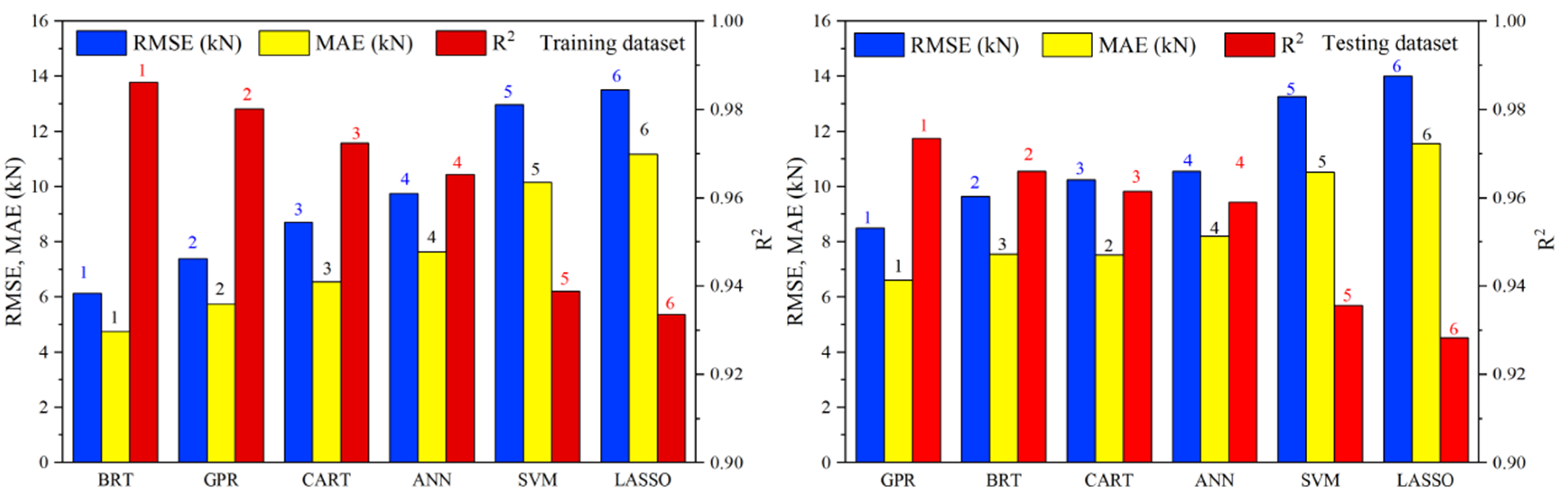
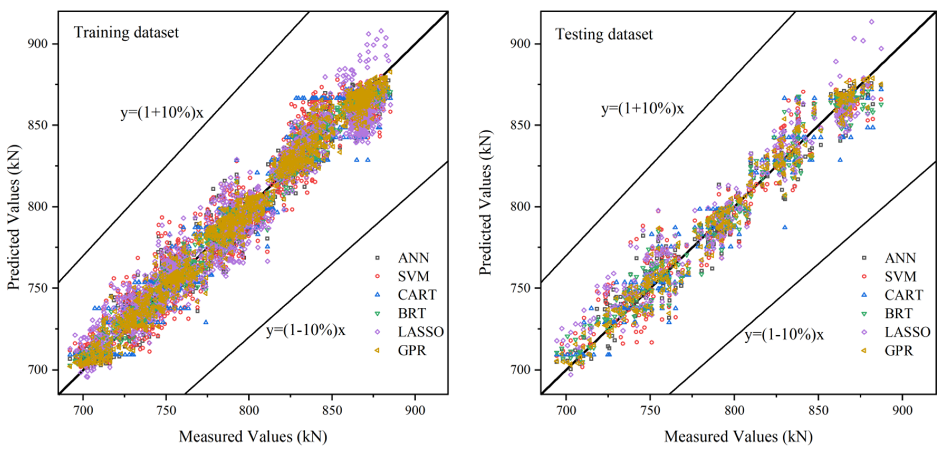
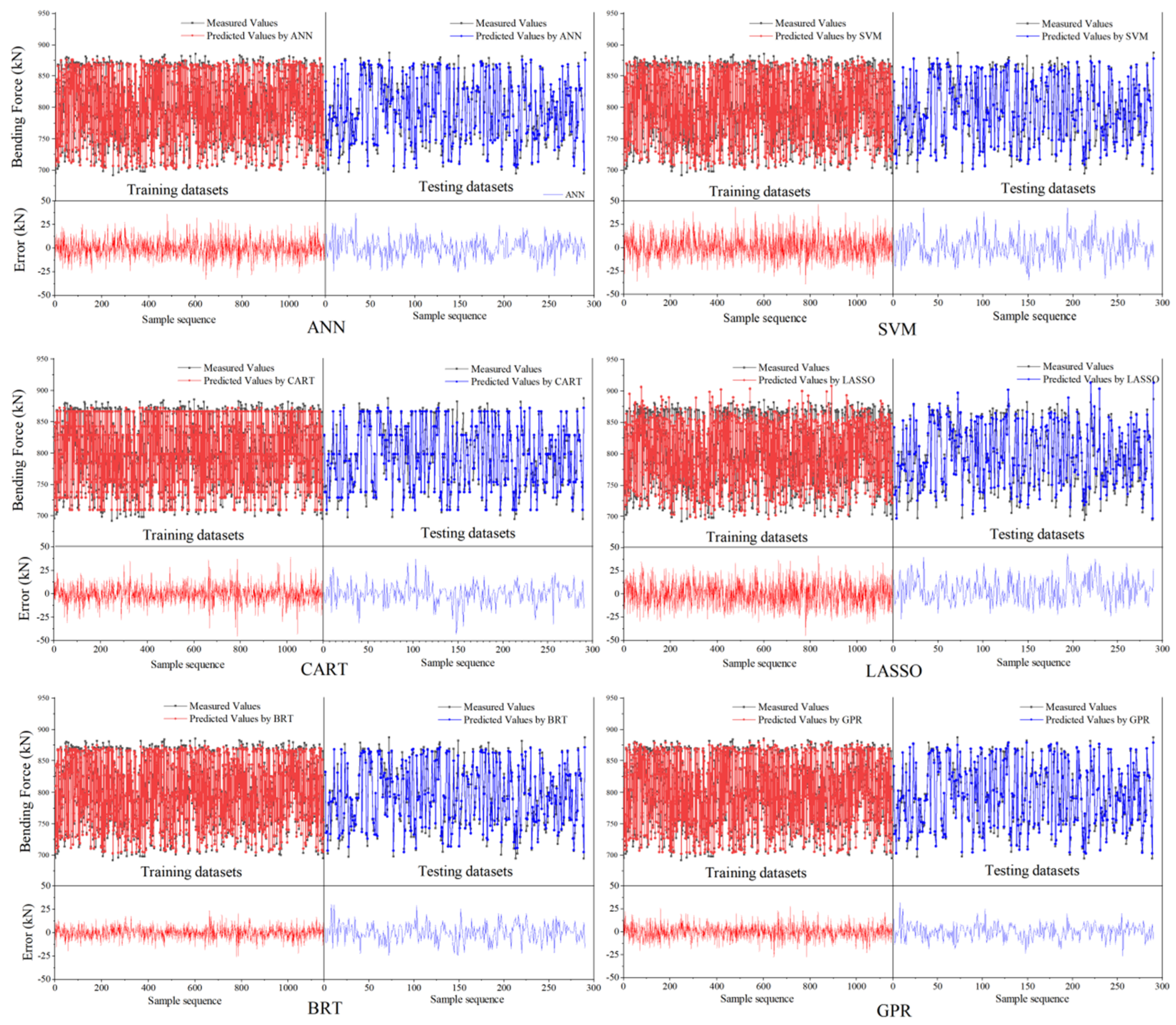
The comparison results of prediction accuracy show that the accuracy ranking results in testing dataset are slightly different under the three evaluation metrics. However, considering that GPR performs best, followed by BRT, CART, ANN, SVM, and LASSO respectively. The bending force measured by experiment is 690~890 kN, while the prediction error of GPR is only 8.51 kN (RMSE) and 6.61 kN (MAE).

(2)

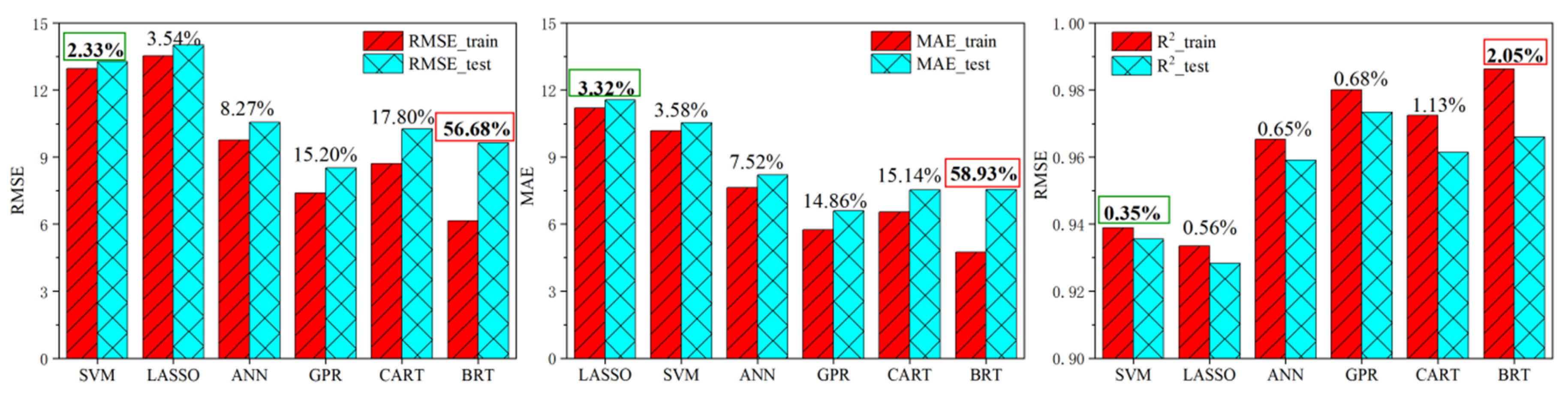
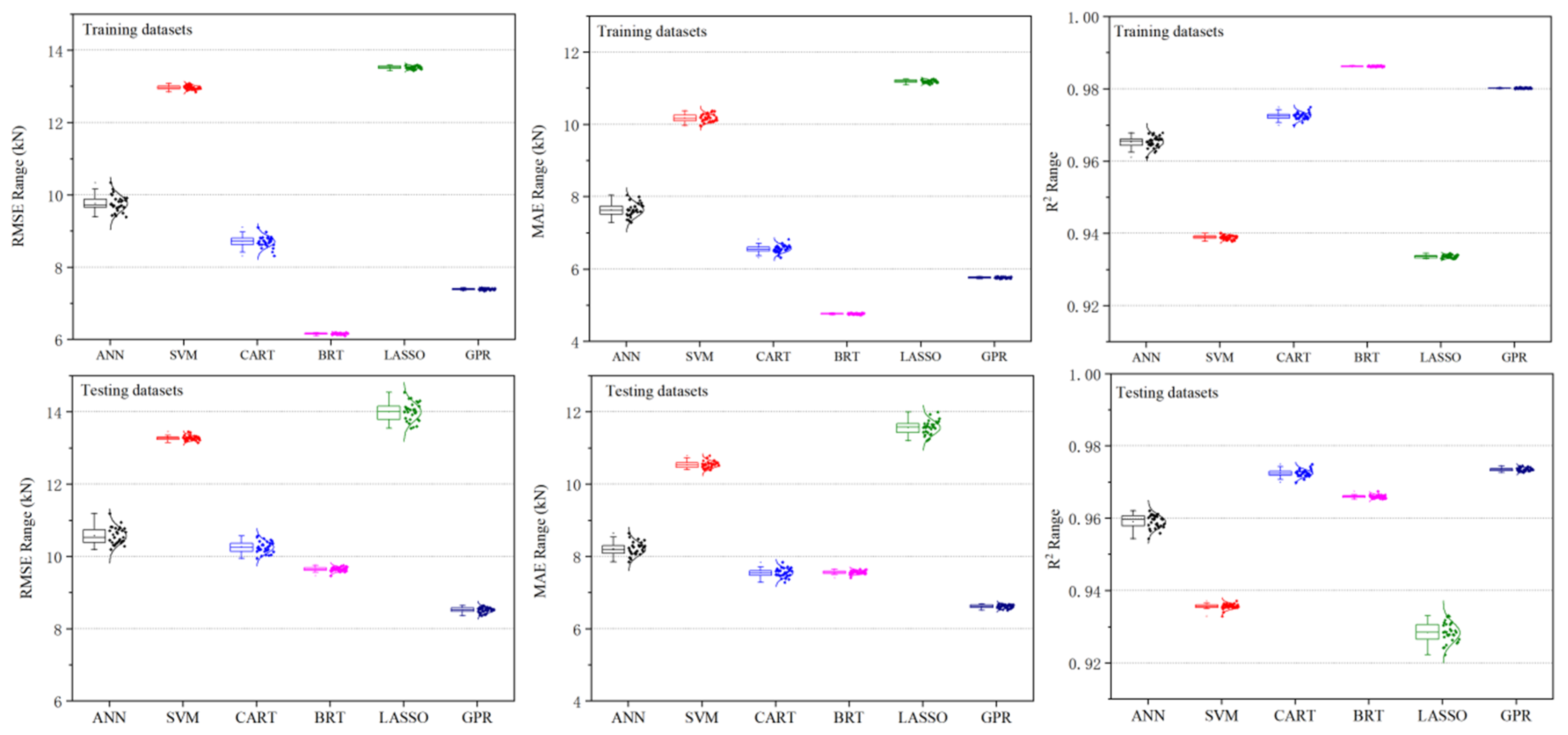
The ranking results of stability show inconsistency in the three evaluation metrics. However, considering comprehensively, SVM shows the most stable performance with the γ of 2.33% (RMSE), 0.32% (MAE) and 0.35% (R²). The stability decreases in the order of LASSO, ANN, GPR, CART, and BRT. BRT shows the most unstable performance with the γ of 56.68% (RMSE), 58.93% (MAE), and 2.05% (R²).

(3)

The computational cost of the six models presents three levels. The computational costs of LASSO, CART, BRT, and ANN are increasing gradually, but they are all within ten seconds. The computational cost of GPR model is slightly higher, at about 63 s. However, the computational cost of SVM has reached more than 300 s.

(4)

Comprehensively considering the prediction accuracy, stability, and computational cost of the six models, GPR can be considered the most promising machine learning model for predicting bending force. The prediction accuracy and stability of CART and ANN is slightly lower than GPR, but the computational cost is relatively small, so it can also be used as an alternative. In addition, BRT also shows the better combination of prediction accuracy and computational cost, but the stability of BRT is the worst among the six models. SVM not only performs poorly in prediction accuracy, but also has the greatest computational cost. While LASSO has good stability and small computational cost, but it also has the worst prediction accuracy.

References

1. Takahashi, R.R. State of the art in hot rolling process control. Control Eng. Pract. 2001, 9, 987–993. [Google Scholar] [CrossRef]
2. Zhu, H.T.; Jiang, Z.Y.; Tieu, A.K.; Wang, G.D. A fuzzy algorithm for flatness control in hot strip mill. J. Mater. Process. Technol. 2003, 140, 123–128. [Google Scholar] [CrossRef]
3. Wang, Q.L.; Sun, J.; Liu, Y.M.; Wang, P.F.; Zhang, D.H. Analysis of symmetrical flatness actuator efficiencies for UCM cold rolling mill by 3D elastic-plastic FEM. Int. J. Adv. Manuf. Technol. 2017, 92, 1371–1389. [Google Scholar] [CrossRef]
4. Jia, C.Y.; Shan, X.Y.; Cui, Y.C.; Bai, T.; Cui, F.J. Modeling and Simulation of Hydraulic Roll Bending System Based on CMAC Neural Network and PID Coupling Control Strategy. J. Iron Steel Res. Int. 2013, 20, 17–22. [Google Scholar] [CrossRef]
5. Zhang, S.H.; Deng, L.; Zhang, Q.Y.; Li, Q.H.; Hou, J.X. Modeling of rolling force of ultra-heavy plate considering the influence of deformation penetration coefficient. Int. J. Mech. Sci. 2019, 159, 373–381. [Google Scholar] [CrossRef]
6. Zhang, S.H.; Song, B.N.; Gao, S.W.; Guan, M.; Zhao, D.W. Upper bound analysis of a shape-dependent criterion for closing central rectangular defects during hot rolling. Appl. Math. Model. 2018, 55, 674–684. [Google Scholar] [CrossRef]
7. Zhang, W.; Wang, Y.; Sum, M. Modeling and Simulation of Electric-Hydraulic Control System for Bending Roll System. In Proceedings of the 2008 IEEE Conference on Robotics, Automation and Mechatronics (RAM), Chengdu, China, 21–24 September 2008; pp. 1–4. [Google Scholar] [CrossRef]
8. Sterjovski, Z.; Nolan, D.; Carpenter, K.R.; Dunne, D.P.; Norrish, J. Artificial neural networks for modeling the mechanical properties of steels in various applications. J. Mater. Process. Technol. 2015, 170, 536–544. [Google Scholar] [CrossRef]
9. Wang, P.; Huang, Z.Y.; Zhang, M.Y.; Zhao, X.W. Mechanical Property Prediction of Strip Model Based on PSO-BP Neural Network. J. Iron Steel Res. Int. 2008, 15, 87–91. [Google Scholar] [CrossRef]
10. Ozerdem, M.S.; Kolukisa, S. Artificial Neural Network approach to predict mechanical properties of hot rolled, nonresulfurized, AISI 10xx series carbon steel bars. J. Mater. Process. Technol. 2008, 199, 437–439. [Google Scholar] [CrossRef]
11. Bagheripoor, M.; Bisadi, H. Application of artificial neural networks for the prediction of roll force and roll torque in hot strip rolling process. Appl. Math. Model. 2013, 37, 4593–4607. [Google Scholar] [CrossRef]
12. Lee, D.; Lee, Y. Application of neural-network for improving accuracy of roll-force model in hot-rolling mill. Control Eng. Pract. 2002, 10, 473–478. [Google Scholar] [CrossRef]
13. Mahmoodkhani, Y.; Wells, M.A.; Song, G. Prediction of roll force in skin pass rolling using numerical and artificial neural network methods. Ironmak. Steelmak. 2017, 44, 281–286. [Google Scholar] [CrossRef]
14. Yang, Y.Y.; Linkens, D.A.; Talamantes-Silva, J.; Howard, I.C. Roll force and torque prediction using neural network and finite element modelling. ISIJ Int. 2003, 43, 1957–1966. [Google Scholar] [CrossRef]
15. Laurinen, P.; Röning, J. An adaptive neural network model for predicting the post roughing mill temperature of steel slabs in the reheating furnace. J. Mater. Process. Technol. 2005, 168, 423–430. [Google Scholar] [CrossRef]
16. John, S.; Sikdar, S.; Swamy, P.K.; Das, S.; Maity, B. Hybrid neural-GA model to predict and minimise flatness value of hot rolled strips. J. Mater. Process. Technol. 2008, 195, 314–320. [Google Scholar] [CrossRef]
17. Deng, J.F.; Sun, J.; Peng, W.; Hu, Y.H.; Zhang, D.H. Application of neural networks for predicting hot-rolled strip crown. Appl. Soft Comput. 2019, 78, 119–131. [Google Scholar] [CrossRef]
18. Kim, D.H.; Lee, Y.; Kim, B.M. Application of ANN for the dimensional accuracy of workpiece in hot rod rolling process. J. Mater. Process. Technol. 2002, 130–131, 214–218. [Google Scholar] [CrossRef]
19. Alaei, H.; Salimi, M.; Nourani, A. Online prediction of work roll thermal expansion in a hot rolling process by a neural network. Int. J. Adv. Manuf. Technol. 2016, 85, 1769–1777. [Google Scholar] [CrossRef]
20. Sikdar, S.; Kumari, S. Neural network model of the profile of hot-rolled strip. Int. J. Adv. Manuf. Technol. 2009, 42, 450–462. [Google Scholar] [CrossRef]
21. Wang, Z.H.; Gong, D.Y.; Li, X.; Li, G.; Zhang, D. Prediction of bending force in the hot strip rolling process using artificial neural network and genetic algorithm (ANN-GA). Int. J. Adv. Manuf. Technol. 2017, 93, 3325–3338. [Google Scholar] [CrossRef]
22. Laha, D.; Ren, Y.; Suganthan, P.N. Modeling of steelmaking process with effective machine learning techniques. Expert Syst. Appl. 2015, 42, 4687–4696. [Google Scholar] [CrossRef]
23. Hu, Z.Y.; Wei, Z.H.; Sun, H.; Yang, J.M.; Wei, L.X. Optimization of Metal Rolling Control Using Soft Computing Approaches: A Review. Arch. Comput. Methods Eng. 2019, 11, 1–17. [Google Scholar] [CrossRef]
24. Shardt, Y.A.W.; Mehrkanoon, S.; Zhang, K.; Yang, X.; Suykens, J.; Ding, S.X.; Peng, K. Modelling the strip thickness in hot steel rolling mills using least-squares support vector machines. Can. J. Chem. Eng. 2018, 96, 171–178. [Google Scholar] [CrossRef]
25. Peng, K.X.; Zhong, H.; Zhao, L.; Xue, K.; Ji, Y.D. Strip shape modeling and its setup strategy in hot strip mill process. Int. J. Adv. Manuf. Technol. 2014, 72, 589–605. [Google Scholar] [CrossRef]
26. Leaman, R.; Dogan, R.I.; Lu, Z.Y. Dnorm: Disease name normalization with pairwise learning to rank. Bioinformatics 2013, 29, 2909–2917. [Google Scholar] [CrossRef] [Green Version]
27. Cortes, C.; Vapnik, V. Support-vector networks. Mach. Learn. 1995, 20, 273–297. [Google Scholar] [CrossRef]
28. Smola, A.J.; Schölkopf, B. A Tutorial on Support Vector Regression. Stat. Comput. 2004, 14, 199–222. [Google Scholar] [CrossRef] [Green Version]
29. Shrestha, N.K.; Shukla, S. Support vector machine based modeling of evapotranspiration using hydro-climatic variables in a sub-tropical environment. Agric. Forest Meteorol. 2015, 200, 172–184. [Google Scholar] [CrossRef]
30. Ghorbani, M.A.; Shamshirband, S.; Haghi, D.Z.; Azani, A.; Bonakdari, H.; Ebtehaj, I. Application of firefly algorithm-based support vector machines for prediction of field capacity and permanent wilting point. Soil Tillage Res. 2017, 172, 32–38. [Google Scholar] [CrossRef]
31. Fan, J.; Yue, W.; Wu, L.; Zhang, F.; Cai, H.; Wang, X.; Lu, X.; Xiang, Y. Evaluation of SVM, ELM and four tree-based ensemble models for predicting daily reference evapotranspiration using limited meteorological data in different climates of China. Agric. Forest Meteorol. 2018, 263, 225–241. [Google Scholar] [CrossRef]
32. Gordon, A.D. Classification and Regression Trees. In Biometrics; Breiman, L., Friedman, J.H., ROlshen, A., Stone, C.J., Eds.; International Biometric Society: Washington, DC, USA, 1984; Volume 40, p. 874. [Google Scholar] [CrossRef] [Green Version]
33. Brezigar-Masten, A.; Masten, I. CART-based selection of bankruptcy predictors for the logic model. Expert Syst. Appl. 2012, 39, 10153–10159. [Google Scholar] [CrossRef]
34. Vondra, M.; Touš, M.; Teng, S.Y. Digestate evaporation treatment in biogas plants: A techno-economic assessment by Monte Carlo, neural networks and decision trees. J. Clean. Prod. 2019, 238, 117870. [Google Scholar] [CrossRef] [Green Version]
35. Günay, M.E.; Türker, L.; Tapan, N.A. Decision tree analysis for efficient CO2 utilization in electrochemical systems. J. CO2 Util. 2018, 28, 83–95. [Google Scholar] [CrossRef]
36. Madhusudana, C.K.; Kumar, H.; Narendranath, S. Fault Diagnosis of Face Milling Tool using Decision Tree and Sound Signal. Mater. Today Proc. 2018, 5, 12035–12044. [Google Scholar] [CrossRef]
37. Wang, G.; Hao, J.; Mab, J.; Jiang, H. A comparative assessment of ensemble learning for credit scoring. Exp. Syst. Appl. 2011, 38, 223–230. [Google Scholar] [CrossRef]
38. Breiman, L. Bagging predictors. Mach. Learn. 1996, 24, 123–140. [Google Scholar] [CrossRef] [Green Version]
39. Bühlmann, P.; Yu, B. Analyzing Bagging. Ann. Stat. 2002, 30, 927–961. [Google Scholar] [CrossRef]
40. Hothorn, T.; Lausen, B.; Benner, A.; Radespiel-Troger, M. Bagging survival trees. Stat. Med. 2004, 23, 77–91. [Google Scholar] [CrossRef]
41. Chan, C.W.; Huang, C.; Defries, R. Enhanced algorithm performance for land cover classification from remotely sensed data using bagging and boosting. IEEE Trans. Geosci. Remote 2001, 39, 693–695. [Google Scholar] [CrossRef]
42. Wang, X.J.; Yuan, P.; Mao, Z.Z.; You, M.S. Molten steel temperature prediction model based on bootstrap Feature Subsets Ensemble Regression Trees. Knowl.-Based Syst. 2016, 1011, 48–59. [Google Scholar] [CrossRef]
43. Tibshirani, R. Regression shrinkage and selection via the lasso. J. R. Stat. Soc. B Met. 1996, 58, 267–288. [Google Scholar] [CrossRef]
44. Spencer, B.; Alfandi, O.; Al-Obeidat, F. A Refinement of Lasso Regression Applied to Temperature Forecasting. Procedia Comput. Sci. 2018, 130, 728–735. [Google Scholar] [CrossRef]
45. Zhang, R.Q.; Zhang, F.Y.; Chen, W.C.; Yao, H.M.; Guo, J.; Wu, S.C.; Wu, T.; Du, Y.P. A new strategy of least absolute shrinkage and selection operator coupled with sampling error profile analysis for wavelength selection. Chemometr. Intell. Lab. 2018, 17515, 47–54. [Google Scholar] [CrossRef]
46. Chu, H.B.; Wei, J.H.; Wu, W.Y. Streamflow prediction using LASSO-FCM-DBN approach based on hydro-meteorological condition classification. J. Hydrol. 2020, 580, 124253. [Google Scholar] [CrossRef]
47. Sniekers, S.; Vaart, A.V.D. Adaptive Bayesian credible sets in regression with a Gaussian process prior. Statistics 2015, 9, 2475–2527. [Google Scholar] [CrossRef]
48. Liu, H.T.; Cai, J.F.; Ong, Y.S.; Wang, Y. Understanding and comparing scalable Gaussian process regression for big data. Knowl.-Based Syst. 2019, 164, 324–335. [Google Scholar] [CrossRef] [Green Version]
49. Kong, D.; Chen, Y.; Li, N. Gaussian process regression for tool wear prediction. Mech. Syst. Signal Pr. 2018, 104, 556–574. [Google Scholar] [CrossRef]
50. Wang, B.; Chen, T. Gaussian process regression with multiple response variables. Chemometr. Intell. Lab. 2015, 142, 159–165. [Google Scholar] [CrossRef] [Green Version]
51. Zhang, C.; Wei, H.; Zhao, X.; Liu, T.; Zhang, K. A Gaussian process regression based hybrid approach for short-term wind speed prediction. Energy Convers. Manag. 2016, 126, 1084–1092. [Google Scholar] [CrossRef]
52. Aye, S.A.; Heyns, P.S. An integrated Gaussian process regression for prediction of remaining useful life of slow speed bearings based on acoustic emission. Mech. Syst. Signal Pr. 2017, 84, 485–498. [Google Scholar] [CrossRef]
53. Liu, Y.Q.; Pan, Y.P.; Huang, D.P.; Wang, Q.L. Fault prognosis of filamentous sludge bulking using an enhanced multi-output gaussian processes regression. Control Eng. Pract. 2017, 62, 46–54. [Google Scholar] [CrossRef]
Figure 1. The schematic diagram of hydraulic roll bending technique.
Metals 10 00685 g001
Figure 2. Schematic layout of hot strip rolling (HSR).
Metals 10 00685 g002
Figure 3. The fractal dimension visualization diagram of the data.
Metals 10 00685 g003
Figure 4. Prediction accuracy and ranking results of the six machine learning models performing 30 trials.
Metals 10 00685 g004
Figure 5. Scatter plots of the measured bending force values and the predicted crown values by the six machine learning models.
Metals 10 00685 g005
Figure 6. Comparison results and absolute errors between measured values and predicted values by six machine learning models.
Metals 10 00685 g006
Figure 7. Histograms and normal distribution curves of the error of six machine learning models performing 30 trials.
Metals 10 00685 g007
Figure 8. Difference of prediction accuracy metrics (RMSE, MAE, and R2) between training datasets and testing datasets for 30 trials (the δ(i,N) of the models are shown above the bars).
Metals 10 00685 g008
Figure 9. Boxplots of the prediction accuracy (RMSE, MAE, and R2) obtained from six machine learning models performing 30 trials.
Metals 10 00685 g009
Figure 10. Comparison of computational cost (time used for computation) of the six machine learning models.
Metals 10 00685 g010
Figure 11. Comprehensive evaluation results of the six machine learning models.
Metals 10 00685 g011