Numerical Simulation of the Melting Behavior of Steel Scrap in Hot Metal

Abstract

The current study focuses on the melting behavior of a scrap bar with low carbon content in hot metal which contains high carbon concentration by applying experiments and mathematical modelings. The experiments suggest that higher temperature is favorable for the melting of the bar and the melting rate of the bar is initially high while decreased to a relative stable level after 90 s in the current conditions. It can be found from the mathematical results that the bar temperature is increased near to bath temperature in about 20 s after it was immersed into the bath, and the temperature in the axis of the bar is not distributed evenly during the temperature increase stage. Moreover, the mathematical results shows that a bath circulation flow would be formed in the bath under the effects of temperature and carbon distribution during the melting process. The bath flow near the melting interface would influence the carbon concentration of the molten phase, in turn, affects the melting rate of the bar in the vertical direction. Both the experimental and mathematical results show that the melting rate in the upper part, which is in the upstream of the bath flow, is higher than that of the middle part, followed by the down part of the bar in the downstream of the flow, in which the carbon concentration is much lower than that of the bath. At this period, the main factor that dominate the bar melting is not the temperature but the carbon distribution at the melting interface after the bar temperature is increased to the bath temperature.

1. Introduction

Recently, as the products and infrastructure made of steel enter the replacement phase, the growing availability of obsolete scrap is likely to change the current raw material proportion for steelmaking industry in China. A high proportion of scrap in the steelmaking process of a basic oxygen furnace (BOF) is a basic requirement for most steelmaking shops, although part of the scrap could be consumed by electric arc furnace (EAF) which relies more heavily on scrap. As a result, a high percentage of scrap is introduced for one heat, compared to the heat where the scrap to hot metal ratio is low. Consequently, the behaviors of scrap melting and dissolution, heat transfer, and mass transfer in the molten bath of a BOF have become non-negligible.

Considerable researchers have contributed through experiments [1,2,3,4,5,6,7] and numerical modeling [5,8,9,10] which mainly focus on the melting behaviors of the steel bar, whose melting point is higher than that of the melting bath. Szekely et al. [1] presented that pure iron may melt even under conditions where the temperature of the molten phase is lower than that of the melting point of the pure iron with the help of experiments and mathematical models. Li et al. [5] performed an experiment in a 70-kg bath to study the melting rate of a steel bar with various sizes, shapes, and initial temperatures. It was found that a shell was formed around the original bar immediately and the melting time is a decreasing function of the bar temperature. Similarly, Wei et al. [6] investigated the melting characteristics of steel scrap with stirring conditions of the bath, and the carbon and heat transfer coefficient between steel and molten metal were obtained. Wei et al. [7] studied the melting behaviors of steel scrap under the conditions of different carbon content and flow fields by carrying out an induction furnace experiment. In addition, the convective mass and heat transfer coefficients were considered. Kruskpoe [11] developed a mathematical model to describe the heat and mass transfer between the melt and scrap. It is demonstrated that it is possible to simulate some similar melting process and thermal expansion by the mathematical model.

The mass transfer of carbon as a function of heat transfer during the scrap dissolution was studied by applying various approaches by Shukla et al. [12]. The results showed that the developed model can be used as a guideline for the scrap ratios and the scrap size to mix effectively in the BOF process. Guo et al. [13] found that the scrap thickness and the location of a scrap piece relative to an oxygen jet have a significant influence on the melting time by applying a 3D numerical model. Arzpeyma et al. [10] studied the electromagnetic and buoyancy forces on the melting of a single scrap in an EBT (Eccentric Bottom Tapping)-EAF process. The results showed that the electromagnetic force contribute profoundly to a homogeneous temperature distribution and decrease melting time of the scrap.

Similarly, interface studies between solid and liquid phases has been published in other process. Ramirez-Argaez et al. [14] investigated the sponge iron melting in an EAF by considering the effects of slag and metallic shell formed during the initial stage of the melting process. It was found that the melting rate is much lower due to the smaller thermal conductivity of the slag shell. Similarly, the melting process of DRI (Direct Reduced Iron) pellets in a slag bath was investigated by Pineda-Martínez et al. [15]. It is suggested that reduction of conductivity, density and specific heat of slag is favorable for saving energy. Shukla et al. [9] developed a dynamic model based on a fundamental thermodynamic approach. The coupled effects of heat and mass transfer was taken into account and the predicted results showed a good agreement with the practical observations.

Some research involving heat and mass transfer can also be found in the studies of solidification investigations. Berjeza et al. [16] developed a computer code to solve the linear differential equation which describe heat and mass transfer at the liquid–solid interface. The results showed that increase the motion velocity in the front solidification leads to alteration of the mass transfer mechanism. Wu et al. [17,18,19,20,21,22] employed mathematical models to describe the mass, momentum, species mass fraction, and enthalpy for both the liquid and solid phases. The macrosegregation formation during the solidification was obtained. In addition, the models are expected to calculate the shrinkage cavity in an industry ingot. The globular equiaxed solidification is described with the help of a two-phase volume averaging model, in which exchange of the interface between the solid and liquid phase was considered for the Al-Cu alloy [17]. The model was modified to consider nucleation and growth of equiaxed grains ahead of a growing columnar front for a three-phase model [19]. Furthermore, a practice ingot were described based on a three phase model to calculate, especially, the segregation phenomena during the solidification process [20,21,22].

Nele et al. [23] introduced the application of the phase–field modeling in the simulation of microstructure evolution at the mesoscale. By using this modeling, different thermodynamic driving forces, bulk and interfacial energy, elastic energy, magnetic energy, and different transport processes can be straightforward to account for.

Collectively, together these published studies pays particular attentions to heat transfer, mass transfer mechanism, melting or solidifying interface, and melting rate under different conditions. Few literatures discussed the bath flow caused by the melting process and the interaction behaviors between solid phase and liquid phase involving bath flow, carbon distribution, and temperature distribution during the melting of a bar in a bath. Consequently, this study employed an experiment and a mathematical model to describe the melting process in which the melting process would be influenced by a nature flow caused by the temperature and solute distribution in the melting bath in order to have a deep insight to the melting behavior at the liquid-solid interface regarding the melting behavior that the melting point of the solid phase is higher than that of the melting bath. In addition, the study is expected to provide a reference to researchers who cares about the melting process of the scrap in a BOF process.

2. Model Description

An experiment was performed to investigate the effect of temperature on the melting and the bar profiles at different melting times. Then, the similar phenomena was described by developing a mathematical model in which more parameters were studied. The conservation for mass, momentum, carbon mass fraction and enthalpy for solid and melting phases are solved in the mathematical model.

2.1. Assumptions

A binary Fe-C phase diagram is applied. The solute partition coefficient and a liquidus slope are considered as constants.

The effects of minor elements dissolved such as Si, Mn, P, and S on the carbon migration in the hot metal and scrap bar are neglected.

The effects of minor elements dissolved such as Si, Mn, P, and S on the liquidus and solidus slope are not considered.

The density of the liquid and solid steel are considered as constants. The flow convection formed by the temperature gradient in the model is calculated by the Boussinesq approach.

2.2. Continuity Equations

The conservation of ferrous and carbon in the calculation domain are described as the following equation.

$$\frac{\partial }{\partial t}\left(\rho Y_i\right)+\nabla \cdot \left(\rho \overrightarrow{V}{Y}_i\right)=-\nabla \cdot {\overrightarrow{J}}_i$$

(1)

where Y_i is the mass fraction of ferrous or carbon element. J_i is the mass diffusion in turbulent flows and it is computed as the following form.

$${\overrightarrow{J}}_i=-\left(\rho D_{i,m}+\frac{{\mu }_t}{S{c}_t}\right)\nabla Y_i-D_{T,i}\frac{\nabla T}{T}$$

(2)

where D_i,_m is the mass diffusion coefficient for ferrous and carbon, D_T,_i is the thermal diffusion coefficient, and Sc_t is the turbulent Schmidt number.

2.3. Energy Equation

In the melting process of the scrap bar, the heat transport can be calculated by the following equation.

$$\frac{\partial }{\partial t}\left(\rho H\right)+\nabla ·\left(\rho H\overrightarrow{v}\right)=\nabla \left(\left(k_t+k\right)\nabla T\right)$$

(3)

where k and k_t is the thermal conductivity and the turbulent thermal conductivity, respectively. The enthalpy [24] (H) of the molten steel and scrap are computed as the sum of the sensible enthalpy, h, and the latent heat, ΔH:

$$H=h+\Delta H$$

(4)

where:

$$h=h_{\mathrm{ref}}+{{\displaystyle \int }}_{T_{\mathrm{ref}}}^T{c}_{p}dT$$

(5)

and h_ref is the reference enthalpy, T_ref is the reference temperature, C_p is the specific heat at constant pressure.

The molten steel fraction [25], β, can be defined as:

$$\beta =0 T<T_{\mathrm{solidus}}$$

(6)

$$\beta =1 T>T_{\mathrm{liquidus}}$$

(7)

$$\beta =\frac{T-T_{\mathrm{solidus}}}{T_{\mathrm{liquidus}}-T_{\mathrm{solidus}}} T_{\mathrm{solidus}}<T<T_{\mathrm{liquidus}}$$

(8)

The latent heat content can be written in terms of the latent heat of the steel, L:

$$\Delta H=\beta L$$

(9)

The latent heat content can vary between zero (for a solid steel) and L (for a liquid steel).

In the melting process, a mushy zone exists between a lower solidus temperature and an upper liquidus phase. When the scrap melt, the carbon diffuses from the hot metal to the solid scrap phase. This effects were quantified by the partition coefficient of carbon content. The solidus and liquidus temperatures [25,26] in the calculation domain are determined by:

$$T_{\mathrm{solidus}}=T_{\mathrm{Fe}}+m_c{Y}_c/K_c$$

(10)

$$T_{\mathrm{liquidus}}=T_{\mathrm{Fe}}+m_c{Y}_c$$

(11)

where K_c is the partition coefficient of carbon; Y_c is the mass fraction of carbon; and m_c is the slope of the liquids surface with respect to Y_c.

2.4. Momentum Equations

The nature convection formed in the melting bath was treated as a laminar flow. The conservation of momentum in the molten phase of the melting process can be described as follow equation.

$$\frac{\partial }{\partial t}\left(\rho \overrightarrow{v}\right)+\nabla ·\left(\rho \stackrel{\rightharpoonup }{v}\stackrel{\rightharpoonup }{v}\right)=-\nabla p+\nabla ·\left[\mu \left(\nabla \overrightarrow{v}+\nabla {\overrightarrow{v}}^T\right)\right]+\rho \overrightarrow{g}+{\overrightarrow{F}}_m+{\overrightarrow{F}}_s+{\overrightarrow{F}}_T$$

(12)

where F_m is the source term due to the mushy zone during the melting process of the scrap. F_s and F_T are the gravitational force due to the variation of density with the change of carbon concentration and temperature, respectively. In the current model, the mushy region formed in the solid–liquid interface is treated as a porous medium by the enthalpy-porosity technique. The momentum sink due to the reduced porosity in the mushy region is described as the following equation [24]:

$${\overrightarrow{F}}_m=\frac{{(1-\beta )}^2}{\left({\beta }^3+\alpha \right)}{A}_{mush}\overrightarrow{v}$$

(13)

where β is the molten steel volume fraction, α is a small number (0.001) to prevent division by zero, and A_mush is a mushy zone constant.

In addition, the density of the hot metal varies with temperature as well as carbon concentration in the melting bath. As a result, the thermal buoyancy and solutal buoyancy induced flow are modeled for the melting process. The solutal buoyancy can be calculated as follow equation [24].

$${\overrightarrow{F}}_s={\rho }_{ref}\overrightarrow{g}{\beta }_c\left(y_{l,c}-y_{ref,c}\right)$$

(14)

where ρ_ref is the reference density, β_c is the carbon expansion coefficient, y_l,c is the mass fraction of the carbon in the hot metal, and y_ref,c is the reference mass fraction of the carbon.

3. Experiment and Mathematical Modeling

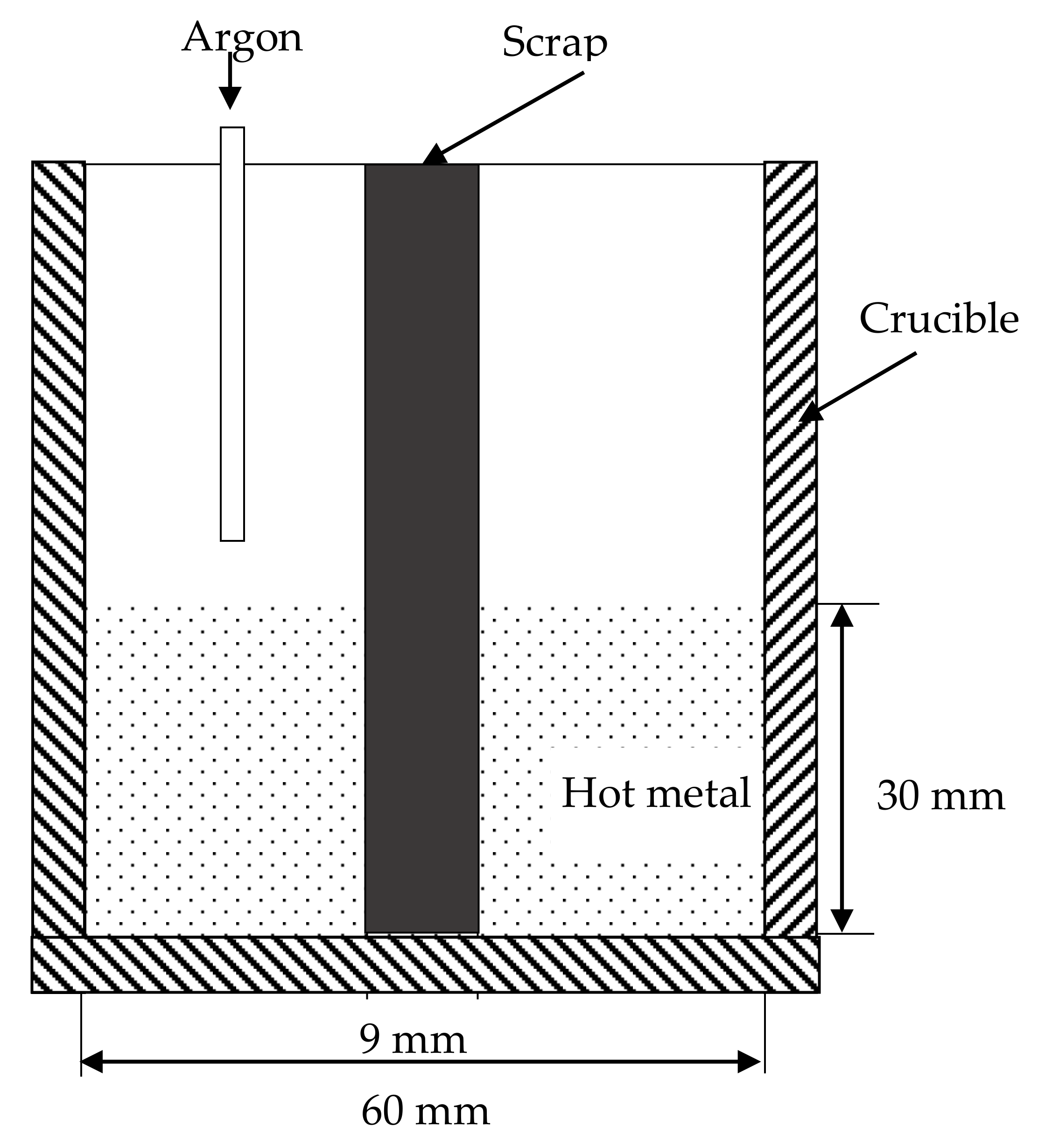
3.1. Experiment

The effects of temperatures and melting times on the melting volume of scrap were investigated in the current study. Experimentally, the scrap melting in the hot metal was performed with the help of a muffle furnace, as shown in Figure 1. Firstly, the crucible filled with solid pig iron was put into the furnace when the muffle furnace reaches the target temperature. The argon which was used as the shield gas, was blown into the crucible through a tube during the whole melting process. Secondly, the scrap bar was inserted into the hot metal bath to melt for a certain time according the experimental schemes, then the bar was drawn out from the hot metal and cooled in a vessel filled with water. The main composition of the hot metal and the scrap bar used in the experiments are shown in

Table 1. The composition of the hot metal and the scrap bar used in the experimental parameters.

Material	C	Si	Mn	P	S
Hot metal	4.01	4.3	0.3	0.014	0.018
Scrap bar	0.1	0.2	0.02	0.016	0.02

. In the experiments, different temperature and melting times were investigated and more details are listed in

Table 2. The operation parameters used in the experiments.

Property	Quantity	Units
Temperature the hot metal	1350, 1400	°C
Temperature the scrap	25	°C
Melting time	30, 60, 90, 120, 150, 180, 210	s
Diameter of the scrap	9	mm

.

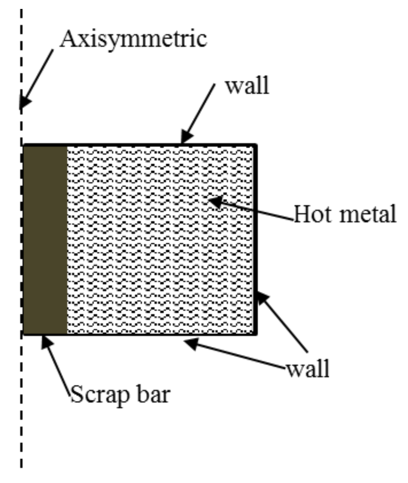
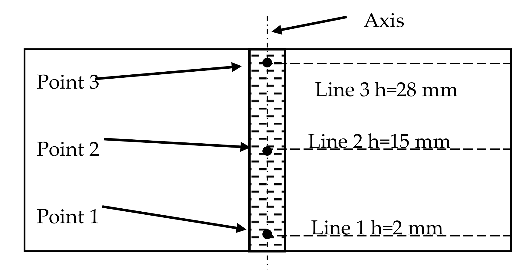
3.2. Mathematical Modeling

Accordingly, a mathematical model was built based on the experimental condition to investigate more parameters which may affect the melting of the scrap bar. A 2-D axisymmetric model was employed to describe the melting process of the scrap bar in the hot metal. To simplify the calculation, a wall function was applied above the molten hot metal instead of the shield gas phase of the experiment in the mathematical model, as shown in Figure 2. The temperature of the top wall was set to be 10 °C lower than that of the bath temperature according experimental measurements. The temperature of the side wall and the bottom wall of the crucible were the same with the temperature of the furnace ambient. The mathematical model performed the phenomena from the time that the bar was immerged in the bath to the time that the bar melting was finished, so the initial bar temperature was set to be the same with the room temperature (25 °C). The initial carbon content of the bar and the hot metal was 0.1 and 4.0 wt.%, respectively. More physical properties of the steel used in the mathematical model are shown in

Table 3. Physical properties used for the simulations.

Property	Quantity	Units
Melting point of pure iron	1805.1	K
Viscosity	0.0062	Pa·s
Equilibrium partition coefficient	0.36	-
Specific heat	500	J/(kg·K)
Thermal conductivity	34	W/(m·K)
Latent heat	2.71 × 105	J/kg
Thermal expansion coefficient	1.07 × 10−4	K−1
Solutal expansion coefficient	1.4 × 10−2	Wt.%−1
Diffusion coefficient in liquid	2.0 × 10−8	m2/s
Diffusion coefficient in solid	1.0 × 10−9	m2/s

. Three bath temperatures of 1350, 1400, and 1450 °C were considered to study the temperature effects on the melting behaviors. The other investigating parameters for the scrap bar used in the mathematical model are the same with that of the experiments, as shown in

Table 4. Investigation parameters of the mathematical simulations.

Property	Quantity	Units
Initial temperature the hot metal	1350, 1400, 1450	°C
Initial temperature the scrap	25	°C
Initial carbon content of the hot metal	4.0	wt.%
Initial carbon content of the scrap	0.1	wt.%
Initial diameter of the scrap	9	mm

.

In the mathematical calculation, the grid density is relatively higher in the region where the melting may occur. The number of cells in the calculation domain is typically about 1.8 × e⁵–2.0 × e⁵. A transient solver with a time step of 1 × e⁻⁴ s was applied to capture the melting behaviors at different times. The PISO (Pressure–Implicit with Splitting of Operators)algorithm was chosen as the Pressure–Velocity coupling method in the current model. Beside, second order upwind was used to consider the momentum, energy, and carbon calculation. In addition, some monitor lines and points were applied to analyze the variation of the interesting parameters during the transient calculation.

4. Results and Discussion

In the experiments, the melting condition at different melting times were investigated with two bath temperatures. Then the mathematical results were verified with the experimental results and applied to investigate more factors and to study the specific phenomena in the melting process, such as temperature distribution, bath flow and distribution of carbon concentration.

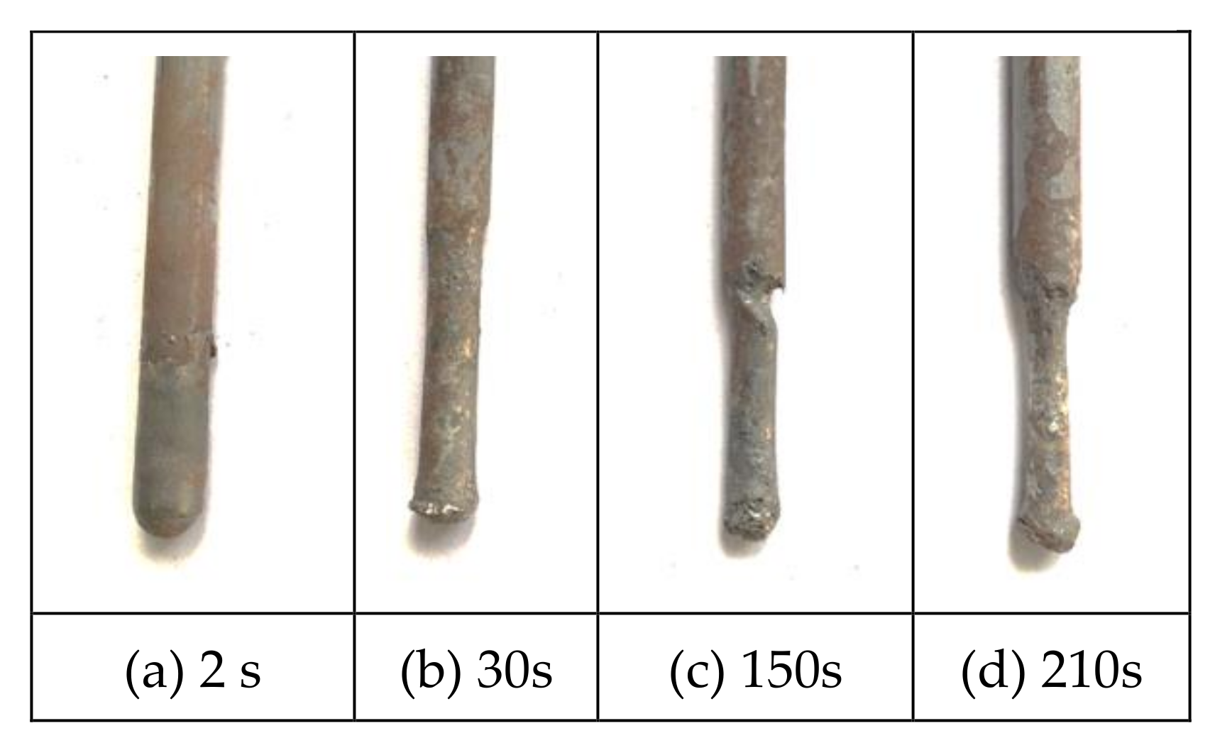
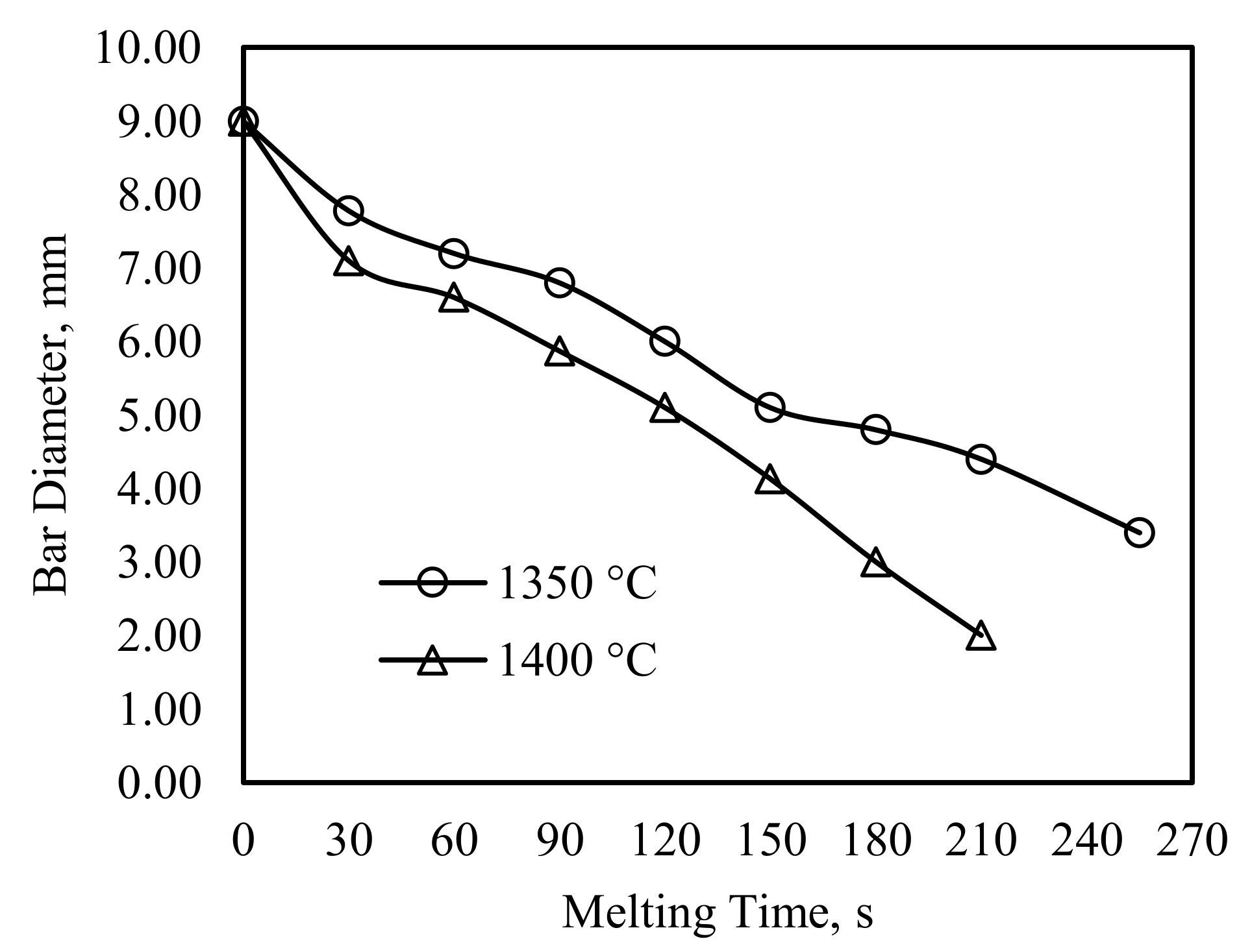
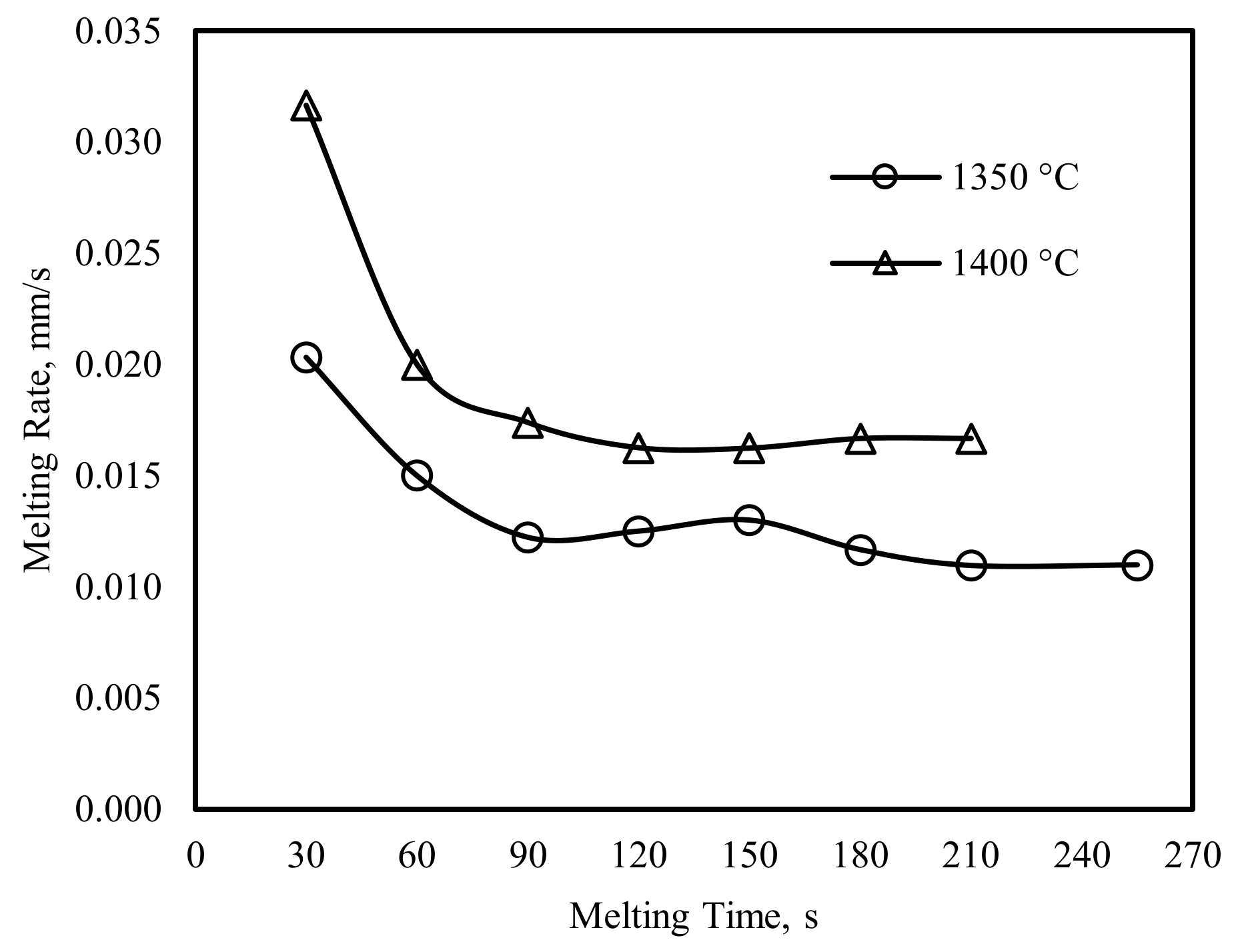
4.1. The Experimental Results and Discussions

The results demonstrate that, firstly, the scrap bar may melt under conditions where the temperature of the hot metal is lower than that of the melting point of the scrap bar, as shown in Figure 3. The diameter of the scrap bar is decreased when the melting time is increased. The diameter changes of the scrap bar are shown in Figure 4, the values shown in the figure is an average diameter of the melting bar at three different vertical levels. Apparently, the diameter of the bar with bath temperature of 1400 °C is smaller than that of the bath temperature of 1350 °C at the same immersion time, which means that increasing melting temperature can increase the melting rate of the bar.

The melting rate of the scrap is not a constant due to the carbon concentration and temperature contribution, as well as the bath flow caused by the nature convection flow in the hot metal bath. Figure 5 shows the melting rate of the scrap bar with different melting times at different temperature of hot metal bath. It shows a rapid melting rate during the melting time region from intitial to 90 s and the melting rate is decreased as the immersion time increased. When the bath temperature is 1400 °C, the melting rate is about twice during the first 30 s over that of the first 90 s. And the melting rate is nearly a constant between 0.010 and 0.015 mm/s after 90 s for both bath temperatures.

Also, the results showed suggest that the melting volume of the scrap bar in the vertical direction is not a constant, similar result can be found in Wei’s research [7], but the details was not discussed in the literature. This demonstrates that the melting rate of the bar is not a constant in the vertical direction during the melting process.

Above results and discussions indicate that the factor that dominates the melting rate in the whole melting process is changed. It can be attributed to the carbon concentration, temperature disctribution, or the flow of the bath. Unfortunately, it is difficult to investigate the factor change during the melting process by applying the experiment. As a result, the mathematical model, with which the carbon concentration, bath flow and so on can be reflected more easily, shall be performed to study more details in the melting of the scrap bar. The details about this phenomena will be discussed in the section below with the help of mathematical simulations.

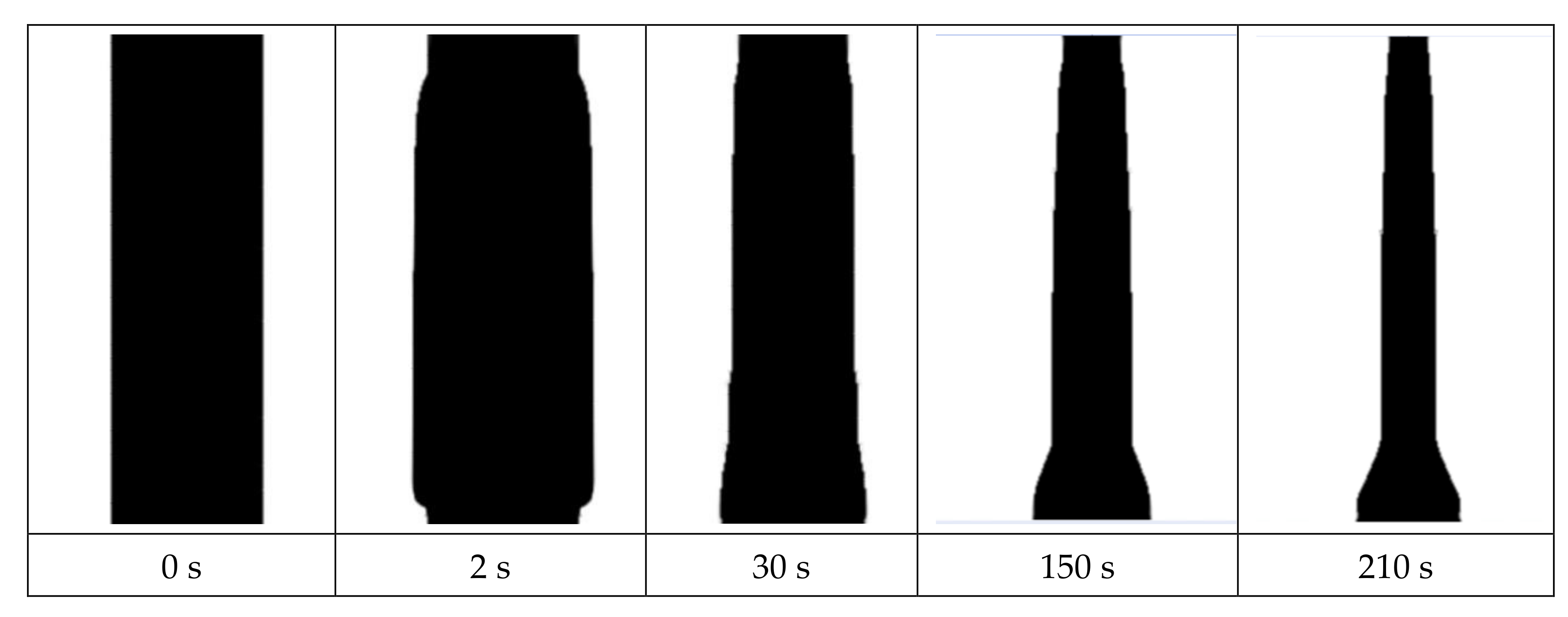
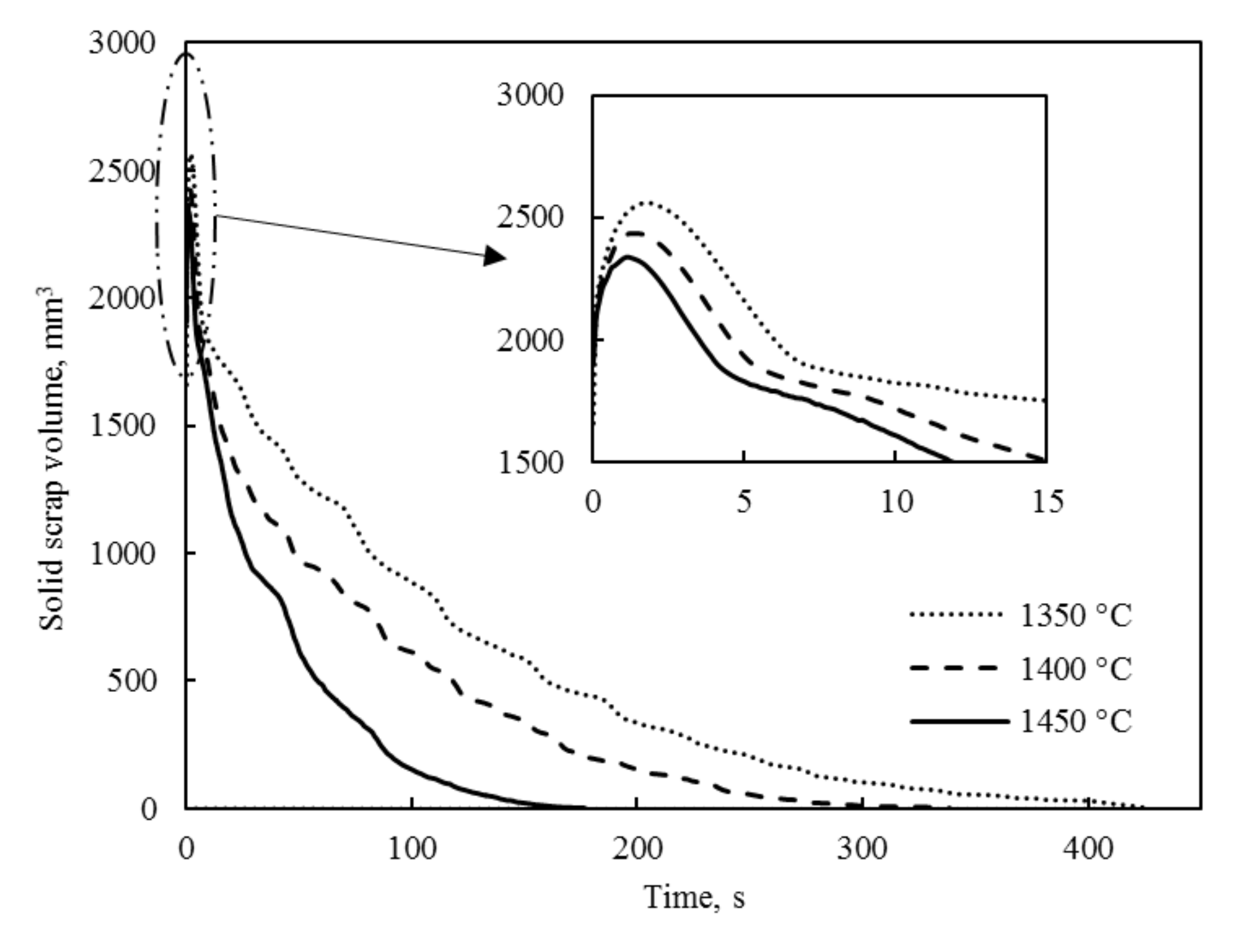
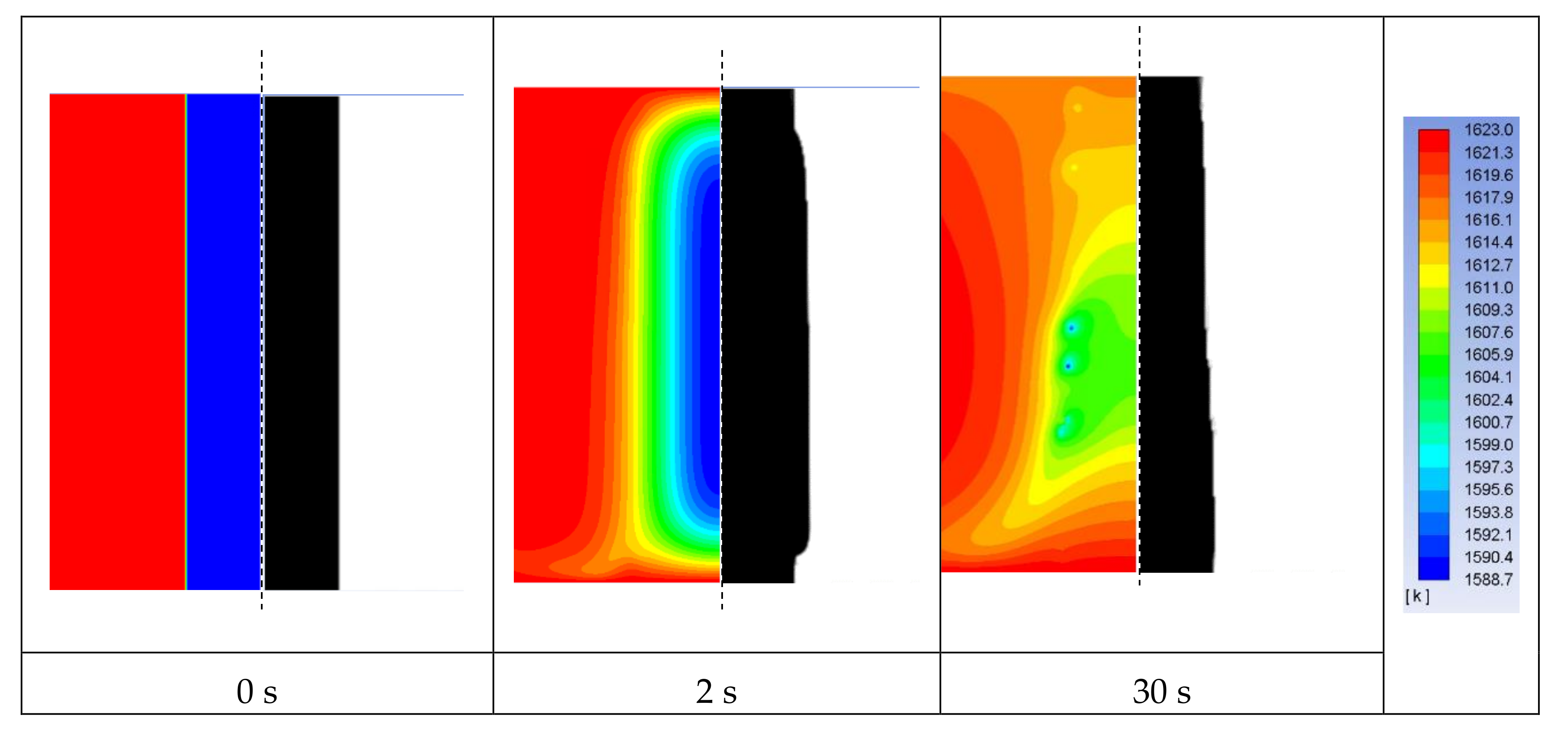
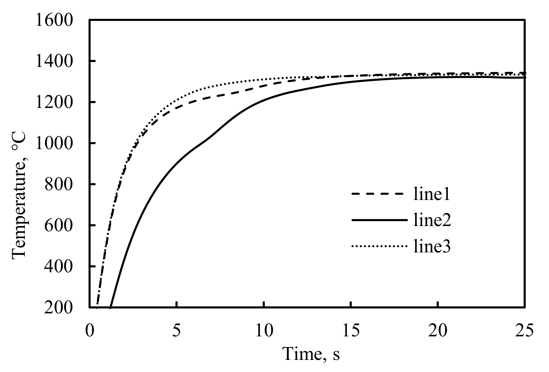
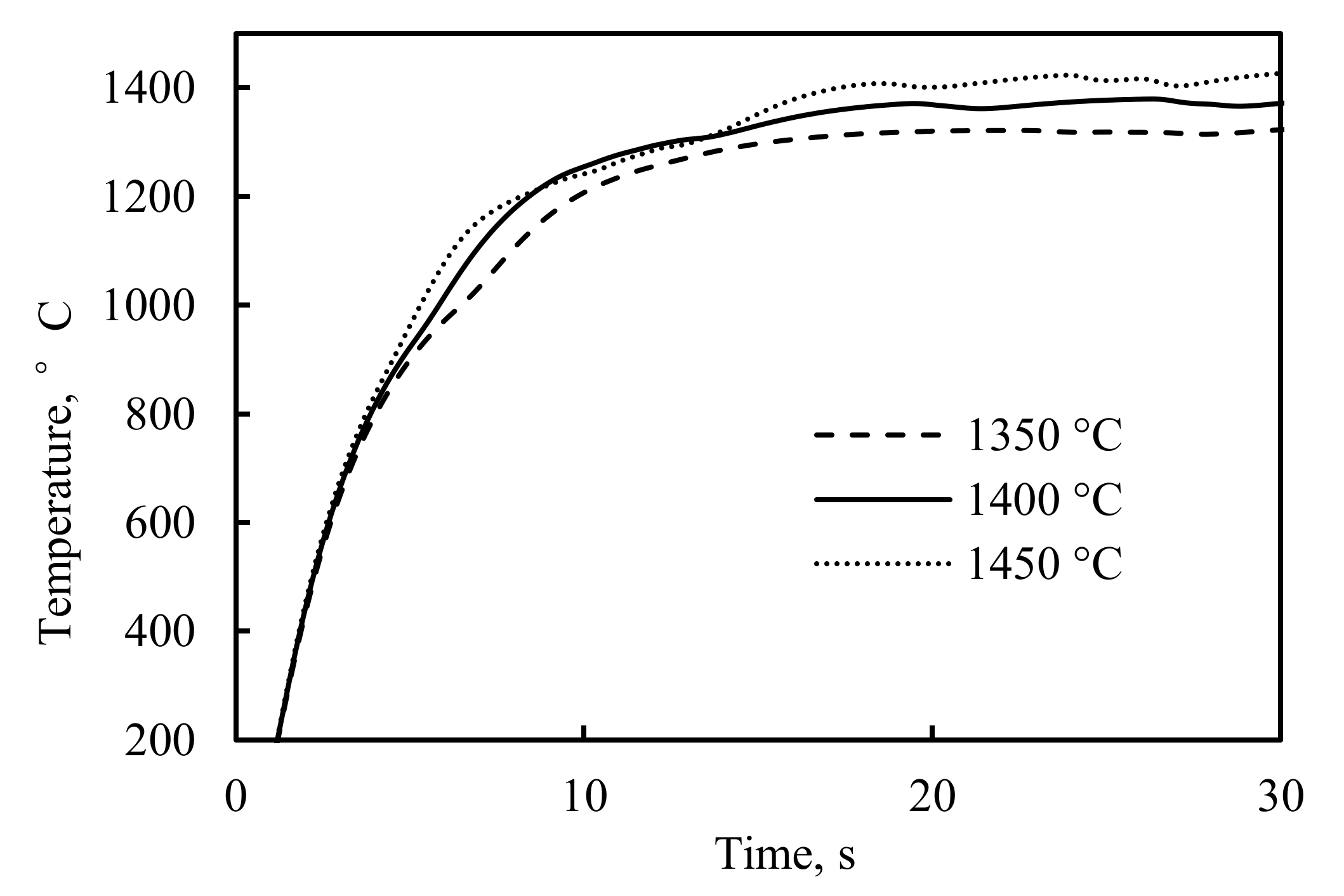
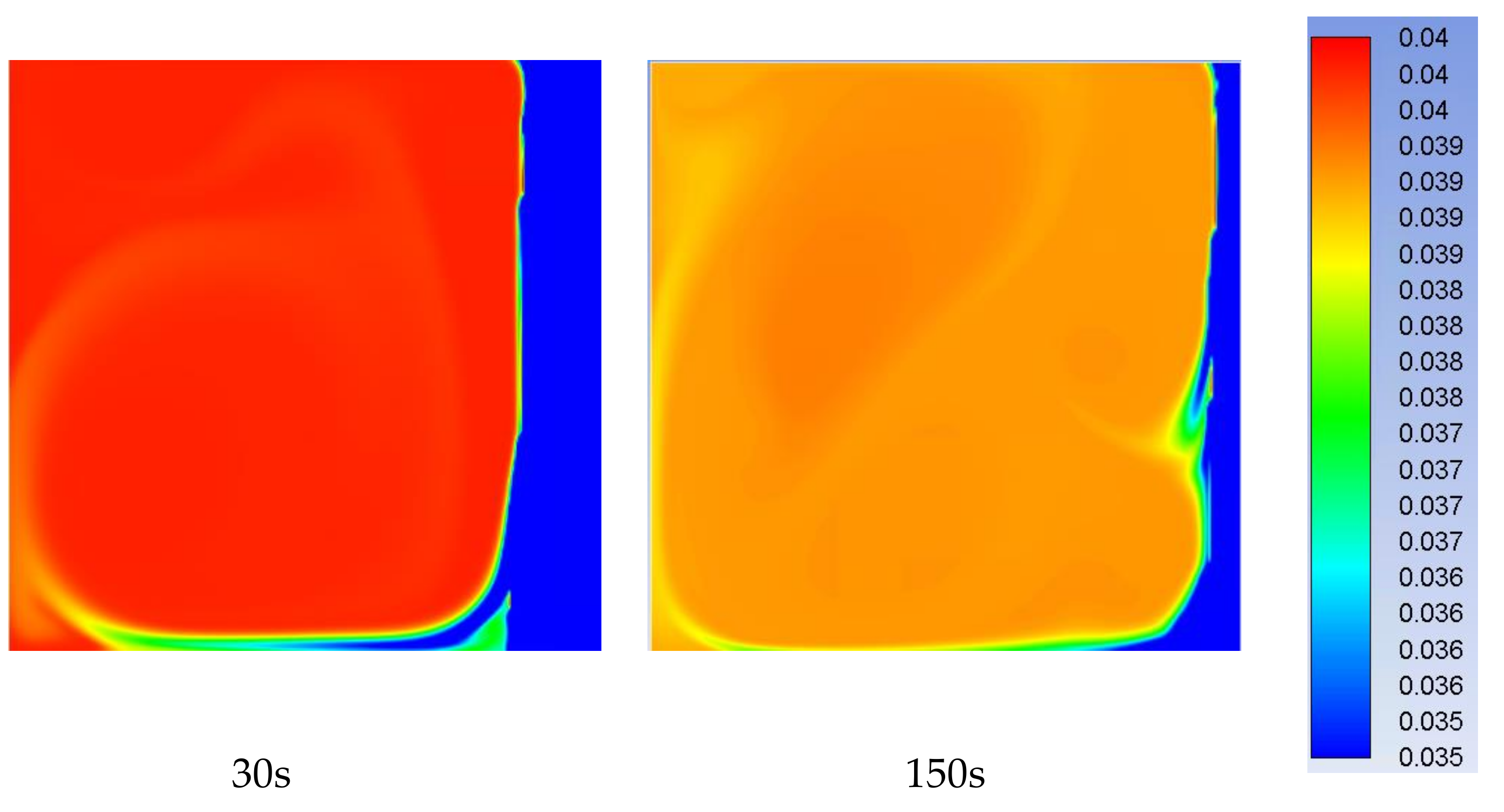
4.2. The Mathematical Results and Discussions

To fully understand the variations of the considered parameters in the bath, three monitor points and monitor lines were applied in the calculation domain to analyze the parameter changes of the bar and the bath temperatures, the bar diameters, the carbon distributions, and the bath flow, the monitor positions are shown in Figure 6.

Figure 7 shows the bar profiles at different melting times when the bath temperature is 1350 °C. Initially, a solid shell was formed at the surface of the scrap bar when the bar was immerged in the bath. Then, the solid shell begin to melt as the temperature was increased up to its melting point with time going. Remarkably, similar phenomena can be observed that the melting rate along the vertical direction is not a constant, compared to the results of the experiments. The melting rate near the upper surface is higher than that of the region in the vicinity of the crucible bottom. More details about the change of the bar diameter at different position are shown in Figure 8. It shows that the diameter of the bar in the upper part (line 1) is smaller than that of the middle part (line 2), followed by the down part (line 3).

The average values of the diameter at three monitor lines was calculated and shown in Figure 8. Compared to the experimental results shown in Figure 4, it shows the variation are in a range of 2–12% for the discrete melting times in the experiment. The causes of the differences between the experimental and mathematical results could be the temperature distribution of the crucible, minor movement or position of the bar, the effects of minor elements in the hot metal and the scrap bar, or other manual operations. In addition, the mathematical model would also arise some errors that would cause the deviations of the results.

The volume changes of the bar were also analyzed to further study the behavior of the bar during the melting process, the results are shown in Figure 9. As shown in figure, originally, the volume of the scrap bar is approximately 1660 mm³. Because the initial temperature of the scrap is room temperature, a solid shell is formed when the bar is immerged in the hot metal. As a result, the solid volume is increased and then decreased when the temperature of the solid shell reaches its melting point under the condition of heat transfer. The maximum values of the solid phase are 2562, 2432, and 2338 mm³ when the initial temperature of the hot metal are 1350, 1400, and 1450 °C, increasing about 54%, 46%, and 40%, respectively. This suggests that more solid shell would be formed around the scrap when the bath temperature is relatively low. Consequently, it is recommended that the volume of the scrap added into the hot metal ladle or the torpedo car should be designed carefully to avoid the melting and flow problem since the temperature of the hot metal is normally low compared the condition in a BOF.

The diameter change of the bar has a significant relationship with the temperature distribution of the bath and the bar. As a result, the temperature distribution and variation during the melting process are analyzed to investigate the relationship between temperature and melting profile of the bar. Figure 10 shows the bar diameter changes the temperature distribution at corresponding melting times when the melting temperature is 1350 °C. It demonstrates that the solid shell formed on the surface of the bar is caused by the low temperature of the bar when the bar is immerged into the bath at the first several seconds. And the temperature at the upper and down part of the bar is normally higher than that of the middle part.

More specific information about the temperature distribution and variation of the bar are summarized in Figure 11 and Figure 12. Figure 11 shows the temperature changes at three monitor points during the melting process when the melting temperature is 1350 °C. It can be seen that the bar temperature increases rapidly from room temperature to a temperature above 1300 °C during the initial 20 s of the melting process. And the temperature at monitor point 1 and 3 are higher than that of the point 2. This demonstrates that the temperature at the middle part of the bar is relatively lower than that of others. The temperature at three monitor points become closer at about 20 s and change slightly after 20 s, which means that the main factor that affects the bar melting is not the temperature but others after this time.

Figure 12 illustrates the temperature increase at the middle of the bar (monitor point 2) when the melting temperature are 1300, 1350, and 1400 °C during the initial melting process. It shows that the temperatures in the bar increase to the temperature close to the bath temperature in about 20 s.

Figure 10 also shows that the temperature at 30 s is not a regular distribution. This is largely influenced by the temperature difference in the bath and the bath flow, which is shown in Figure 13. It can be seen that a flow circulation the crucible bath was formed during the melting process. Typically, the molten hot metal flow along the melting interface from the upper side to the bottom side of the bar. This increases the heat transfer rate of the bath, in turn, affects the temperature distribution of the bar and the interface. The figure also shows that the differences of the flow pattern at the melting times between 30 and 150 s shows that the flow in the bath is changing during the melting process because of the temperature distributions and the changing of the solid bar profiles.

The flow formed in the bath not only affects the heat transfer in the bath, but also the carbon distribution at the interface of the melting. As a result, the melting rate along the interface is changing during the melting process, as shown in Figure 14. Because the molten hot metal flows from the surface of the bath to the bottom along the interface side, the melting phase of the bar is driven away from the interface by the flow. Consequently, the carbon concentration at melting interface of the upper part of the bar is close with that of the bath metal, which is favorable for the further melting of the bar. However, because the melting phase driven by the flow flows along the melting interface, the flow of which the carbon concentration is lower than that of the bath metal. As a result, the melting rate in the down part is relatively lower than that of the upper part of the bar. This illustrates the phenomena found in the experimental and simulation results that the melting rate of the bar in the upper par is higher than that of the down part. The results also suggest that the factor that dominates the process is the carbon concentration distributed in the vicinity of the melting interface, if the temperate during the process is relatively stable.

5. Conclusions

In this study, the scrap melting in the hot metal with high carbon content under different melting temperatures were investigated by carrying on experiments and numerical models. The main conclusions may be summarized as follows.

The experiments demonstrate that the steel can be melted under its melting point when the bar is immerged in the hot metal which contains a high concentration of carbon. The melting rate of the bar at the initial time is relatively higher while it becomes nearly a constant after about 90 s for the current conditions during melting.

Both the experimental and mathematical results show a similar phenomenon that the bar profile is no long a cylinder when the melting process is performed. Based on the simulation results, a circulation is formed during the melting process. As a result, the carbon concentration distribution is affected in the bath and at the interface region. This, in turn, influences the melting rate along the bar in the vertical direction.

The current study shows the temperature distributions of the bath and the effects of temperature on the melting behaviors during the melting process. Also, the effects of carbon content in the bar and bath metal were considered. However, more research on this topic needs to be completed before the association between minor elements and melting behavior is more clearly understood.

References

1. Szekely, J.; Chuang, Y.K.; Hlinka, J.W. The melting and dissolution of low carbon steels in iron carbon melts.pdf. Metall. Trans. 1972, 3, 2825–2833. [Google Scholar] [CrossRef]
2. Kim, Y.U.; Pehlke, R.D. Transient heat transfer during initial stages of steel scrap melting. Metall. Trans. B 1975, 6B, 585–591. [Google Scholar] [CrossRef]
3. Kawakami, M.; Takatani, K.; Brabie, L.C. Heat and Mass Transfer Analysis of Scrap Melting in Steel Bath.pdf. Tetsu Hagane 1999, 85, 20–27. [Google Scholar]
4. Yamamoto, T.; Ujisawa, Y.; Ishida, H.; Takatan, K. operation and design of scrap melting process of the packed bed type. ISIJ Int. 1999, 39, 705–714. [Google Scholar] [CrossRef]
5. Li, J.; Brooks, G.; Provatas, N. Kinetics of Scrap Melting in Liquid Steel. Metall. Mater. Trans. B 2005, 36, 293–302. [Google Scholar] [CrossRef]
6. Li, J.; Provatas, N. Kinetics of Scrap Melting in Liquid Steel: Multipiece Scrap Melting. Metall. Mater. Trans. B 2008, 39, 268–279. [Google Scholar] [CrossRef]
7. Wei, G.; Zhu, R.; Tang, T.; Dong, K. Study on the melting characteristics of steel scrap in molten steel. Ironmak. Steelmak. 2019, 46, 609–617. [Google Scholar] [CrossRef]
8. Sethia, G.; Shuklaa, A.K.; Dasb, P.C.; Chandrab, P.; Deo, B. Theoretical aspects of scrap dissolution in oxygen steelmaking converters.pdf. AISTech Proc. 2004, 2, 915–926. [Google Scholar]
9. Shukla, A.K.; Deo, B.; Millman, S.; Snoeijer, B.; Overbosch, A.; Kapilashrami, A. An Insight into the Mechanism and Kinetics of Reactions In BOF Steelmaking: Theory vs. Practice. Steel Res. Int. 2010, 81, 940–948. [Google Scholar] [CrossRef]
10. Arzpeyma, N.; Widlund, O.; Ersson, M.; Jönsson, P. Mathematical Modeling of Scrap Melting in an EAF Using Electromagnetic Stirring. ISIJ Int. 2013, 53, 48–55. [Google Scholar] [CrossRef] [Green Version]
11. Kruskopf, A. A Model for Scrap Melting in Steel Converter. Metall. Mater. Trans. B 2015, 46, 1195–1206. [Google Scholar] [CrossRef]
12. Shukla, A.K.; Deo, B.; Robertson, D.G.C. Scrap Dissolution in Molten Iron Containing Carbon for the Case of Coupled Heat and Mass Transfer Control. Metall. Mater. Trans. B 2013, 44, 1407–1427. [Google Scholar] [CrossRef]
13. Guo, D.; Swickard, D.; Slavanja, M.; Bradley, J. numerical simulation of heavy scrap melting in BOF steelmaking. In Proceedings of the Iron & Steel Technology Conference and Exposition, Atlanta, GA, USA, 7–10 May 2012; pp. 125–132. [Google Scholar]
14. Ramirez-Argaez, M.A.; Conejo, A.N.; López-Cornejo, M.S. Mathematical Modeling of the Melting Rate of Metallic Particles in the EAF under Multiphase Flow. ISIJ Int. 2015, 55, 117–125. [Google Scholar] [CrossRef] [Green Version]
15. Pineda-Martínez, E.; Hernández-Bocanegra, C.A.; Conejo, A.N.; Ramirez-Argaez, M.A. Mathematical Modeling of the Melting of Sponge Iron in a Bath of Non-reactive Molten Slag. ISIJ Int. 2015, 55, 1906–1915. [Google Scholar] [CrossRef] [Green Version]
16. Berjeza, N.A.; Misuchenko, N.I. Computational Modelling of Heat/Mass Transfer Near the Liquid-Solid Interface During Rapid Solidification of Binary Metal Alloys Under Laser Treatment. Can. Metall. Q. 2013, 37, 313–321. [Google Scholar] [CrossRef]
17. Ludwig, A.; Wu, M. Modeling of globular equiaxed solidification with a two-phase approach. Metall. Mater. Trans. A 2002, 33, 3673–3683. [Google Scholar] [CrossRef]
18. Wu, M.H.; Ludwig, A.; Luo, J.L. Numerical Study of the Thermal-Solutal Convection and Grain Sedimentation during Globular Equiaxed Solidification. Mater. Sci. Forum 2005, 475–479, 2725–2730. [Google Scholar]
19. Wu, M.; Ludwig, A. Using a Three-Phase Deterministic Model for the Columnar-to-Equiaxed Transition. Metall. Mater. Trans. A 2007, 38, 1465–1475. [Google Scholar] [CrossRef]
20. Li, J.; Wu, M.; Ludwig, A.; Kharicha, A. Simulation of macrosegregation in a 2.45-ton steel ingot using a three-phase mixed columnar-equiaxed model. Int. J. Heat Mass Transf. 2014, 72, 668–679. [Google Scholar] [CrossRef] [Green Version]
21. Wu, M.; Li, J.; Ludwig, A.; Kharicha, A. Modeling diffusion-governed solidification of ternary alloys—Part 1: Coupling solidification kinetics with thermodynamics. Comput. Mater. Sci. 2013, 79, 830–840. [Google Scholar] [CrossRef] [Green Version]
22. Li, J.; Wu, M.; Hao, J.; Ludwig, A. Simulation of channel segregation using a two-phase columnar solidification model—Part I: Model description and verification. Comput. Mater. Sci. 2012, 55, 407–418. [Google Scholar] [CrossRef]
23. Moelans, N.; Blanpain, B.; Wollants, P. An introduction to phase-field modeling of microstructure evolution. Calphad 2008, 32, 268–294. [Google Scholar] [CrossRef]
24. Fluent User’s Manual; ANSYS: Canonsburg, PA, USA, 2018; pp. 646–648.
25. Voller, V.R.; Brent, A.D.; Reid, K.J. A Computational Modeling Framework for the Analysis of Metallurgical Solidification Process and Phenomena. Technical report. In Proceedings of the Conference for Solidification Processing Ranmoor House, Sheffield, UK, 21–24 September 1987. [Google Scholar]
26. Voller, V.R.; Prakash, C. A Fixed-Grid Numerical Modeling Methodology for Convection-Diffusion Mushy Region Phase-Change Problems. Int. J. Heat Mass Transf. 1987, 30, 1709–1720. [Google Scholar] [CrossRef]
Figure 1. Schematic of the experiments.
Metals 10 00678 g001
Figure 2. The calculation domain of the mathematical model.
Metals 10 00678 g002
Figure 3. Appearance of the steel bar after immersion in the hot metal: (a) 2 s, (b) 30 s, (c) 150 s, (d): 210 s.
Metals 10 00678 g003
Figure 4. Diameter change of the scrap bar at different bath temperatures.
Metals 10 00678 g004
Figure 5. Melting rate of the scrap bar with different melting times.
Metals 10 00678 g005
Figure 6. Monitor positions during the melting process.
Metals 10 00678 g006
Figure 7. The bar profiles at different melting times.
Metals 10 00678 g007
Figure 8. The changes of bar diameter at different monitor positions.
Metals 10 00678 g008
Figure 9. The volume variation of the solid scrap during the melting process.
Metals 10 00678 g009
Figure 10. The diameter change and temperature distribution of the bar during the melting process.
Metals 10 00678 g010
Figure 11. The temperature increase of the bar at different monitor points for the melting temperature of 1350 °C.
Metals 10 00678 g011
Figure 12. The temperature increase of the bar at monitor point 2 for different melting temperature.
Metals 10 00678 g012
Figure 13. The flow fields (a) and contours (b) of the bath at different melting time for 1350 °C.
Metals 10 00678 g013
Figure 14. The carbon concentration distribution in the bath at different melting times at 1350 °C.
Metals 10 00678 g014