Article

Experimental and Numerical Analysis of Gas/Powder Flow for Different LMD Nozzles

1
Laboratoire PIMM, UMR 8006 ENSAM-CNRS-CNAM, HESAM Université, 151 boulevard de l’hôpital, 75013 Paris, France
2
Centre des Matériaux, Mines Paristech, CNRS UMR 7633, 63–65 rue Henry-Auguste Desbrueres, 91103 Evry, France
3
Safran Additive Manufacturing, Technology platform of Safran Tech, Rue des Jeunes Bois, Châteaufort, 78114 Magny-Les-Hameaux, France
*
Author to whom correspondence should be addressed.
Metals 2020, 10(5), 667; https://doi.org/10.3390/met10050667
Submission received: 20 April 2020 / Revised: 16 May 2020 / Accepted: 18 May 2020 / Published: 20 May 2020
(This article belongs to the Special Issue Additive Manufacturing of Metals with Lasers)

Abstract

:
The Laser Metal Deposition (LMD) process is an additive manufacturing method, which generates 3D structures through the interaction of a laser beam and a gas/powder stream. The stream diameter, surface density and focal plan position affect the size, efficiency and regularity of the deposit tracks. Therefore, a precise knowledge of the gas/powder streams characteristics is essential to control the process and improve its reliability and reproducibly for industrial applications. This paper proposes multiple experimental techniques, such as gas pressure measurement, optical and weighting methods, to analyze the gas and particle velocity, the powder stream diameter, its focal plan position and density. This was carried out for three nozzle designs and multiple gas and powder flow rates conditions. The results reveal that (1) the particle stream follows a Gaussian distribution while the gas velocity field is closer to a top hat one; (2) axial, carrier and shaping gas flow significantly impact the powder stream’s focal plan position; (3) only shaping gas, powder flow rates and nozzle design impact the powder stream diameter. 2D axisymmetric models of the gas and powder streams with RANS turbulent model are then performed on each of the three nozzles and highlight good agreements with experimental results but an over-estimation of the gas velocity by pressure measurements.

1. Introduction

The recent notion of Rate Per Flight Hour (RPFH) business in aeronautics sectors leads to a wide development of repairing technics for aircrafts maintenance to offer a stronger, faster and cheaper process. Welding technics are frequently used to repair damaged metallic parts. However, they generate a deep Heat Affected Zone (HAZ) and may cause geometric distortions or affect the metallurgy and mechanic strength of the part [1]. The Laser Metal Deposition (LMD), is an emergent DED (Direct Energy Deposition) manufacturing process for which a laser melts a substrate where metallic powder particles are injected, to build 3D structures layer by layers (Figure 1). Recently, this process has received significant attention due to its advantages over the conventional repairing approach: low heat impact [2], material flexibility [3] and a CNC (Computer Numerical Control) or robot integration to automate the process and enhance its reliability. LMD is able to rebuild previously considered non-repairable damaged parts and has been successfully used for gas turbine blades [4] or airfoil’s leading edges of GE’s technic [5] repair demonstrators. However, a sufficient repeatability and reproducibly of the process can still be improved and studies cannot be easily transferred from one machine or nozzle to another. This is due to the considerable number of parameters that govern the powder stream and affect the efficiency, geometry and quality of the deposit [6]. Consequently, intensive studies need to be conducted to understand and control the powder stream generated by the process for multiple process parameters.
The experimental analysis of the powder stream is rather well documented in LMD literature and is usually based on optical methods. The latter combine a narrow laser illumination (“laser sheet”) and a CDD camera to record the intensity of the scattered light. A vertical pencil-like laser light allows the recording of the entire stream coming out of the nozzle and gives the powder jet structure and its particle velocity [6]. Using this technique, Zhu et al. [7] showed the influence of the thickness and external diameter of the nozzle’s powder channel on the jet structure. The work by Takemura et al. [8] showed that the jet diameter (φjet) is limited by a low carrier gas flow rate and adapted the flow rate to ensure an optimal deposition efficiency. With a cylindrical lighting, Wu et al. [9] evidenced an unstable jet and a low process efficiency when the work plan is above the focal plan. Horizontal lighting combined with an additional mirror can also be used for a coaxial 2D view of the stream, in order to obtain the powder flow density (Dms, g·mm2·s−1) by luminance measurements [10]. This powder stream parameter can also be obtained by weighting methods. Thus, by weighting the fraction of the jet that is able to go through a pinhole for different X positions, Gharbi [11] showed that a circular Gaussian-like distribution can describe the powder flow density at the Powder Focal Plan (PFP). Eisenbath et al. [12] used the same system but for multiple X–Y–Z positions of the pinhole below the nozzle to offer a 3D description of the jet. In their work, the powder flow density was found to follow an annular distribution above and below the focal plan, which differs from the nozzle’s size. Liu et al. [13] placed the processing head statically above cylindrical containers with specific concentric holes of different diameters [14] and showed that the powder flow keeps pitot ian distribution within a +/− 2 mm distance to the focal plan. All these experimental studies allow a more or less accurate description of the powder jet structure and density, without clearly establishing a dependency on process parameters or on the nozzle design.
Since the variation in manufacturing configuration is not always easy or possible, numerical studies are needed to understand the impact of specific parameters on the process. A large majority of these numerical works are based on 2D or 3D CFD simulations with turbulent k-ε gas flows for particular set of powder, gas rates and nozzle design. Thus, authors show that shielding gas has a strong impact on the powder stream’s particles density and structure [7] as well as on the quality of the local inert atmosphere of the deposition area [15]. Particle velocity (Vp) and jet convergence were found to be influenced by the particle mean diameter (dp) [16] and the carrier gas flow rate [8]. Experimental Schlieren and high-speed-imaging also highlighted the gas flow velocity (Vg) influence on the laminar or turbulent property of the gas flow as well as on the powder stream’s convergence quality [17]. Furthermore, some numerical studies focused on the nozzle design and injection configuration. The literature shows that the injection angles of disperse nozzles [16] as well as the Z offsets of the coaxial nozzle’s parts [18] directly impact the convergence length and influence the powder supply efficiency. Arrizubieta et al. [19] underlined the formation of an asymmetric powder jet for a coaxial nozzle tilt higher than 30° relative to the vertical axis, which has a significant impact on the direction dependence of the process. The typical patterns of powder density and particle temperature distributions were found to be dependent on the coaxial nozzle type by Kovalev et al. [20]. Considering all these works, it can clearly be established that the nozzle design and gas parameters have a strong impact on the powder flow density, speed and trajectory, and hence directly influence the powder stream characteristics and the clad efficiency [21].
Thus, multiple experimental technics exist to describe the powder stream structure and characteristics but the influence of process parameters such as gas flow rate (Dg), standoff distance (WD) and nozzle design have rarely been studied numerically and compared with experimental data. This paper presents a combined experimental and numerical approach including:
(1)
A 3D pressure measurement with a Pitot tube to describe the gas velocity for 3 nozzle design and multiple gas flow rate;
(2)
A 3D coaxial optical observation combined with a lateral view of the powder stream and a weighting method to efficiently describe the powder stream characteristics for the 3 nozzles and multiple gas flow rates;
(3)
2D axisymmetric simulations of the gas flow, and powder stream.
Special attention was paid to the determination of particle’s velocity, trajectory, powder stream diameter, density and focal plan position.

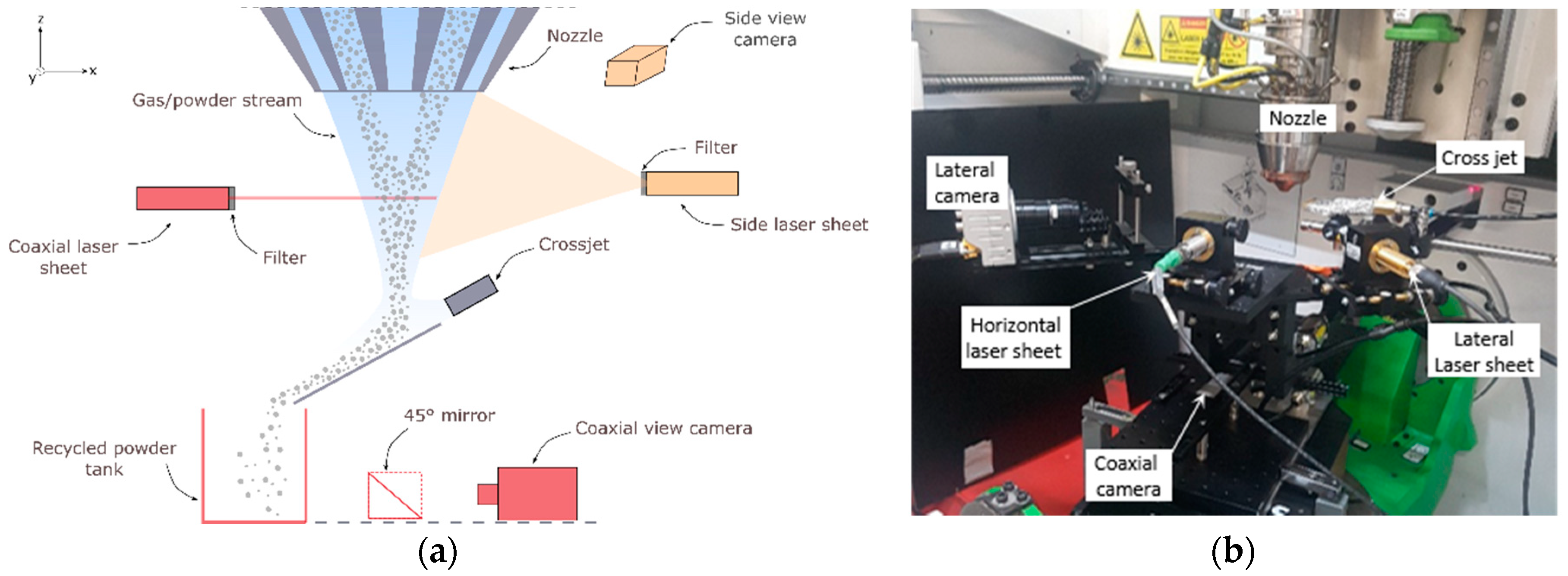
2. Experimental Conditions

The LMD process uses a nozzle with many possible sizes, configurations or geometries depending on the manufacturer or the targeted application. Such nozzles are complex mechanical parts where the laser beam path, the powder stream injection and multiple functional gas flow delivery must be combined. Most nozzles have a coaxial configuration, meaning that the gas-powder stream is injected around the laser beam axis and interact on a vertical distance usually known as the “interaction distance”. This configuration allows a nearly direction-independent deposit and provides large freedom of movement. Depending on the nozzle configuration, two types of powder injection exist: discrete and continuous. For the discrete one, the powder stream is injected by three to four discrete streams, which meet at the powder focal plan (PFP) to generate a dense and focused steam. On the other hand, a continuous powder injection generates a nearly homogeneous conical stream at the nozzle outlet. In the current work, three continuous coaxial nozzles (A, B and C), were tested on two different laser cladding machines. Each nozzle has its own design and its own set of usual parameters.
The first cladding machine is a five-continuous-axes machine equipped with two removable nozzle heads, according to the size of the needed deposit. The first one, “nozzle A”, is the smallest nozzle head of the study. It allows a width deposit of 0.8 to 1.2 mm and is mostly used with a 3.5 mm standoff distance (WD) during the process (Figure 2). The second nozzle, called “nozzle B”, allows a thicker deposit (more than 2 mm), and is usually carried out with a 13 mm standoff distance (Figure 2). These two nozzles share a similar design, with three conic extensions leading to three gas channels:
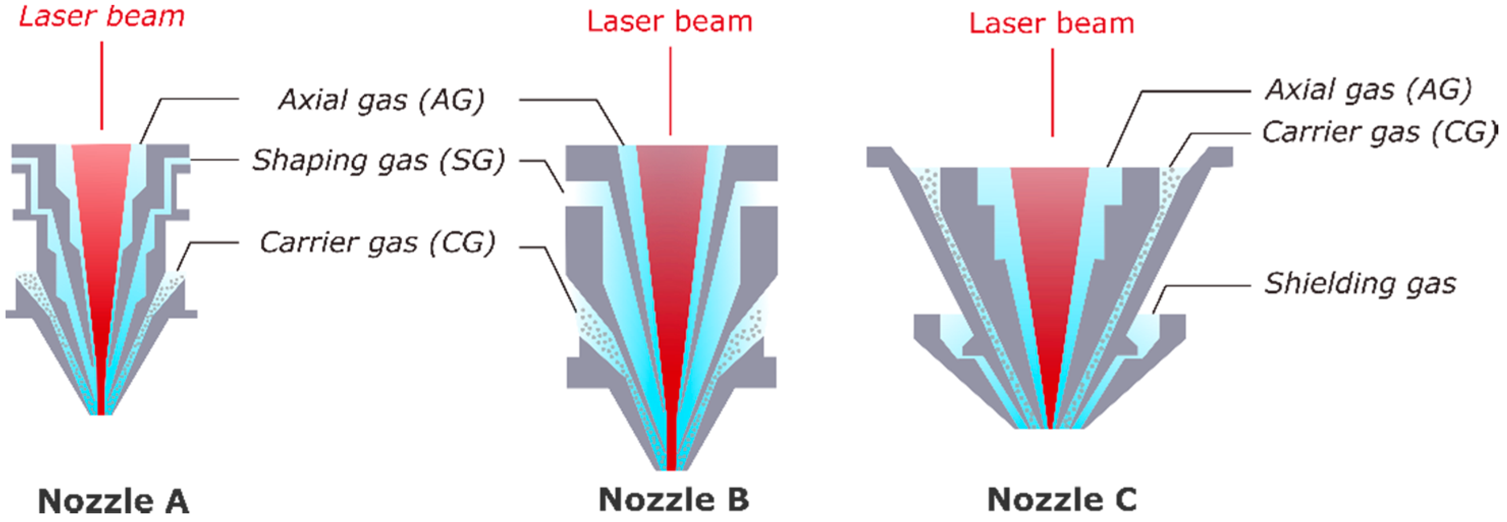
  • An axial gas (AG) channel, to protect the laser beam optics;
  • An internal annular channel, with a shaping gas (SG) which controls the powder stream structure;
  • An external annular channel where a carrier gas (CG) hold the particles inside the nozzle until they reach the shaping flow. The particle flow and its carrier gas are injected in the annular channel by two main entrance points.
The second machine is an instrumented set-up equipped with a custom coaxial deposit head (“nozzle C”) composed of two cones and two distinct gas flows: axial (AG) and carrier gas (CG) (Figure 2). A supplementary third cone, along with a shielding gas, can be added to improve the gas shielding. In this case, the particle stream is injected from four entrance points into the powder channel.
In all cases, each flow injected in the deposit heads is composed of Argon inert gas (Table 1). Standard gas parameters used for each nozzle are exposed in Table 2. Commercial metal powders of an IN718 Ni-based superalloy were used for all the experiments, with a d10 = 51 µm and d90 = 109 µm Gaussian-like particle size distribution and a sphericity close to 0.94.

3. Experimental Results

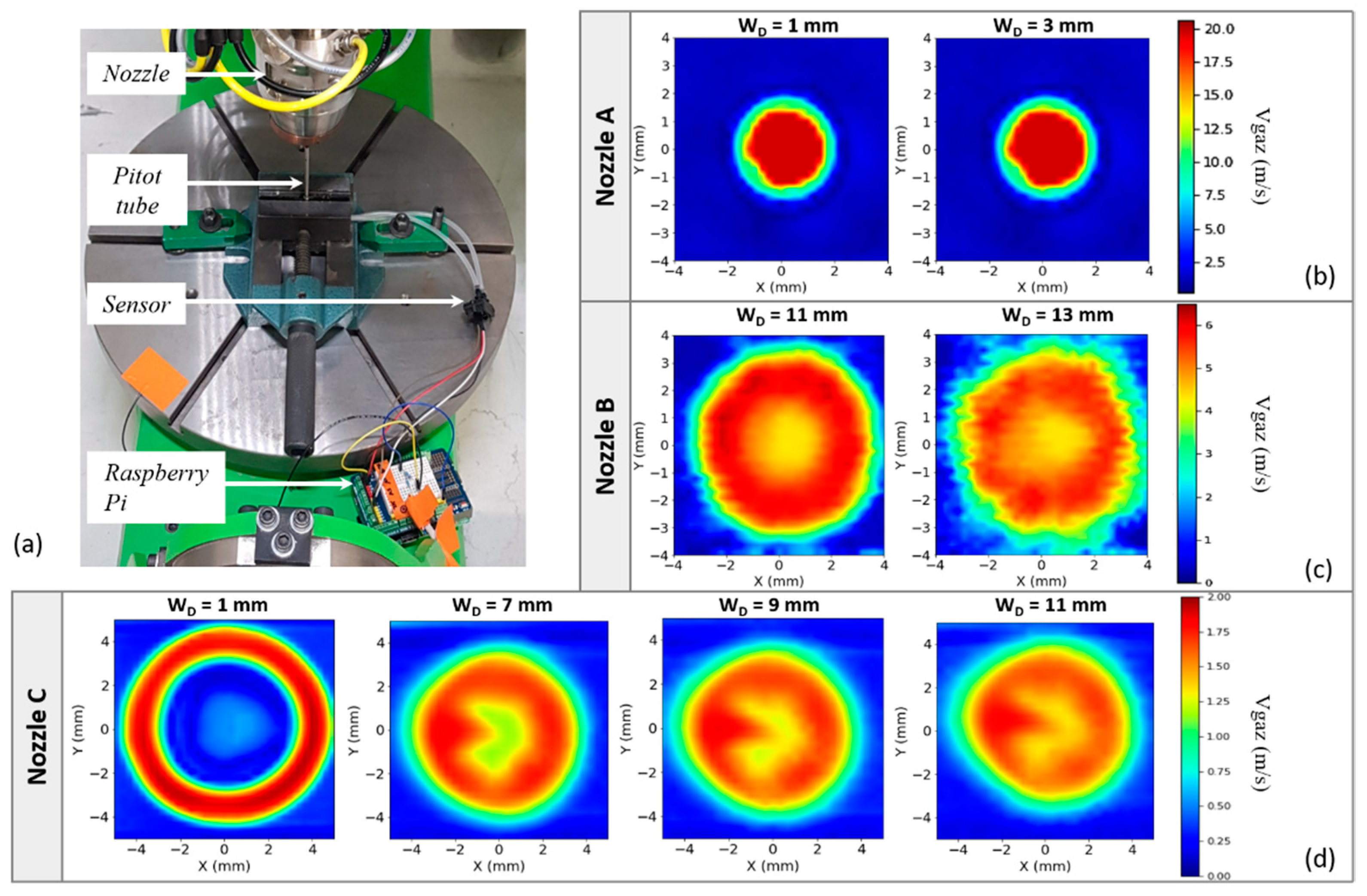
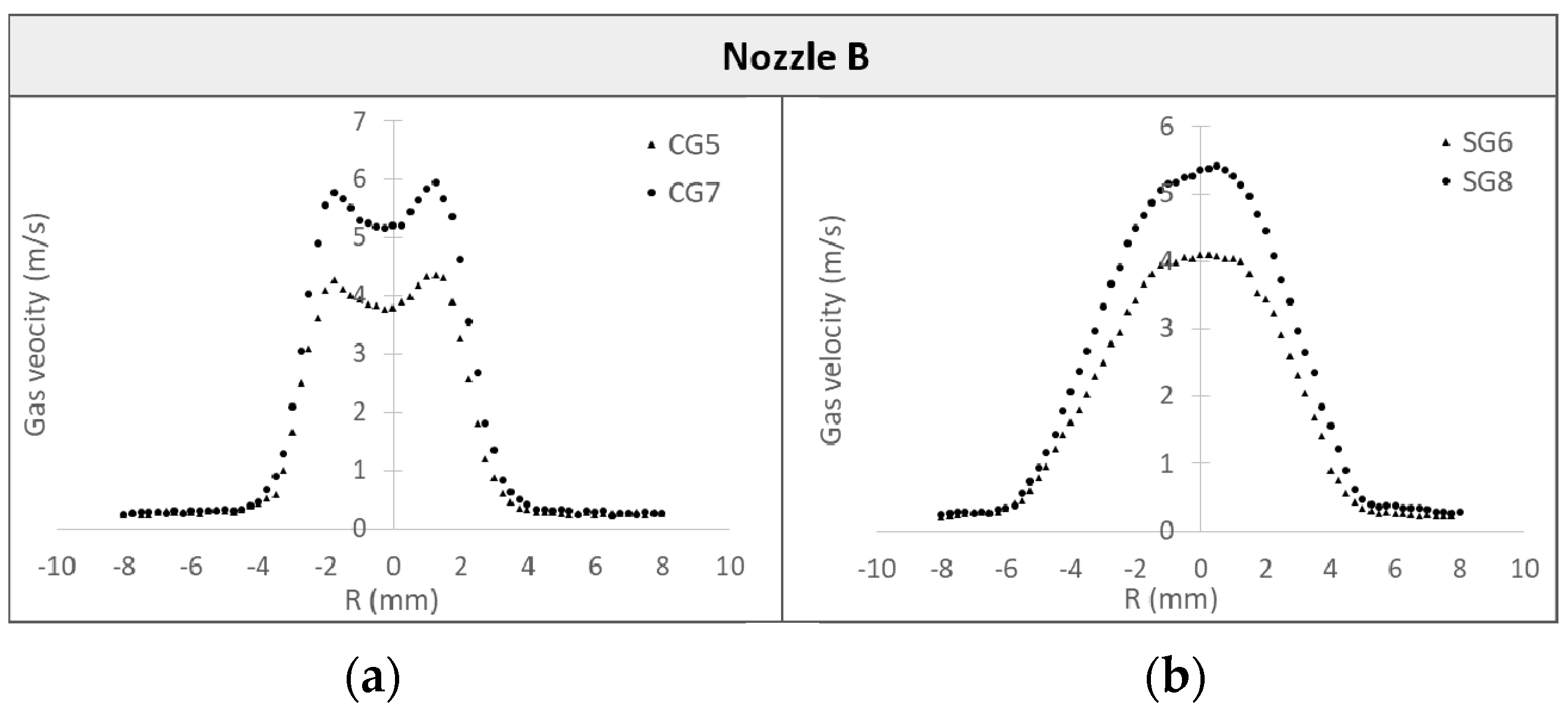
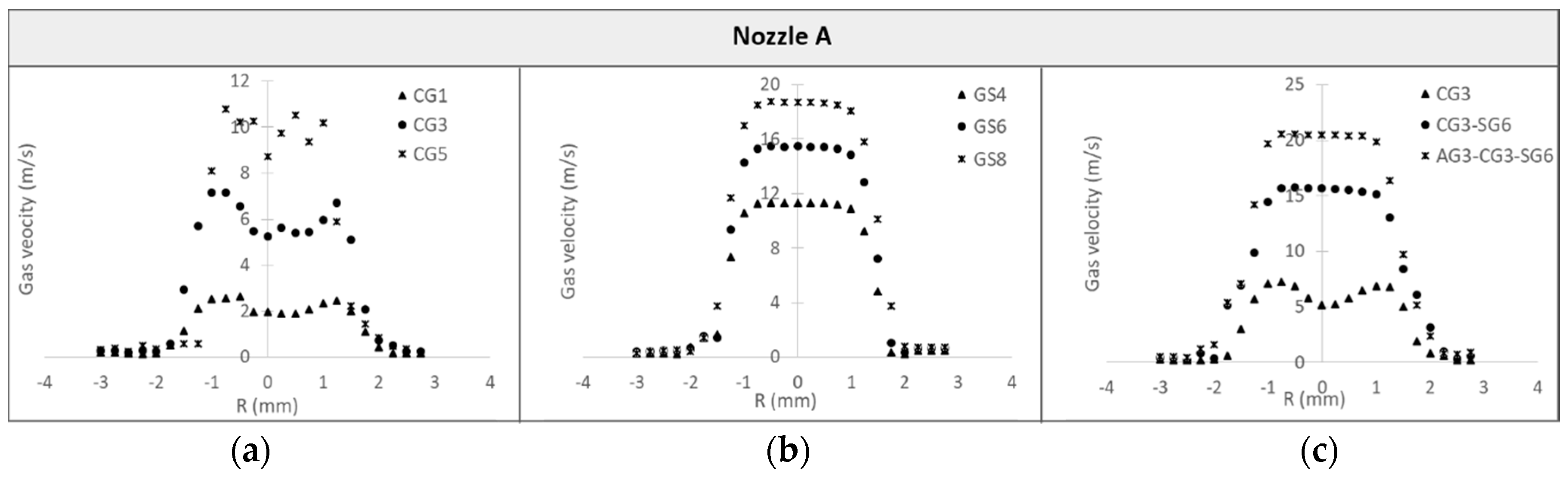
3.1. Gas Velocity Measurement

Since the powder stream is carried and in contact with the gas streams during the whole process, a first step was to investigate the gas stream shape and velocity field. For this study, the gas flow was monitored with an intrusive velocity measurement instrument known as a Pitot tube. It works as a differential pressure anemometer that allows the velocity measurement of a single localized fluid flow [22]. Practically, such a device, widely used to measure aircraft’s speed, is made of a tube with an open end facing the fluid flow (total pressure entrance) and an orifice flush tangential to the tube, which registers the static pressure [23]. The pressure difference between total and static entrance is estimated on the basis that the fluid kinetic energy is fully converted into an increase in pressure. Under most conditions, the drop of pressure between the two orifices can be converted into velocity by Bernoulli’s equation [24]
v = 2   Δ P ρ ,
where ρ is the fluid density and Δ P the pressure difference measured by the pitot tube. Due to its low cost, its compactness and ease of installation, Pitot tubes are used in many industrial fields to measure or control fluid flows. However, their accuracy can be limited for unsteady flows, especially when the viscous effects become too significant (low Reynolds number). Studies by Spelayet al. [22] and Boetcher et al. [25] showed that pitot measurement conducted with a Reynolds number lower than 100 could not be accurately predicted with Bernoulli’s method and needs correlation terms to correct it. In this study, the Reynolds numbers of each gas flow coming out from the three studied nozzles are higher than 1000 for the usual gas process parameters, meaning that the basic Bernoulli’s equation is sufficient to describe the speed flow.
A Pitot tube with an entrance diameter dPitot = 0.5 mm and an internal diameter DPitot = 2 mm was used with sensors of 125 Pa for nozzles B and C and 500 Pa for nozzle A to match the correct orders of magnitude. Before the experiment, the pitot instrument is arranged along the nozzle direction and positioned perpendicularity to the working table (Figure 3a). The centering adjustment between the tube and the nozzles was realized with the coaxial camera of the machine, and the standoff distance between the nozzle and the tube tip was controlled with gauge blocks.
Multiple measuring points following a 2D grid of 3 × 3 to 4 × 4 mm2 were programmed to obtain a velocity mapping Vgas = f(x,y) at the output of the nozzles for various standoff distances. During the experiment, the Pitot tube (or the nozzle head) was displaced of a 0.25 mm distance along the X and Y axis to reach each point of the grid and stopped for 7 s to continuously register data with a Raspberry Pi 3 model B nano-computer (Figure 3a). The velocity maps were interpolated with a bilinear function and tested gas conditions are exposed in Table 3. As an example, in the following, experimental gas conditions will be indicated as: AG6-CG5-SG3 for 6 L/min axial gas, 5 L/min carrier gas and 3 L/min shaping gas.
The recorded maps exhibit the velocity variation of the gas flow along the X and Y axis for several standoff distances, with each nozzle. First, the perfectly circular geometrical shape obtained 1 mm below nozzle C tips (Figure 3d) indicates that the Pitot tube doesn’t interfere with the measurements. Then, the comparison of velocity maps obtained at various standoff distances allows tracing the gas jet caustics.
Results obtained from nozzle C show the gradual variation of the gas flow distribution during its trajectory in the air-based atmosphere at 1, 7, 9 and 11 mm distances below the nozzle outlet (Figure 3d), for AG2-GP4 gas conditions. Because of the convergent shape of its pathway, the jet structure is first annular, then becomes more and more convergent at higher distances from the nozzle outlet. A nearly uniform gas velocity field, close to a “top hat” distribution, is obtained for WD = 9 mm with a maximum velocity of 1.85 m/s. Results show that its maximum velocity and its diameter, which reaches 5 mm, does not evolve for a working distance between 9 and 13 mm.
Experiments on nozzle B were performed around its usual working distance, between 11 and 15 mm below its tips. Results showed a nearly uniform gas velocity field for all investigated working distances for its standard gas conditions (Table 2). The jet reaches a diameter of 7 mm and a maximum velocity of 6.1 m/s (Figure 3c). Figure 4a,b show the gas velocity distribution along the X axis of the jet for a variation in carrier and shaping gas flow rate, respectively. It seems that the carrier gas curve follows an annular Gaussian like distribution, while the shaping gas exhibits a nearly top hat distribution, for the five investigated standoff distances. For both cases, the gas velocity field significantly increase with the carrier and shaping gas flow rate: an increase of 2 L/min approximately leads to a 1.5 m/s rise in the maximum velocity field for WD = 13 mm.
Experiments on nozzle A were also conducted around its usual working distance, between 1 and 5 mm below its tips. Results show a much finer, faster and homogeneous stream than with previous nozzles. For its standard gas conditions (AG3-CG3-SG6), the stream presents a diameter of 3 mm and a maximal velocity of 20.5 m/s (Figure 3b). The velocity field of the jet significantly increases with flow rates: an increase of 2 L/min leads to a 3 and 4 m/s rise in the carrier and shaping gas velocity respectively. As well as nozzle B, the carrier gas velocity distribution along X seems to follow an annular Gaussian distribution (Figure 5a), however, the shaping gas velocity clearly exhibits a top hat distribution for all tested flow rates and standoff distances (Figure 5b,c) shows the influence of the gas channels’ activation, and clearly indicates that the velocity field of the stream follows a top hat distribution as long as the carrier gas is not the only gas flow used for the process.
These results confirm the strong influence of the channels’ geometry on the gas stream diameter and velocity: because nozzle A has the narrowest gas channels of the three nozzles, the output gas stream is faster, finer and more uniform at the nozzle outlet. The gas channels of nozzles B and C, which are larger, limit gas flow velocities at constant flow rate. Finally, the following conclusions can be drawn:
  • The carried gas velocity field alone follows an annular Gaussian distribution for the investigated standoff distance range;
  • When a second gas channel is activated, the velocity field distribution is much closer to a top hat distribution;
  • The stream becomes faster with channels activations and with a rise in their flow rate, without significant changes of the stream diameter;
  • The thinner the gas channels, the faster and the finer the gas stream is.

3.2. Analysis of the Powder Stream

3.2.1. Calibration of the Feeding Rate

The powder mass flow rate (Dm, g·min−1) is an adjustable and essential parameter of the process. With both machines, it is controlled by a powder delivery system based upon the number of revolutions per minute (RPM, %) of a wheel including a feeding kerf. Before each experiment, a calibration curve Dm = f (RPM) was performed by a continuous measurement (3 Hz) of the powder mass exiting the nozzle during a given recording time, with a repeatability of ± 0.01 g in order to adjust the powder mass flow rate as needed. This calibration was performed on all nozzles for four targeted mass flow rates: 4, 6, 8 and 12 ± 0.2 g·min−1.

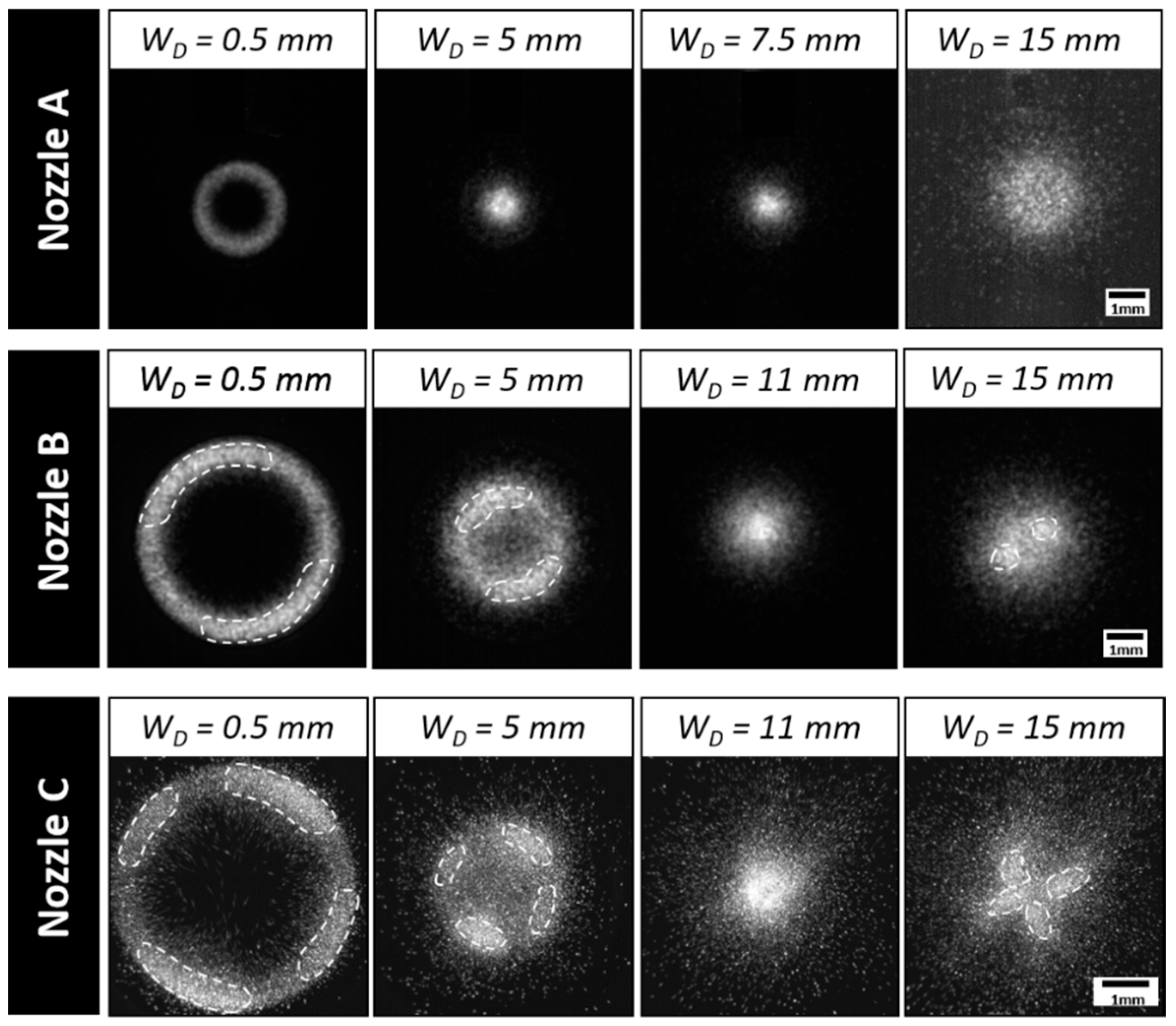
3.2.2. Video Imaging of the Powder Stream

The experimental analysis of the powder stream was performed with a combination of coaxial and lateral views. This requests two sets of cameras and laser lighting (two different wavelengths) and can obtain the particle velocities and the powder stream shape with only one setup. To obtain both views at the same time, a filter is fixed to each camera to only record the particles flowing through the corresponding laser sheet (coaxial or lateral) (Figure 6).
The lateral imaging technique allows a 2D side view (XZ) of the stream. The latter is illuminated by a 650 nm laser sheet and recorded by a high-speed CDD camera (Figure 6). Two evaluation windows were set, one for a total view of the stream (4500 fps, shutter time of 222 µs) (Figure 7c) and another for a more precise and zoomed analysis (12,000 fps, shutter time of 84 µs) (Figure 7a,b).
For the “coaxial” view, the transverse section (XY) of the powder stream is illuminated by a horizontal laser sheet (λ = 450 nm, thickness ~ 200 µm) and captured with a CDD high-speed camera with the help of a 45° mirror positioned below the nozzle (Figure 6). A protective glass window with a gas crossjet is set to deviate the lower part of the stream to protect the mirror and camera setup. The coaxial view was recorded at 200 fps for multiple standoff distances, from 0.5 to 16 mm below the nozzle tip, with a ΔZ increment of 0.5 mm. This allows a 3D description of the stream (XY + Z).

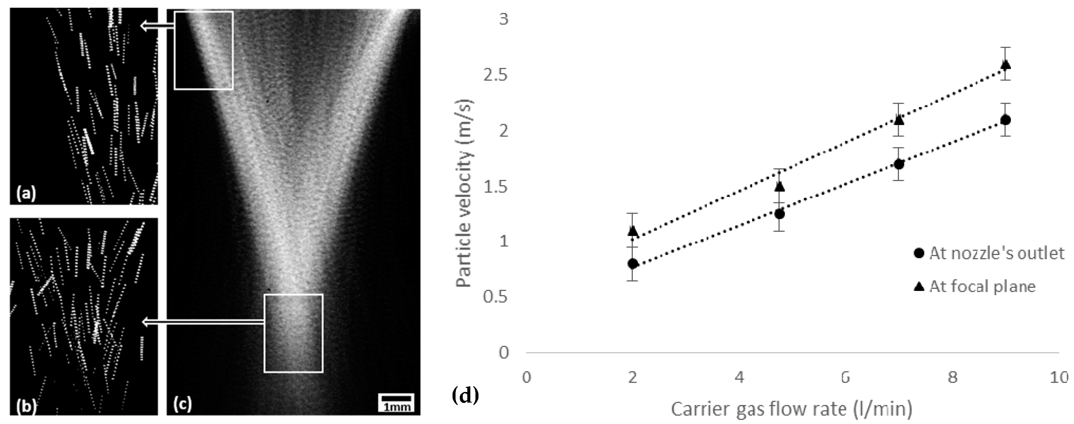
3.2.3. Analysis of the Particle Velocity

From the zoomed lateral views, the persistent trace of each particle can be obtained. The velocity of the powder particle (Vp) can then be expressed in terms of the leading and trailing point coordinates of the captured trace of a single particle (trace length) at a particular time instant over the shutter speed (Equation (2)). To clearly visualize the individual powder particle trace, observations were performed for a low mass flow rate of 4 g/min and calculations were made for a stack of 10 images.
V p = ( X 2 X 1 ) 2 + ( Z 2 Z 1 ) 2 t s h u t
where X2, Z2 are the coordinates of the leading point of the powder particle trace at a given time, and X1, Z1 are the coordinates of the trailing point of the same powder particle trace at the same time, and tshut = time shutter (s) of the camera. In the calculation of Equation (2), we have neglected the correcting factor due to the projection of the 3D particle flow, on the 2D camera sensor, because the mean projection angle θ being low (<10° in Figure 7), this correction should not exceed 1–2% (real 3D distance = measured distance/cos θ).
Figure 7 shows images of a powder stream captured on nozzle C, and corresponding particle velocities. Observations of Figure 7a,b highlight the different trace lengths, meaning that, besides the constant gas flow rate, particles travel at different velocities due to their size distribution [16] and to the multiple collisions with the nozzle walls during their trajectory [26]. Moreover, a tiny particle acceleration, from a mean velocity of 1.2 to 1.4 m/s (at 2 L/min carried gas flow rate), was observed between nozzle output and focal zone Figure 7d, revealing the continuous acceleration of the particles in the gas flow. An important point to note is that the mean particle velocity always stands below the carrier gas one (around 2 m/s on nozzle C for the same conditions). During the process, particles are set in motion by the carrier gas. According to their size and mass, they are supposed to reach the gas velocity after a particular travel time. However, due to the turbulent nature of the gas flow and the multiple collision of the particles with the nozzle walls during their trajectory, particles can acquire a different and slower velocity than the gas one. The difference between Vp and Vg can be link-related to the drag force effect (particle/gas friction), with the drag force FD = ½ ρ S Cx V2, with S as the particle section (m2), Cx the drag coefficient and V the relative particle/fluid speed (m/s) [27]. This effect is even more pronounced with nozzle A and B, for which the mean particle velocities never exceed 2.5 m/s, while the gas velocity field was, respectively, 10 and 3 times faster. Finally, similar to the results published by Kovaleva et al. [28] or Sergachev et al. [29], a limited number of particles were shown to accelerate under laser irradiation, due to severe heating, vaporization and corresponding recoil pressure. However, this effect was shown to be negligible in our case, with only a few detected particles enlightening, and subsequent high velocities.

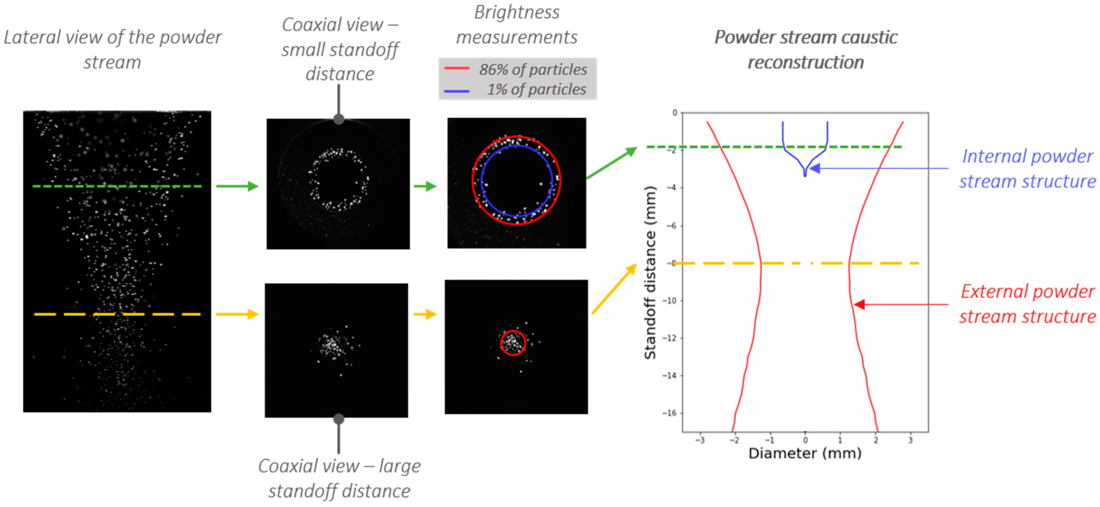
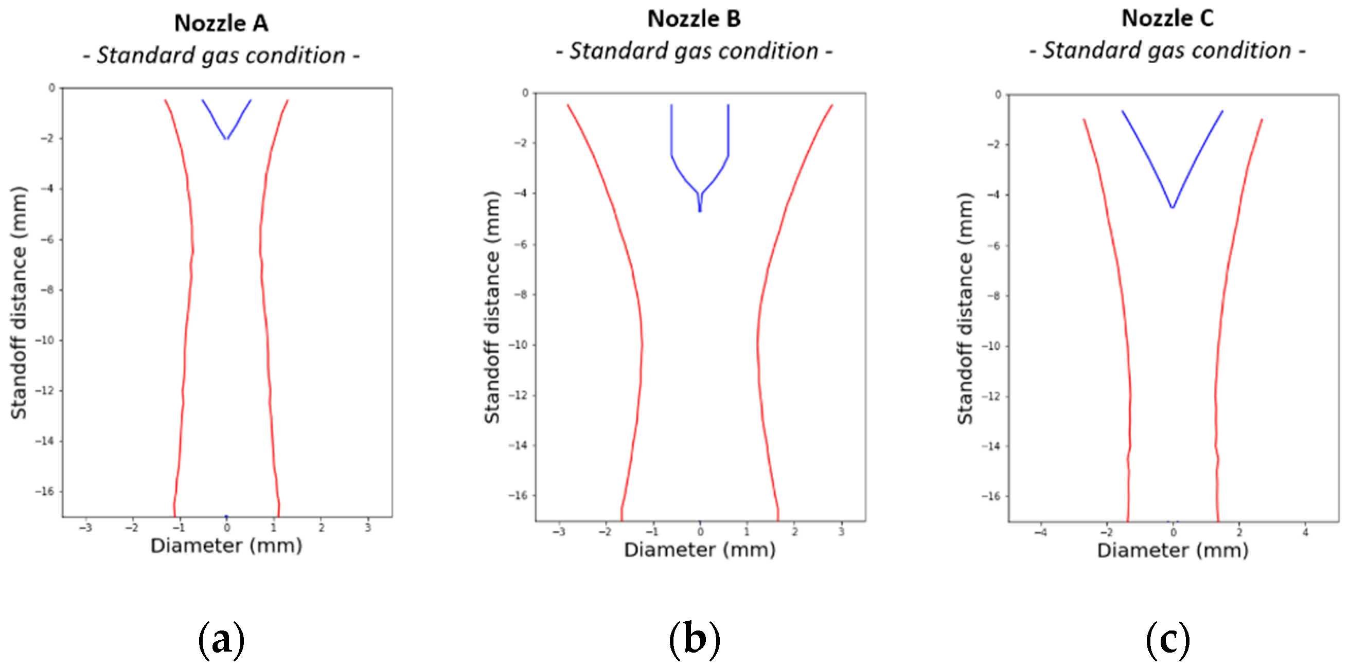
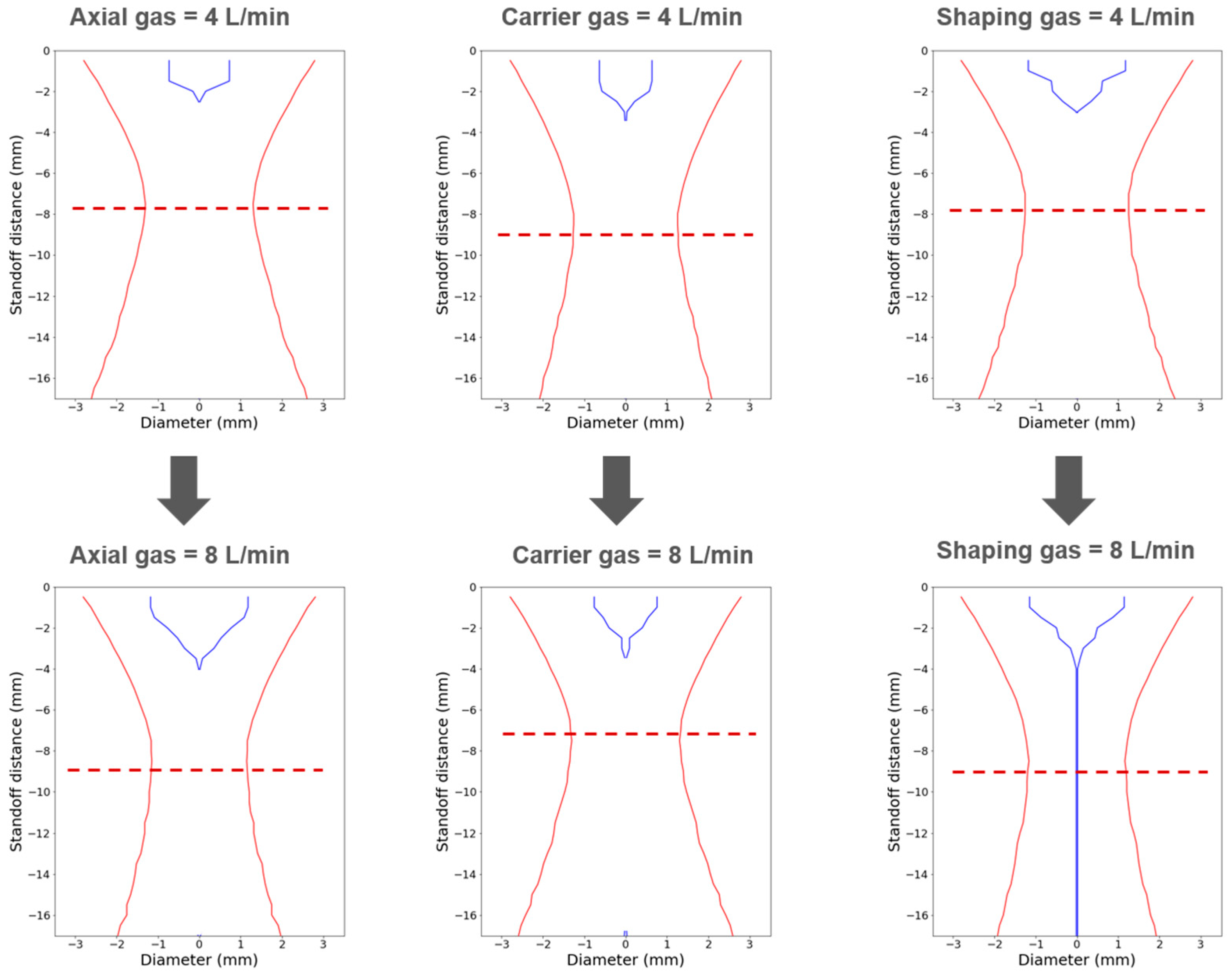
3.2.4. Powder Stream Caustic

To reduce the discrete nature of the recorded images, 100 images were stacked for each Z plan and a brightness threshold was used to remove light artefacts or spurious reflections from coaxial observation (Figure 8). To this point, it can be seen that the powder stream exhibits an annular shape at the nozzle’s exit and converges to a homogeneous stream for particular standoff distances. Compared to Nozzles A, Nozzles B and C’s results show a more non-homogenous shape below and above their focus plane (WD = 11 mm), with two (Nozzle B) or four (Nozzle C) brighter “parts”. This can be explained by the number of powder channel entrances of each nozzle and shows that the nozzle design, and probably the gas conditions, impact the mixing efficiency of the particles.
From the stacked images, we considered that the diameter of a circle encompassing 1% and 86% (1/e2) of the maximal luminosity of the lightened particles represented the inner and external diameter of a Gaussian powder jet, respectively. By conducting this analysis for all tested standoff distances (0.5 to 17 mm, ΔZ = 0.5 mm), a reconstruction of the powder stream caustic was performed (Figure 9). Experiments were completed for mass flow rates of 4, 6, 8 and 12 g/min, depending on the nozzle.
Figure 10 show the obtained caustic for each nozzle for their standard gas configuration (Table 2). The PFP is considered as the standoff distance leading to the narrowest stream diameter. Hence, results show that: (a) Nozzle A allows a nearly cylindrical powder stream, with a nearly constant diameter of 1.6 mm between 6 and 7.5 mm, (b) Nozzle B exhibits a 2.5 mm diameter stream at 11 mm working distance, and (c) Nozzle C generates a 2.6 mm diameter stream at a 12 mm standoff distance.
Figure 11 shows the powder stream behavior obtained for Nozzle B for variations in axial, carrier and shaping gas flow rates. Similar influences of axial, carrier and shaping gas flow were found for the three studied nozzles. The results show the following trends:
  • A 2 L/min increase in axial or shaping gas flow rate significantly pulls down the focus plane position of 1 and 1.5 mm, respectively;
  • A 4 L/min increase in the carrier gas cause a 1.5 mm rise in the convergence plane;
  • Axial and carrier gas have a very low impact on the powder stream diameter;
  • The activation of the shaping gas (only active on nozzles A and B) leads to a strong reduction in the powder stream diameter and dispersion and generates a more cylindrical stream in the convergence zone.
The influence of the powder flow rate Dm is exposed for two gas conditions in Figure 12a for Nozzle A and in Figure 12b for Nozzle B. For all tested conditions, Dm does not impact the focus plane position. However, for high Dm values (≥12 g/min), Nozzle B’s stream diameter increased from 2 to 2.6 mm at the PFP. This expansion of the powder stream for high Dm can be explained by the increase in the particle number, resulting in more particle collisions and a higher dispersion of the stream. Equivalent trends are shown with Nozzle A above 8 g/min, with a focus diameter increase of 0.6 mm, but only when a low axial gas is used (DAG = 1 L/min).
In sum, these results highlight the influence of the gas flow rate on the focus plane position whereas the powder stream diameter seems to be mostly influenced by the powder flow rate and the nozzle geometry.

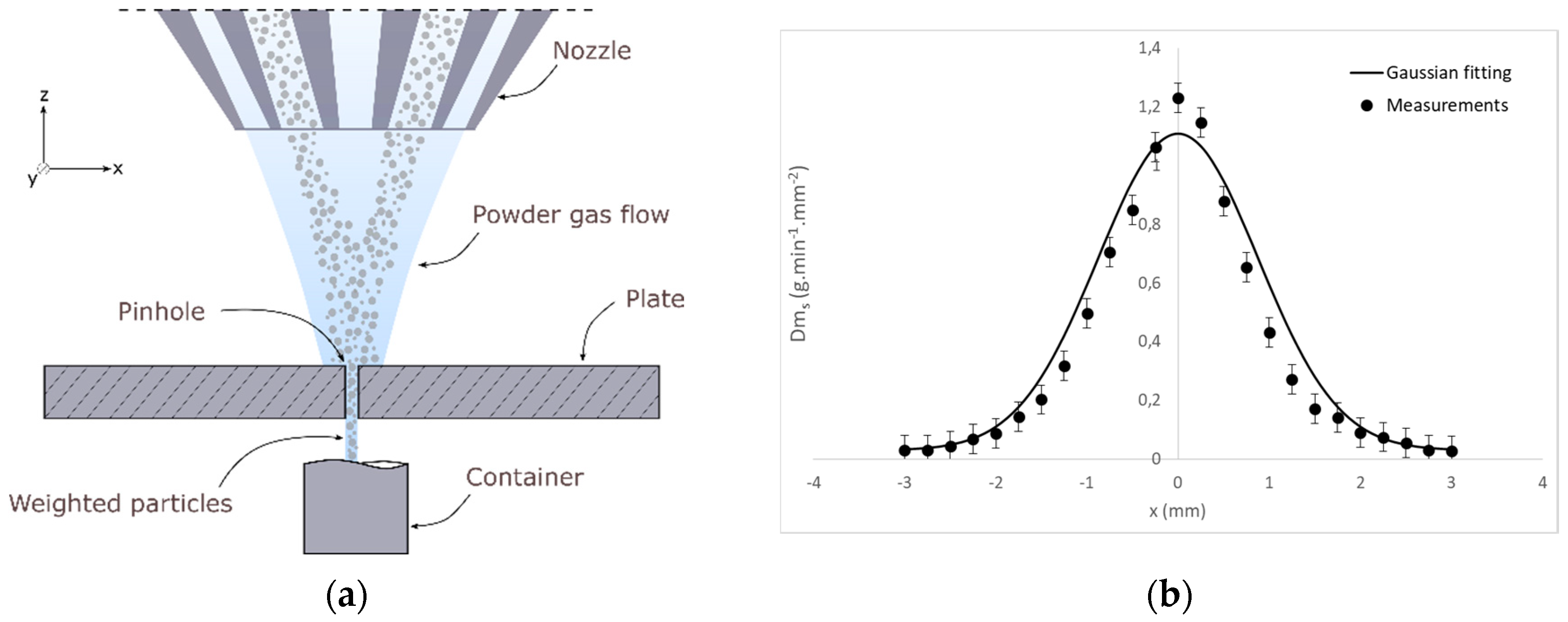
3.2.5. Powder Flow Density

Another important parameter of the powder stream is its particle surface density Dms (g·mm2·s−1) on a particular XY plan. This parameter can be measured using a plate with a circular pinhole (0.4 mm), disposed at a known standoff distance below the nozzle outlet (Figure 13a). By weighting the fraction of the particles able to go through the pinhole (mph) for multiple static position of the nozzle along the X axis (Δx = 0.25 mm), the local powder flow density can be calculated by the following expression
D m s = m p h ( g ) d t ( s ) * S p h ( m m 2 )
with Sph the pinhole area and dt the measurement time at each point. During this experiment, the nozzle stays in a static position during dt = 5 min for each measurement point to obtain enough particles to weigh.
Figure 13b shows the obtained curve. By numerically integrating the surface mass flow (the area under the curve), only 80% of the total powder flow rate is found. This 20% particle loss can be explained by fluctuations of the powder flow, particles rebounds on the plate or by the gas flow disturbance around the pinhole during the experiment. Considering this, the total flow rate used for the rest of this part is the numerically obtained one and not the 6 g/min programmed in the machine. Then, given the Gaussian-like distribution profile of the particle surface density curve, a Gaussian fitting was proposed according to the following equation
C ( r ) = ln ( 1 1 p ) π   ·   D m n r j e t 2   ·   e ln ( 1 1 p ) ·   r 2 r j e t 2
with Dmn the total powder flow rate numerically found (80% of 6 g/min); rjet (mm) the powder stream radius, defined as the radius which concentrate p% of the total powder flow rate; and p (%) the percentage of Dm where rjet is measured, chosen at 86% (1/e2).
Despite the top hat distribution of the gas velocity field, results show that the proposed Gaussian form allows a fairly good approximation of the mass flow distribution in the focal plane, with an error of 0.051 g·min−1·mm−2 on average, 10% of the average surface mass flow. As shown by Eisenbarth et al. [12], this circular Gaussian approximation is only valid for a measurement around the powder stream’s PFP, previous optical measurements are then needed to efficiently and quickly reveal the PFP position. Therefore, this weighing method can be used as a complementary experimental technic for the powder stream analysis.

4. Modeling of the Jet Flow

The numerical modeling of the jet flow from the deposit nozzles was carried out with COMSOL Multiphysics 5.3a software. A two-phase flow was considered, composed of a continuous gas phase and a discrete particle phase. The jet flow is solved by modeling the primary gas phase and then by incorporating the secondary particle phase. Such a Euler–Lagrange model is valid here, since the discrete particle phase volume is less than 10% of the total volume. Due to the conical shape of the three studied nozzle designs, a 2D axisymmetric model was used. With this first hypothesis, we considered a homogenous and axisymmetric particle flow, which is not the exact reality, as shown in Figure 3. However, this assumption allows an optimized computational time and still provides a good representation of the jet. Based on this 2D model, the scheme of the computational domain includes the internal geometry of the nozzle channels and a cylindrical computation area (Φ = 30 mm; L = 30 mm) allowing to visualize the gas flow behavior below the nozzle.

4.1. Modeling of the Primary Gas Phase

For the modeling of the gas phase, an inert atmosphere was assumed, meaning that the gas flowing inside the nozzles and the external atmosphere is argon. This assumption is easier to implement than a mixture of two gases (inert and air-based) and is adapted to many real deposit cases. The gas is set with pure argon properties (Table 1) and was supposed as Newtonian and incompressible, due to the low gas pressure (< 0.3 MPa) at the nozzle’s outlets.

4.1.1. Governing Equations

As the Reynolds number of the flows is quite high—at least 1000, according to the nozzle geometry—a turbulent model must be considered. Moreover, to reduce the computation type and assuming that the unsteadiness in the flow and the flow itself can be treated separately, the Reynolds Average Navier– Stokes (RANS) models was used. Therefore, for an incompressible flow, the turbulent model can be described by the two equations below [6]
Conservation of mass:
ρ · ( u ) = 0
Conservation of momentum (Navier-Stokes):
ρ u t + ρ ( u · ) u = · [ p I + μ   ( u + u T ) ]  
where u is the mean velocity vector, p is the pressure, ρ is the gas density and μ is the dynamic viscosity of the gas.
At this point, mean velocity and pressure values can only be solved with these equations if the Reynolds stress tensor can be derived in some way. Therefore, the temporal and spatial evolution of the gas flow needs to be specified by new equations in a time average manner. Corresponding formulations can be provided by diverse turbulence models, among which the most commonly used is a two-equation model known as the k-ϵ. In this case, the turbulence field is characterized by the kinetic energy κ and the viscous dissipation rate of the turbulent kinetic energy ε. Then, two transport equations can be obtained from the Navier-Stokes as follows [6]
Conservation of the kinetic energy of turbulence:
x j ( ρ u ¯ j k ) = x j ( μ t σ k k x j ) + G k + G b ρ ε
Conservation of the dissipation of kinetic energy of turbulence:
x j ( ρ u ¯ j ε ) = y x j   (   μ t σ ε ε x j ) + C 1   ε k   (   G k + G b   ) C 2   ρ   ε 2 k
G k = μ t   u ¯ i x j   ( u ¯ i x j + u ¯ j x i )
G b = g i   μ t ρ   P r t   ρ x i
μ t = ρ   C μ   k 2 ε
where u is the gas velocity vector, i,j = r,z axes, μ = μ 0 + μ t   (with μ 0 the molecular/laminar viscosity, μ t the turbulent viscosity from Kolmogorov–Prandlt) and g i is the gravitational acceleration. C 1 ,   C 2 ,   σ ε ,   σ k   a n d   C μ are empirical constant optimized by the years as follows: C 1 = 1.44, C 2 = 1.92, σ ε = 1.3, σ k = 1.0, C μ = 0.09 [COMSOL 5.3a]. G k and G b represent, respectively, the rate of production of kinetic energy and the generation of turbulence, P r t is the turbulent Prandtl number of energy.

4.1.2. Boundary Settings

To numerically solve the turbulent Navier–Stokes equation system, the initial pressure was set to P0 = 1.105 Pa and the initial temperature T0 = 293 K. As for the gas initial condition, the flow rates of each gas flow were pre-set at the channels input of each nozzle. A standard no-slip condition was assigned to the nozzle walls and the outlet of the computational domain was treated as a pressure outlet of 1.105 Pa, and a “disappearing” condition was used. The calculation was then performed to find a time-average stationary solution.

4.2. Modelling of the Secondary Particle Phase

The particle discrete phase is calculated with a particle tracing model and by solving the particles kinematics equations. The trajectory of the particle flow is solved by integrating the force balance on each particle in a Lagrange reference frame. The particles dynamics is driven by the gas flow drag force, and the force equation balances the particle inertia and the drag force acting on the particle. A Harder–Levenspiel drag law was set [30] and the force balance equation is as below
d u p d t = m p τ p   [ u u p ]
τ p = 4   ρ p   d p 2   3   μ   C D   R e  
R e = ρ p   D p   | u p u g | μ
with u p , d p , m p and ρ p the velocity, diameter, mass and density of a single particle, respectively; Re is the Reynolds number.
For boundary conditions, specific numbers of particles are released every 000.1 s to obtain the needed feed rate (36 particles for Dm = 6 g/min, for example) and a stationary solution was obtain for a computation of 0.2 s. All particles were considered spherical and a Gaussian size distribution was set according to the experimental data. The inlet distribution density of the particles was set to be proportional to the gas velocity. A “disappear” wall was displayed for each boundary of the external area, except for the axisymmetric axis, where an elastic rebound was considered. Collisions between particles were neglected due to their low volume fraction (< 10%) and no heat transfer between gas and particles was considered so that all particles remained solid during their time-of-flight. Finally, inelastic rebounds of particles on the nozzle walls were considered as a 10% loss of the incident particle velocity during rebound [20].

4.3. Numerical Results and Comparison with Experiements
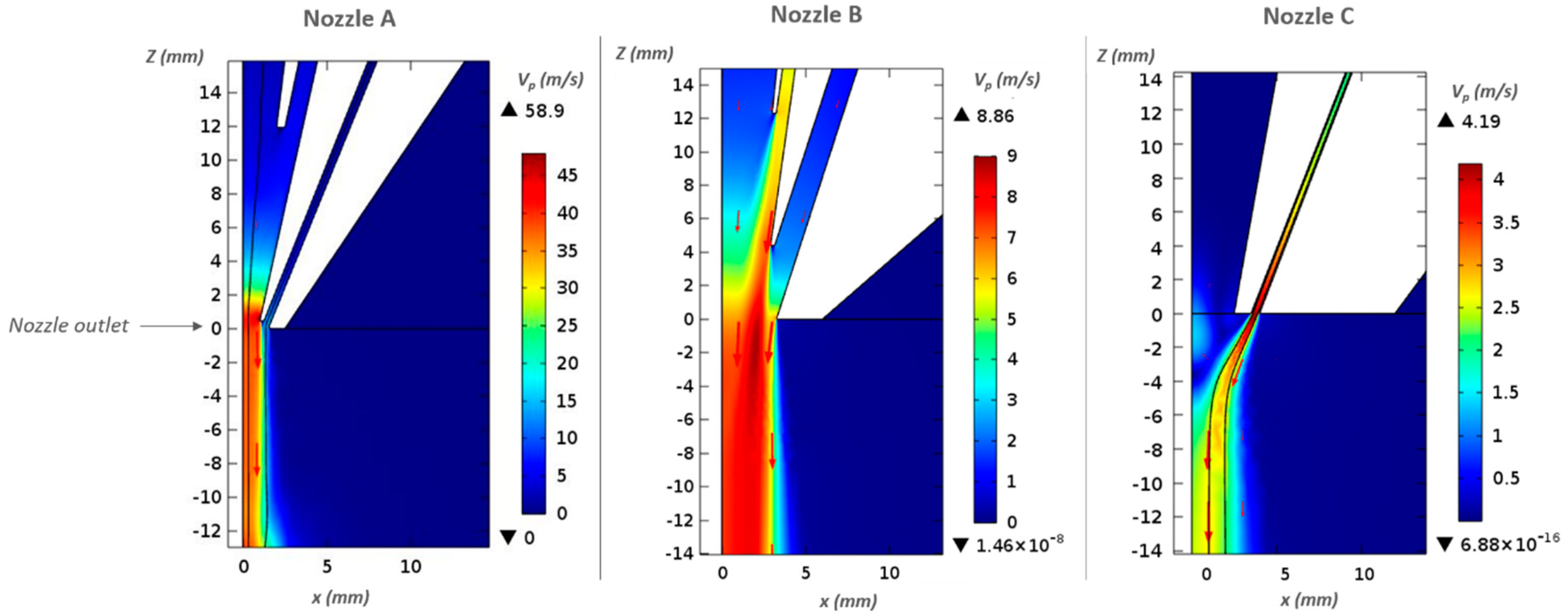
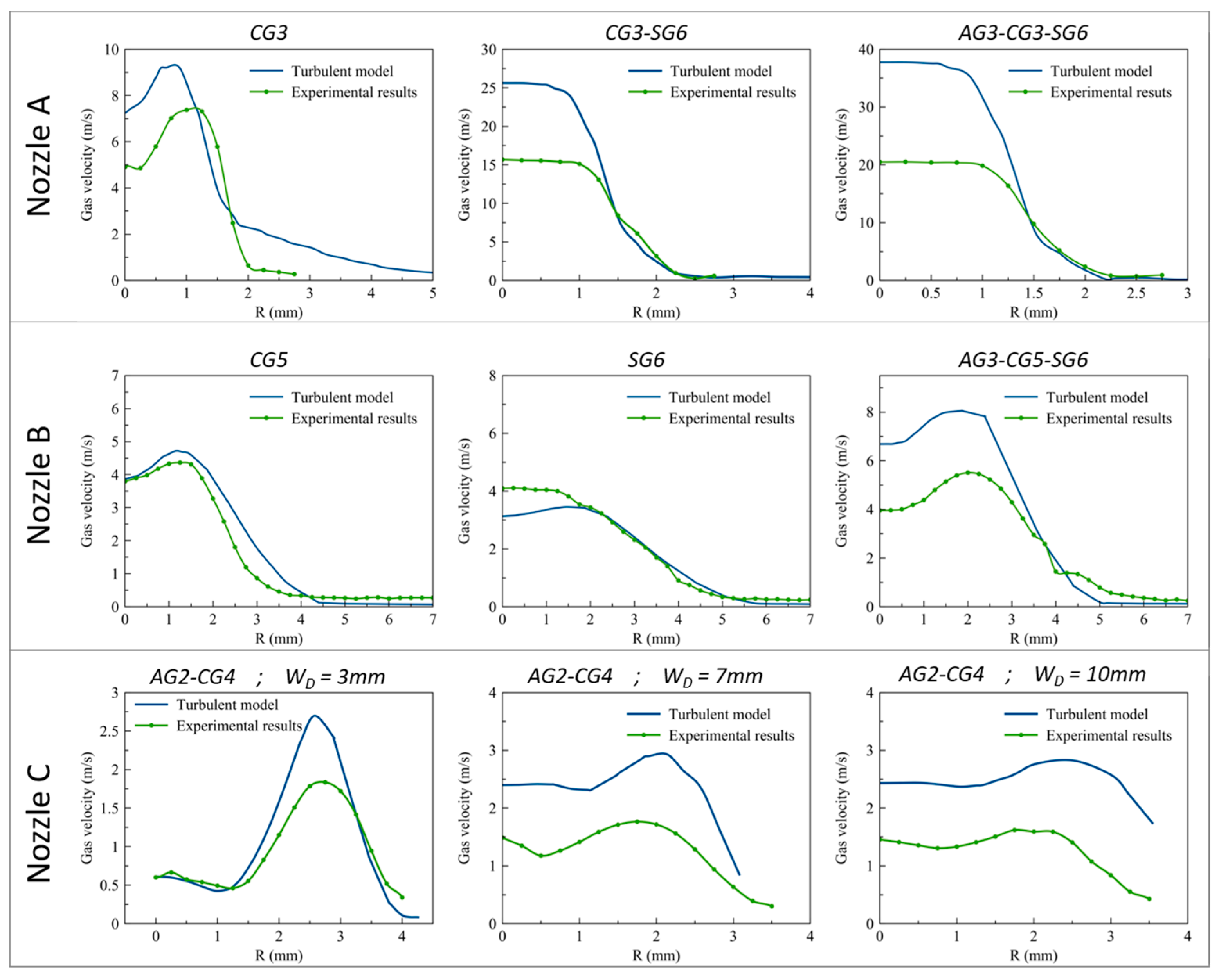
4.3.1. Gas Velocity

For standard set of gas inflow rate (Table 2), Figure 14 shows the gas flow velocity field inside the channels of nozzles A, B and C and in their external area. In each case, the gas flow undergoes a significant acceleration, caused by a combination of the different fluxes and by the convergent shape of nozzle channels, and reaches a maximum velocity at the nozzle outlet. Nozzle C’s velocity field seems to be mostly governed by the carried gas flow, because of its much finer channel passage and to the low axial gas flow input (2 L/min). Gas velocities reach a 59 m/s for nozzle A, and 9 and 4 m/s for nozzles B and C, respectively. From this point, nozzle C’s gas stream decelerates in the inert atmosphere and reaches 2.5 m/s around its standard standoff distance (WD = 10 mm). Nozzle A’s gas flow follows the same trend, and decelerate from the exit to reach Vgas = 38 m/s at WD = 3.5 mm. On the contrary, Nozzle B streams do not decelerate as fast and maintain rather constant mean velocity of 8 m/s on a range of standoff distances. This can be explained by its wider nozzle exit dimension, which generate less acceleration and then a slower deceleration.
Comparison of the measured and simulated gas velocity field along R (radius) are shown on Figure 15 for different gas conditions or standoff distances. First, we can see that, for each nozzle, both experimental and numerical results agreed on the gas stream diameter as well as on the shape of the gas velocity distribution: annular when the carrier gas only is activated or is predominant; top hat for the other conditions. Nozzles B and C exhibit a better agreement when only one or two gas channels are activated, and show an error up to 30% of the measured velocity in all cases. This gap between experimental and numerical results is greater with Nozzle A: errors of 20%, 38% and 54% are estimated when one, two and three gas channels are activated, respectively. It seems that the turbulent numerical model always overestimates the gas velocity field and that the gap with experimental results becomes greater when gas velocity is higher than 3–4 m/s. Differences between experimental and numerical results can be explained by:
  • The atmosphere conditions below the nozzle: numerical work considered an inert argon atmosphere while an air-based area was used for the experimental investigations. Visualization of the gas structure by Nagulin et al. [17], revealed the formation of instabilities between the injected inert gas jet and an air-based atmosphere. These instabilities become greater with an increase in the gas flow and may disturb the gas stream and slow it down. Then, when only one gas channel is activated, a simpler and slower flow with few instabilities appears, which seems to be quite well predicted by C 1 ,   C 2 ,   σ ε ,   σ k   a n d   C μ empirical parameters. However, a more complex and turbulent flow appears when two or three gas channels are simultaneously activated. The previous empirical parameters might then not be perfectly adapted for such a case.
  • Gaps obtained between experimental and numerical results could also be explained by an insufficient calibration of the Pitot tube, which was only calibrated for air-based flows.
  • The Pitot size can also impact the measurement and give a more average velocity of the velocity field below the nozzles. Indeed, analytical calculations (Equation (15)) were performed to estimate the gas flow velocity at the nozzle exit and compared to average velocity results obtained at usual standoff distances of Nozzles A and B for multiple gas conditions (Table 4). This shows close results between analytical and experimental measurements when only one gas channel is activated. However, analytical results (Table 4 and Equation (15)) seem to be closer to numerical ones when two or three gas channels are opened during the process. Pitot tube measurement might then underestimate the real gas velocity field.
    V g = D g   ( m 3 · s 1 ) S   ( m 2 ) ,   with   S   the   exit   surface   of   the   nozzle

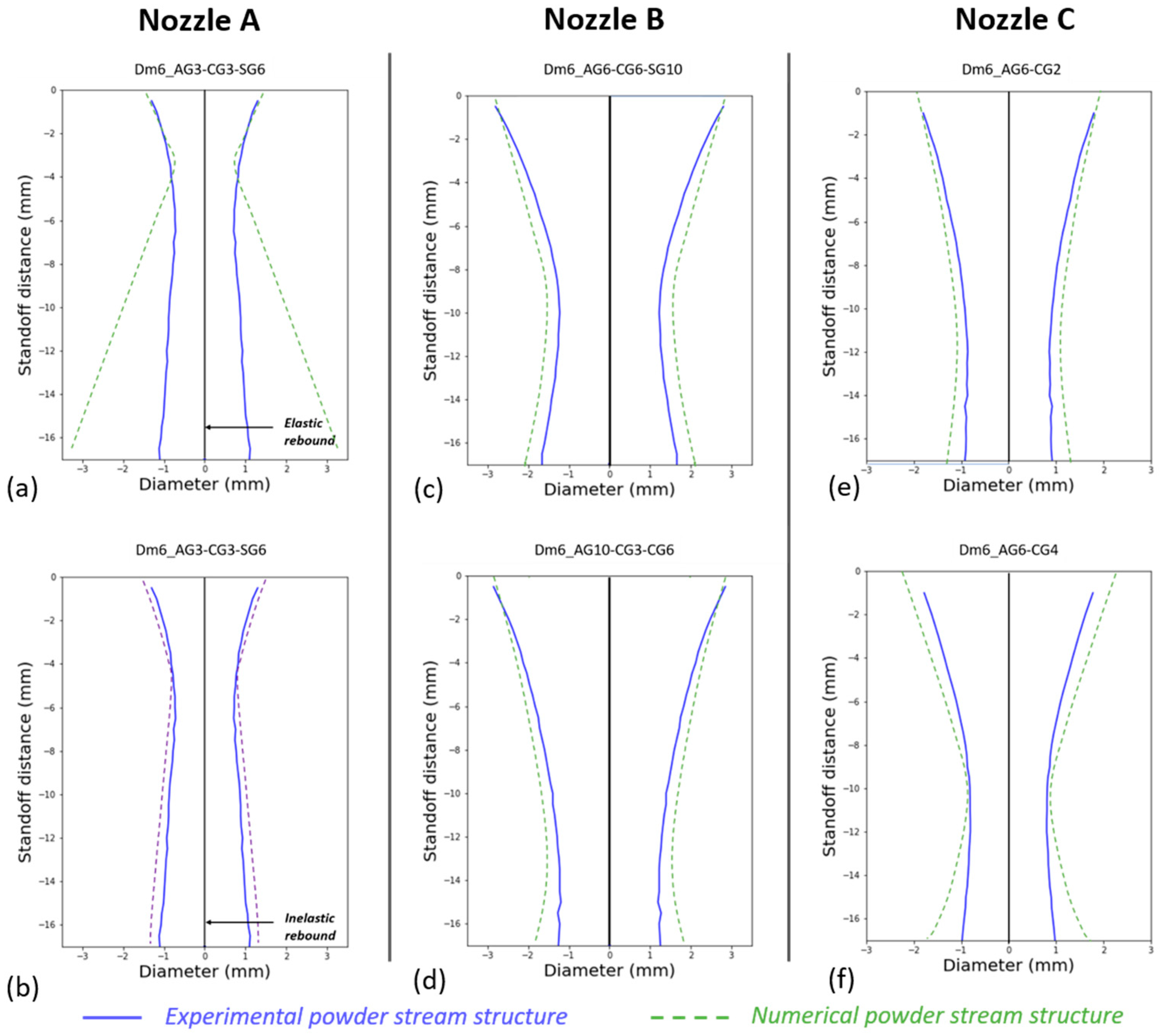
4.3.2. Powder Stream

Now focusing on powder particle flow, Figure 16 shows the continuous acceleration of the powder inside the nozzle channels. As shown by [31], the powder jet can be divided into three distinct regimes: converging, focal and diverging zones, with the area from the nozzle exit to the lower plane considered. Compared to the gas behavior, particles continue to accelerate below the nozzle outlet and reach their maximum value after their focal position. Except for Nozzle A, the maximum particle velocity reaches approximately 0.3 times the gas velocity. Moreover, despite the great gas velocity obtained with Nozzle A simulations, the particles velocities do not exceed 1 m/s for all tested gas configuration due to their inertia.
Figure 17 shows the comparison of the experimental (dotted line) and numerical (solid line) powder stream caustic for the three nozzles, for one or two gas conditions. Gas conditions were selected to obtain sufficiently different caustics to ensure the model validity. Nozzle B’s results shows a good agreement between experimental and numerical powder stream caustics for both gas conditions (Figure 17c,d). A ± 0.5 mm difference is measured between the two caustics for the focal plane position. However, the diameter of the convergent part of the stream seems to be overestimated by the simulation. This can be explained by the non-consideration of the particles’ collisions with each other, which deviates their trajectories and slows them down. The same results were found with nozzle C (Figure 17f).
Nozzle A’s comparison results (Figure 17a) show very dissimilar jet structures. The experimental powder stream follows a cylindrical like shape, while a more convergent stream is numerically obtained. For this particular nozzle simulation, the powder stream seems to be mainly governed by the powder elastic rebound on the axis of symmetry than by gas conditions. This elastic rebound allows the observation of the divergent part of the stream but might not be accurate since it does not consider the multiple particle collisions around the focal plane, which impact the trajectories and velocities of each particles. This phenomenon is particularly notable with Nozzle A because of its thinner powder stream: for an identical number of particles injected by the three nozzles (same Dm), Nozzle A shows a thinner diameter; then, collision between particles is more likely to append. Similar observations could appear with Nozzles B and C for very high powder flow rates. Considering this, new simulations were performed with an inelastic rebound on the axis of symmetry of nozzle A with 30% of velocity loss after the impact [20]. Results show a much better agreement with experimental results, even if the stream diameter at the focal plane is still slightly over-estimated by numerical results (Figure 7b). Therefore, the simulation seems to be dependent on the particle concentration and the particle collision boundary condition. One way to enhance the model could be to link the particle rebound factor with the particle concentration: the rebound would stay elastic (α = 1) for a small particle concentration and would become inelastic (α < 1) with its increase.

5. Conclusions

In this paper, four experimental techniques were investigated to analyze the characteristics of the gas and powder streams under multiple gas and powder flow rates conditions for three coaxial LMD nozzle designs. 2D axisymmetric turbulent models were performed on the basis of the Euler–Lagrange theory to compare with the experimental results properties of the streams, such as its particle velocity, surface density, diameter and focal plane position.
(1)
3D measurements of the gas velocity fields were performed by moving the nozzles below a Pitot tube. The measurements highlighted a “top hat” like distribution of the velocity field as long as the carrier gas flow is not the only one activated;
(2)
Coaxial observation of the powder stream and luminosity measurements gave a rapid and effective way to obtain the 3D powder stream structure. Results showed that an increase in the axial and shaping gas flow rate significantly pulls down the focus plane position, while an increase in the carrier gas one raises it up. The diameter of the powder stream is, however, mainly governed by the nozzle geometry and shaping gas flow rate;
(3)
Spatial powder flow measurements were performed by moving the nozzle above a pinhole with a specific standoff distance and weighing the trapped particles. On the contrary to the top hat gas distribution, the powder surface density is well fitted with a Gaussian distribution (error of 10%);
(4)
Comparisons between numerical and experimental results show that particle rebound conditions have a great impact on the model and should be linked or proportional to the particle concentration to correctly describe the powder stream structure, especially for nozzles with small exit diameters. Considering this, the model can be useful to understand the influence of other process parameters (such as gas, particle or nozzles parameters, for example) and to help new nozzle designs to enhance the effectiveness of the process.

Author Contributions

Investigation, E.F., C.G. and J.G.; Methodology, C.G. and D.C.; Project administration, P.P.; Writing—original draft, E.F.; Writing—review and editing E.F., M.D., C.C., G.M., C.G. and P.P. All authors have read and agreed to the published version of the manuscript.

Funding

This research received no external funding

Conflicts of Interest

The authors declare no conflict of interest.

References

  1. Kelbassa, I.; Albus, P.; Dietrich, J.; Wilkes, J. Manufacture and repair of aero engine components using laser technology. In Proceedings of the 3rd Pacific International Conference on Applications of Lasers and Optics, PICALO 2008-Conference Proceedings, Beijing, China, 16–18 April 2008; pp. 208–213. [Google Scholar]
  2. Yu, J.H.; Choi, Y.S.; Shim, D.S.; Park, S.H. Repairing casting part using laser assisted additive metal-layer deposition and its mechanical properties. Opt. Laser Technol. 2018, 106, 87–93. [Google Scholar] [CrossRef]
  3. Schneider-Maunoury, C. Application de L’injection Differentielle au Procédé de Fabrication Additive DED-CLAD Pour la Réalisation D’alliages de Titane à Gradients de Compositions Chimiques; Université de Lorraine: Metz, France, 2020. [Google Scholar]
  4. Xue, L.; Islam, M.U. Laser Consolidation—A Novel One-Step Manufacturing Process for Making Net-Shape Functional Components; National Research Council of Canada Ottawa (Ontario): Ottawa, ON, Canada, 2006. [Google Scholar]
  5. Liu, R.; Wang, Z.; Sparks, T.; Liou, F.; Newkirk, J. Aerospace applications of laser additive manufacturing. In Laser Additive Manufacturing: Materials, Design, Technologies, and Applications; Elsevier Inc.: Amsterdam, The Netherlands, 2016; pp. 351–371. [Google Scholar]
  6. Zekovic, S.; Dwivedi, R.; Kovacevic, R. Numerical simulation and experimental investigation of gas-powder flow from radially symmetrical nozzles in laser-based direct metal deposition. Int. J. Mach. Tools Manuf. 2007, 47, 112–113. [Google Scholar] [CrossRef]
  7. Zhu, G.; Li, D.; Zhang, A.; Tang, Y. Numerical simulation of metallic powder flow in a coaxial nozzle in laser direct metal deposition. Opt. Laser Technol. 2011, 43, 106–113. [Google Scholar] [CrossRef]
  8. Takemura, S.; Koike, R.; Kakinuma, Y.; Sato, Y.; Oda, Y. Design of powder nozzle for high resource efficiency in directed energy deposition based on computational fluid dynamics simulation. Int. J. Adv. Manuf. Technol. 2019, 105, 4107–4121. [Google Scholar] [CrossRef]
  9. Wu, J.; Zhao, P.; Wei, H.; Lin, Q.; Zhang, Y. Development of powder distribution model of discontinuous coaxial powder stream in laser direct metal deposition. Powder Technol. 2018, 340, 449–458. [Google Scholar] [CrossRef]
  10. Mezari, R. Etude du Contrôle de Procédé de Projection Laser pour la Fabrication Additive: Instrumentation, Identification et Commandes; Ecole Nationale Supérieure D’arts et Métiers—ENSAM: Paris, France, 2014. [Google Scholar]
  11. Gharbi, M. Etats de Surface de Pièces Métalliques Obtenues en Fabrication Directe par Projection Laser (FDPL): Compréhension Physique et Voies D’amélioration; Ecole Nationale Supérieure D’arts et Métiers: Paris, France, 2016. [Google Scholar]
  12. Eisenbarth, D.; Esteves, P.M.B.; Wirth, F.; Wegener, K. Spatial powder flow measurement and efficiency prediction for laser direct metal deposition. Surf. Coat. Technol. 2019, 362, 397–408. [Google Scholar] [CrossRef]
  13. Liu, Z.; Zhang, H.C.; Peng, S.; Kim, H.; Du, D.; Cong, W. Analytical modeling and experimental validation of powder stream distribution during direct energy deposition. Addit. Manuf. 2019, 105, 4107–4121. [Google Scholar] [CrossRef]
  14. Tabernero, I.; Lamikiz, A.; Ukar, E.; de Lacalle, L.N.L.; Angulo, C.; Urbikain, G. Numerical simulation and experimental validation of powder flux distribution in coaxial laser cladding. J. Mater. Process. Technol. 2010, 210, 2125–2134. [Google Scholar] [CrossRef]
  15. Cortina, M.; Arrizubieta, J.I.; Ruiz, J.E.; Ukar, E. Latest developments in industrial Hybrid Machine Tools that combine additive and subtractive operations. Materials 2018, 11, 2583. [Google Scholar] [CrossRef] [Green Version]
  16. Balu, P.; Leggett, P.; Kovacevic, R. Parametric study on a coaxial multi-material powder flow in laser-based powder deposition process. J. Mater. Process. Technol. 2012, 212, 1598–1610. [Google Scholar] [CrossRef]
  17. Nagulin, K.Y.; Iskhakov, F.R.; Shpilev, A.I.; Gilmutdinov, A.K. Optical diagnostics and optimization of the gas-powder flow in the nozzles for laser cladding. Opt. Laser Technol. 2018, 108, 310–320. [Google Scholar] [CrossRef]
  18. Koike, R.; Takemura, S.; Kakinuma, Y.; Kondo, M. Enhancement of powder supply efficiency in directed energy deposition based on gas-solid multiphase-flow simulation. Procedia CIRP 2018, 78, 133–137. [Google Scholar] [CrossRef]
  19. Arrizubieta, J.L.; Tabernero, I.; Ruiz, J.E.; Lamikiz, A.; Martinez, S.; Ukar, E. Continuous coaxial nozzle design for LMD based on numerical simulation. Phys. Procedia 2014, 56, 429–438. [Google Scholar] [CrossRef] [Green Version]
  20. Kovalev, O.B.; Kovaleva, I.O.; Smurov, I.Y. Numerical investigation of gas-disperse jet flows created by coaxial nozzles during the laser direct material deposition. J. Mater. Process. Technol. 2017, 249, 118–127. [Google Scholar] [CrossRef]
  21. Zhong, C.; Pirch, N.; Gasser, A.; Poprawe, R.; Schleifenbaum, J. The Influence of the Powder Stream on High-Deposition-Rate Laser Metal Deposition with Inconel 718. Metals 2017, 7, 443. [Google Scholar] [CrossRef] [Green Version]
  22. Spelay, R.B.; Adane, F.; Sanders, R.S.; Sumner, R.J.; Gillies, R.G. The effect of low Reynolds number fl ows on pitot tube measurements. Flow Meas. Instrum. 2015, 45, 247–254. [Google Scholar] [CrossRef]
  23. Chevula, S.; Sanz-Andres, Á.; Franchini, S. Estimation of the correction term of pitot tube measurements in unsteady (gusty) flows. Flow Meas. Instrum. 2015, 46, 179–188. [Google Scholar] [CrossRef]
  24. Vinod, V.; Chandran, T.; Padmakumar, G.; Rajan, K.K. Calibration of an averaging pitot tube by numerical simulations. Flow Meas. Instrum. 2012, 24, 26–28. [Google Scholar] [CrossRef]
  25. Boetcher, S.K.S.; Sparrow, E.M. Limitations of the standard Bernoulli equation method for evaluating Pitot/impact tube data. Int. J. Heat Mass Transf. 2007, 50, 782–788. [Google Scholar] [CrossRef]
  26. Kovalev, O.B.; Zaitsev, A.V.; Novichenko, D.; Smurov, I. Theoretical and experimental investigation of gas flows, powder transport and heating in coaxial laser direct metal deposition (DMD) process. J. Therm. Spray Technol. 2011, 20, 465–478. [Google Scholar] [CrossRef]
  27. Mailliat, A. Les Milieux Aérosols et Leurs Représentations; EDP Sciences: Les Ulis, France, 2010. [Google Scholar]
  28. Kovaleva, I.O.; Kovalev, O.B. Simulation of the acceleration mechanism by light-propulsion for the powder particles at laser direct material deposition. Opt. Laser Technol. 2012, 44, 714–725. [Google Scholar] [CrossRef]
  29. Sergachev, D.V.; Kovalev, O.B.; Grachev, G.N.; Smirnov, A.L.; Pinaev, P.A. Diagnostics of powder particle parameters under laser radiation in direct material deposition. Opt. Laser Technol. 2020, 121, 105842. [Google Scholar] [CrossRef]
  30. Morville, S. Modélisation Multiphysique du Procédé de Fabrication Rapide par Projection Laser en vue D’améliorer L’état de Surface Final; Université de Bretagne-Sud: Lorient, France, 2012. [Google Scholar]
  31. Wen, S.Y.; Shin, Y.C.; Murthy, J.Y.; Sojka, P.E. Modeling of coaxial powder flow for the laser direct deposition process. Int. J. Heat Mass Transf. 2009, 52, 5867–5877. [Google Scholar] [CrossRef]
Figure 1. Basic principle of the Laser Metal Deposition (LMD) process.
Metals 10 00667 g001
Figure 2. Cross-sections of the three nozzles A, B and C.
Metals 10 00667 g002
Figure 3. (a) Pitot measurement setup; gas velocity maps of the gas stream for a working distance of: 1 and 3 mm below nozzle A (AG3-CG3-SG6) (b); 11 and 13mm below nozzle B (AG6-CG5-SG3) (c); 1, 7, 9 and 11 mm below nozzle C’s tips (AG2-CG4) (d).
Metals 10 00667 g003
Figure 4. Velocity field distribution Vgas = f(x) along the X axis for multiple: (a) carrier (CG5 = 5 L/min carrier gas) and (b) shaping gas (SG6 = 6 L/min shaping gas) flow rates (nozzle B).
Metals 10 00667 g004
Figure 5. Velocity field distribution Vgas = f(x) along the X axis for multiple: (a) carrier and (b) shaping gas flow rate with nozzle A; (c) influence of gas channels activation on the velocity field distribution (nozzle A).
Metals 10 00667 g005
Figure 6. (a) Schematic of the combined (lateral + coaxial) observation of the powder stream; (b) Experimental setup.
Metals 10 00667 g006
Figure 7. Lateral observation of the powder stream: (a) Up-left zoomed view; (b) zoom around the PFP; (c) complete view of the stream, (d) influence of carrier gas flow rate on particle’s velocity (all graphs correspond to nozzle C).
Metals 10 00667 g007
Figure 8. Coaxial views of the powder stream for nozzles A, B and C and for multiple working distances (WD) below the nozzle’s outlet.
Metals 10 00667 g008
Figure 9. Powder stream caustic analysis from coaxial observation (Nozzle B).
Metals 10 00667 g009
Figure 10. Powder stream caustic for Nozzles A (a), B (b) and C (c) with standard parameters.
Metals 10 00667 g010
Figure 11. Influence of gas axial (left), carrier (middle) and shaping (right) gas flow rate on nozzle B’s powder jet structure and its focus plane (dotted line).
Metals 10 00667 g011
Figure 12. Influence of Dm on the powder stream structure for particular gas conditions with (a) Nozzle A and (b) Nozzle B.
Metals 10 00667 g012
Figure 13. (a) Schematic of the experiment; (b) Particle surface density results of Nozzle C at its focal plane (Wd = 12 mm) for Dm = 6 g/min.
Metals 10 00667 g013
Figure 14. Simulated argon flow velocities for nozzles A (left), B (middle) and C (right).
Metals 10 00667 g014
Figure 15. Comparison of the velocity field experimentally obtained (dotted line) with numerical (solid line) results for nozzles A, B and C.
Metals 10 00667 g015
Figure 16. Particle trajectory for nozzle A (left), B (middle) and C (right).
Metals 10 00667 g016
Figure 17. Comparison between experimental (solid blue lines) and numerical (dotted green lines) powder stream structures obtained for Nozzle A with elastic (a) and inelastic rebound (b) at the axis of symmetry for AG3-CG3-SG6; Nozzle B for AG6-CG6-SG10 (c) and AG10-CG3-SG6 (d); Nozzle C for AG6-CG2 (e) and AG6-CG4 (f).
Metals 10 00667 g017
Table 1. Argon properties at room temperature and nozzle parameters.
Density (kg·m−3)Dynamic Viscosity (Pa·s)
1.632.26 × 10−5
Table 2. Nozzles A, B and C standard parameters and external part’s exit diameters.
NozzleDAG (L/min)DCG (L/min)DSG (L/min)WD (mm)Exit Diameter (mm)
A3363.53
B653136.5
C24/107
Table 3. Experimental gas conditions for nozzles A, B and C.
NozzleDAG (L/min)DCG (L/min)DSG (L/min)WD (mm)
A0; 1; 30; 1; 3; 50; 4; 6; 81; 2; 3; 4; 5
B0; 4; 65; 3; 70; 4; 6; 811; 12; 13; 14; 15
C24/1; 3; 5; 7; 9; 11; 13
Table 4. Comparison of the maximal gas velocities obtained by analytical, experimental and numerical calculations for nozzles A and B.
NozzleAG (L/m)CG (L/min)SG (L/min)Vg, max (m/s)
AnalyticalExperimentNumerical
A03077.29
036211625
336282137
B0502.54.34.5
0063.53.24
35675.57.8

