Analytical Prediction of Residual Stress in the Machined Surface during Milling


Abstract
1. Introduction
- (1)
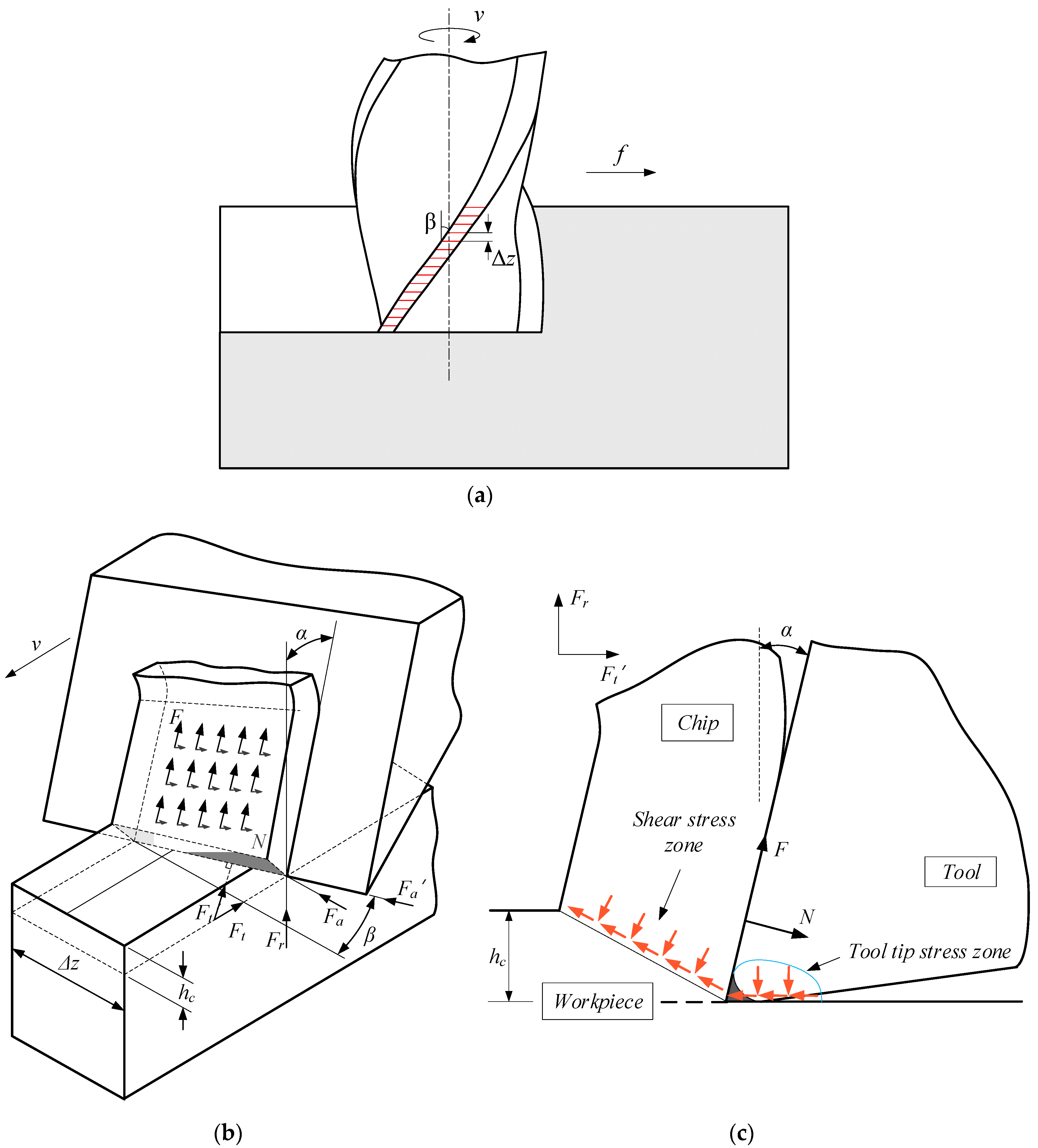
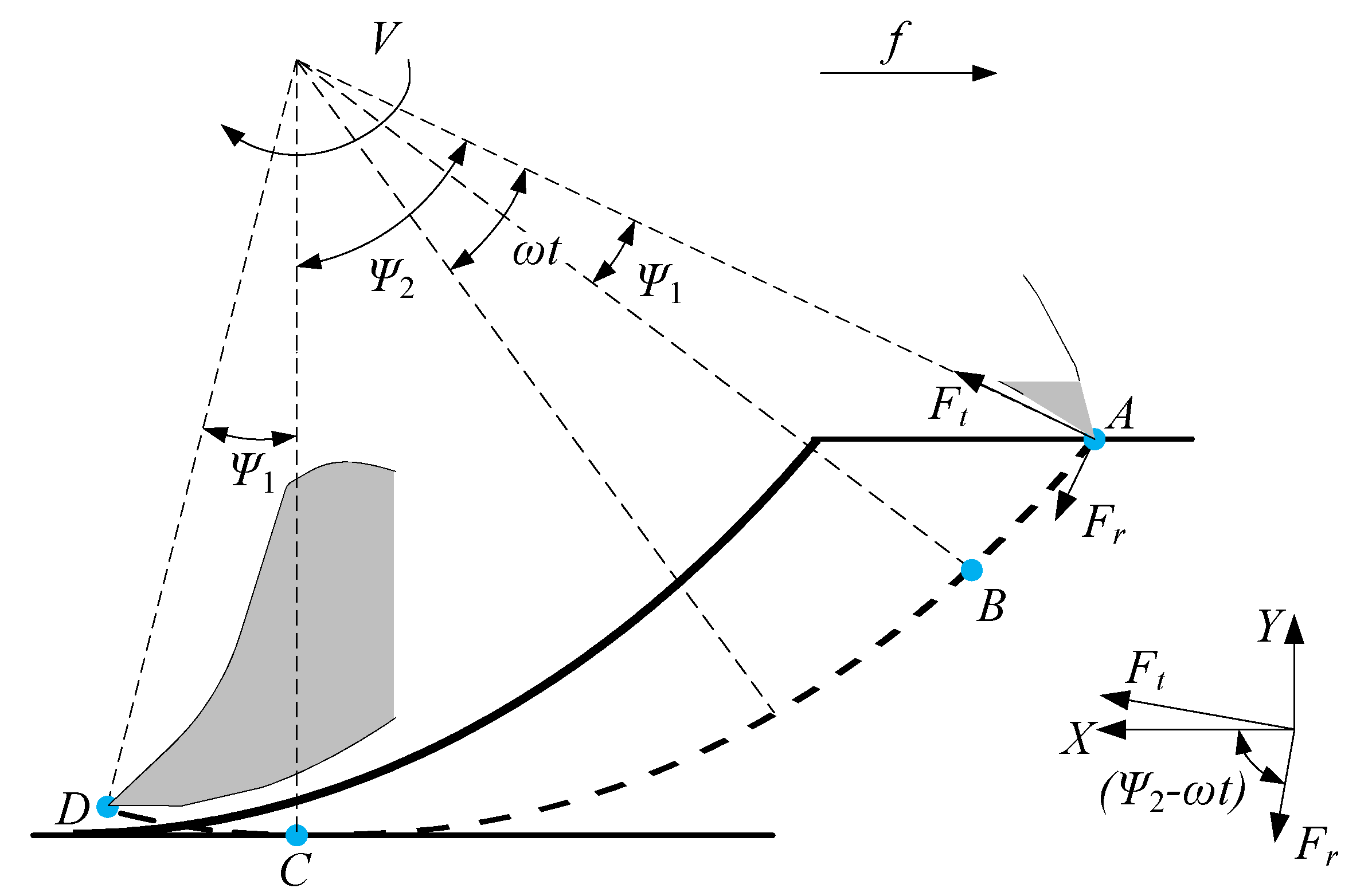
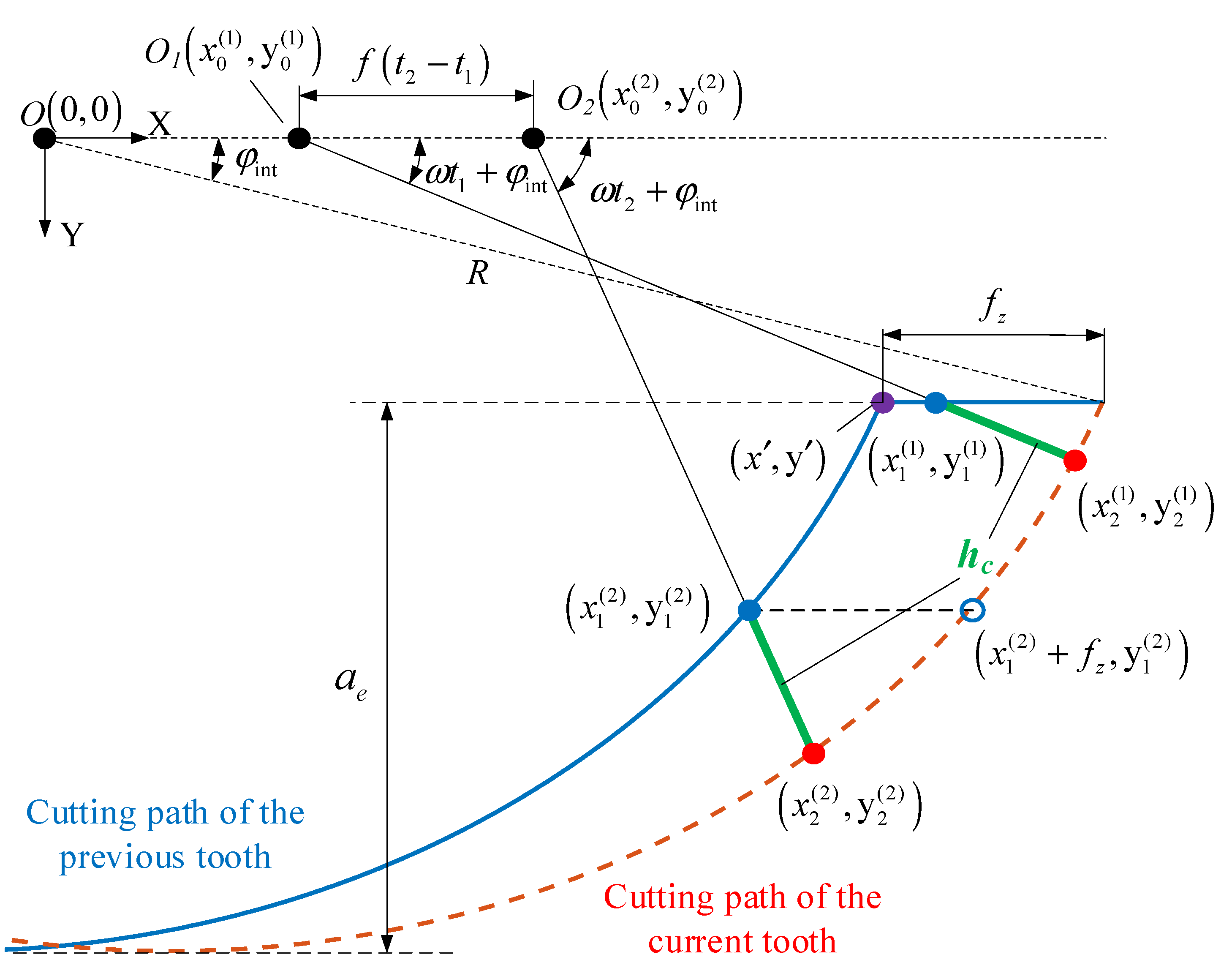
- Considering the thermal-mechanical coupling, a milling force model is established. Based on the thermo-mechanical coupling algorithm, the relative motion relationship between the tool and the workpiece during milling is analyzed, and a milling force model considering the thermal-mechanical coupling effect is established.
- (2)
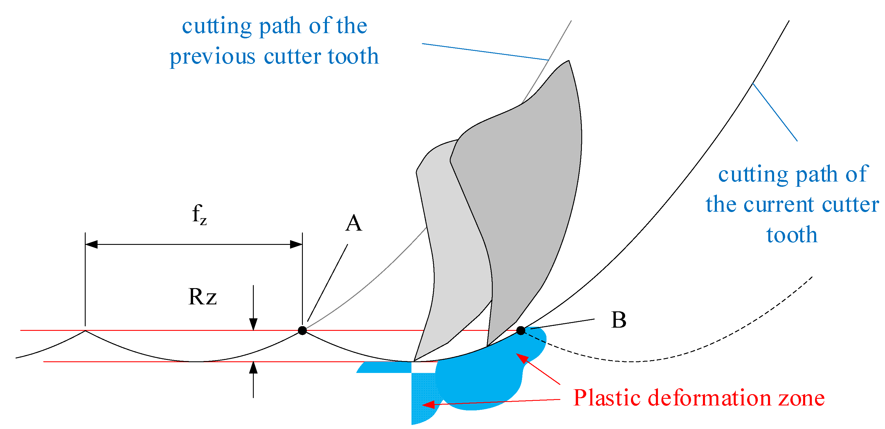
- Based on the milling force model, the residual stress prediction model is established. Considering the surface waviness of the workpiece after milling, an approximate assumption is proposed to planarize the machined surface to adapt to the residual stress analysis algorithm.
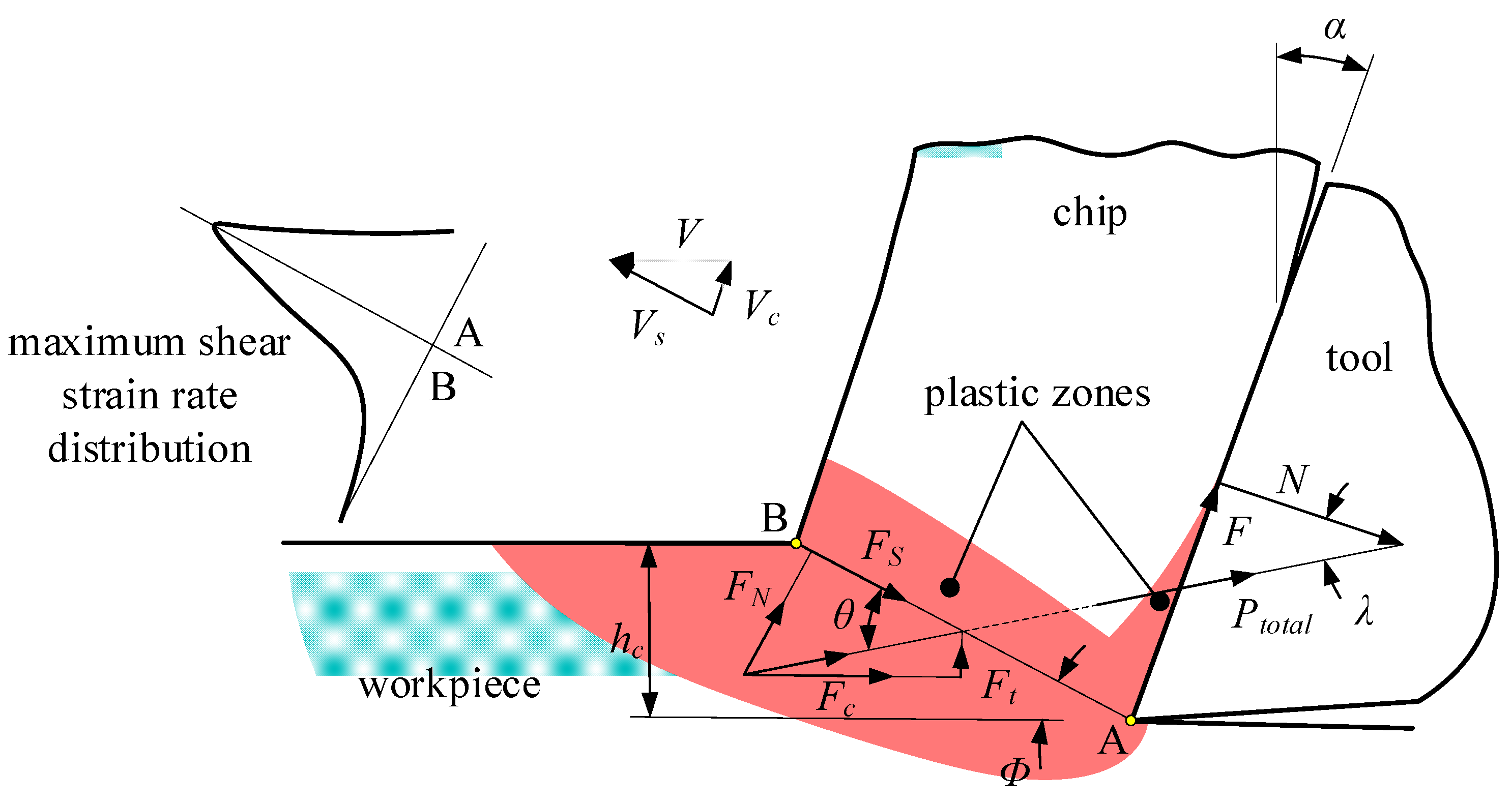
2. Research on Iterative Algorithm of Thermal-Mechanical Coupling in Orthogonal Cutting
- (1)
- There is no tool wear and cutting vibration, and no built-up edge is generated.
- (2)
- Plastic deformation in the cutting layer only occurs in a plane perpendicular to the cutting edge.
- (3)
- The primary and secondary deformation zones are assumed to be narrow area.
- (4)
- The temperature and strain on the shear plane are uniformly distributed.
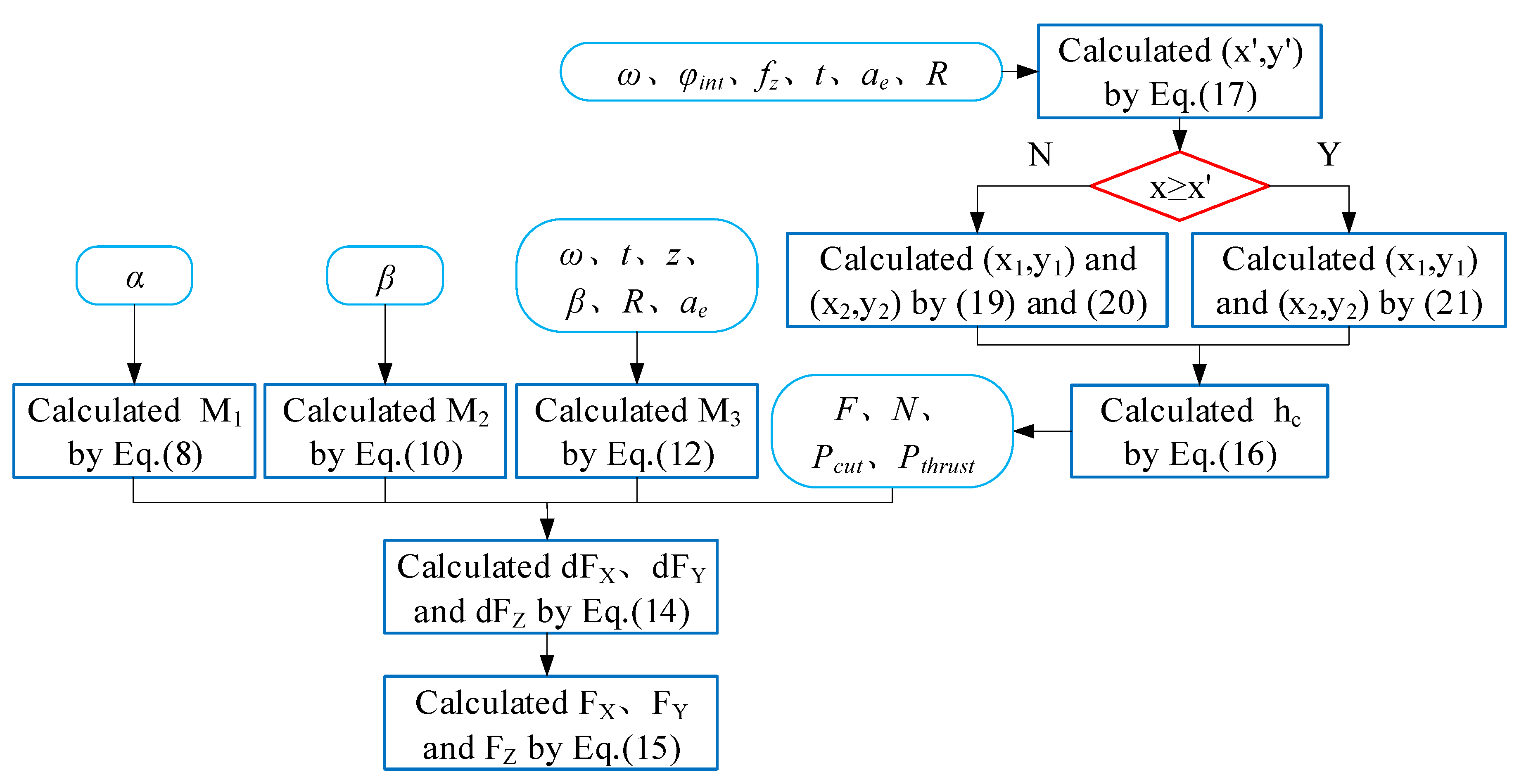
3. Milling Force Prediction Based on Analytical Method
4. Prediction of Residual Stress Considering Thermal-Mechanical Coupling Effect
4.1. Mechanical Stress Source and its Stress Distribution Model
4.2. Thermal Stress Source and its Stress Distribution Model
4.3. Hybrid Algorithm for Stress Loading Process
4.4. Stress Release Process
5. Experimental Validation of Milling Force Model and Residual Stress Model
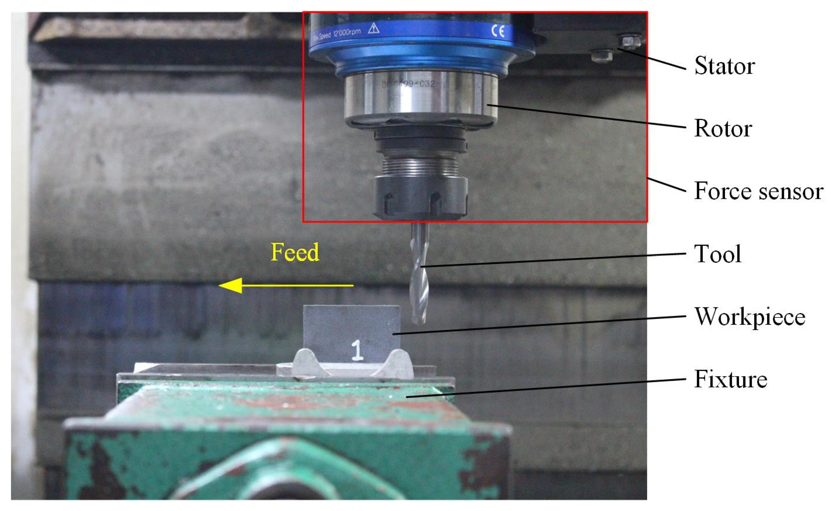
5.1. Experimental Machine Tool, Tool and Workpiece Material
5.2. Experimental Validation of Milling Force Model
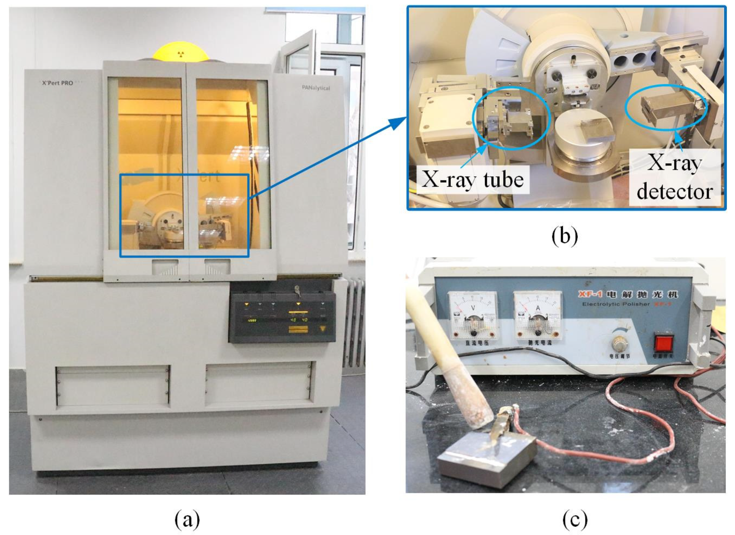
5.3. Measurement Device and Measurement Scheme for Residual Stress
5.4. Experimental Validation of Residual Stress Model
6. Conclusions
- (1)
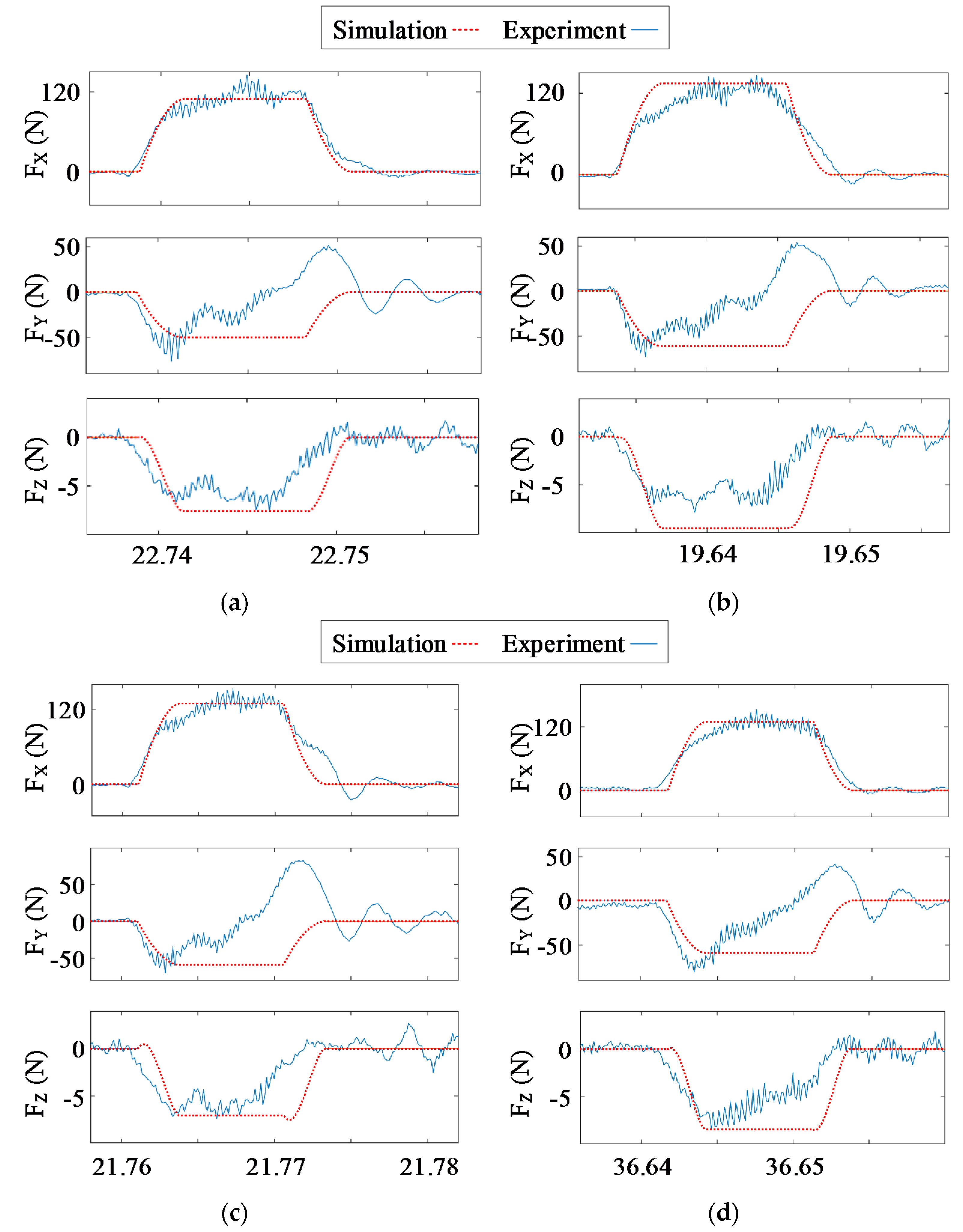
- The contact relationship between the tool and the workpiece during the milling is analyzed in detail. Compared with the milling forces FX and FZ, it can be found that there is still a wave value of convergence in the milling force FY after the tool cuts out from the workpiece, which proves that there is cutting vibration in the direction perpendicular to the workpiece. It is also found that the increase of radial cutting depth and feed rate will significantly increase the tool vibration. In the direction perpendicular to the workpiece surface, the milling force in the stable cutting stage fluctuates due to the influence of the cutter-drawing, but the milling forces FX and FZ can still be predicted well.
- (2)
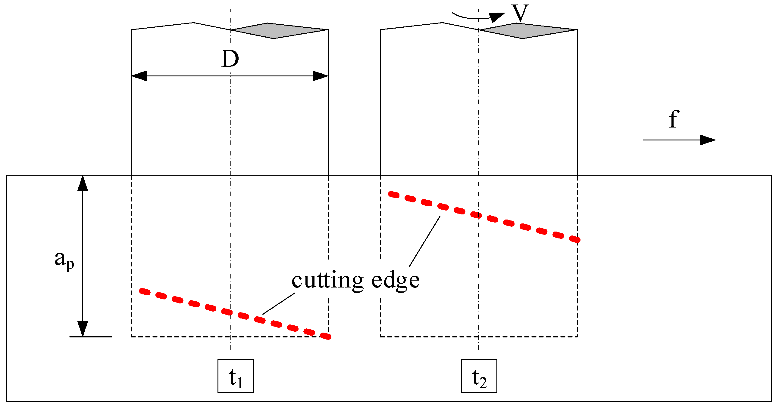
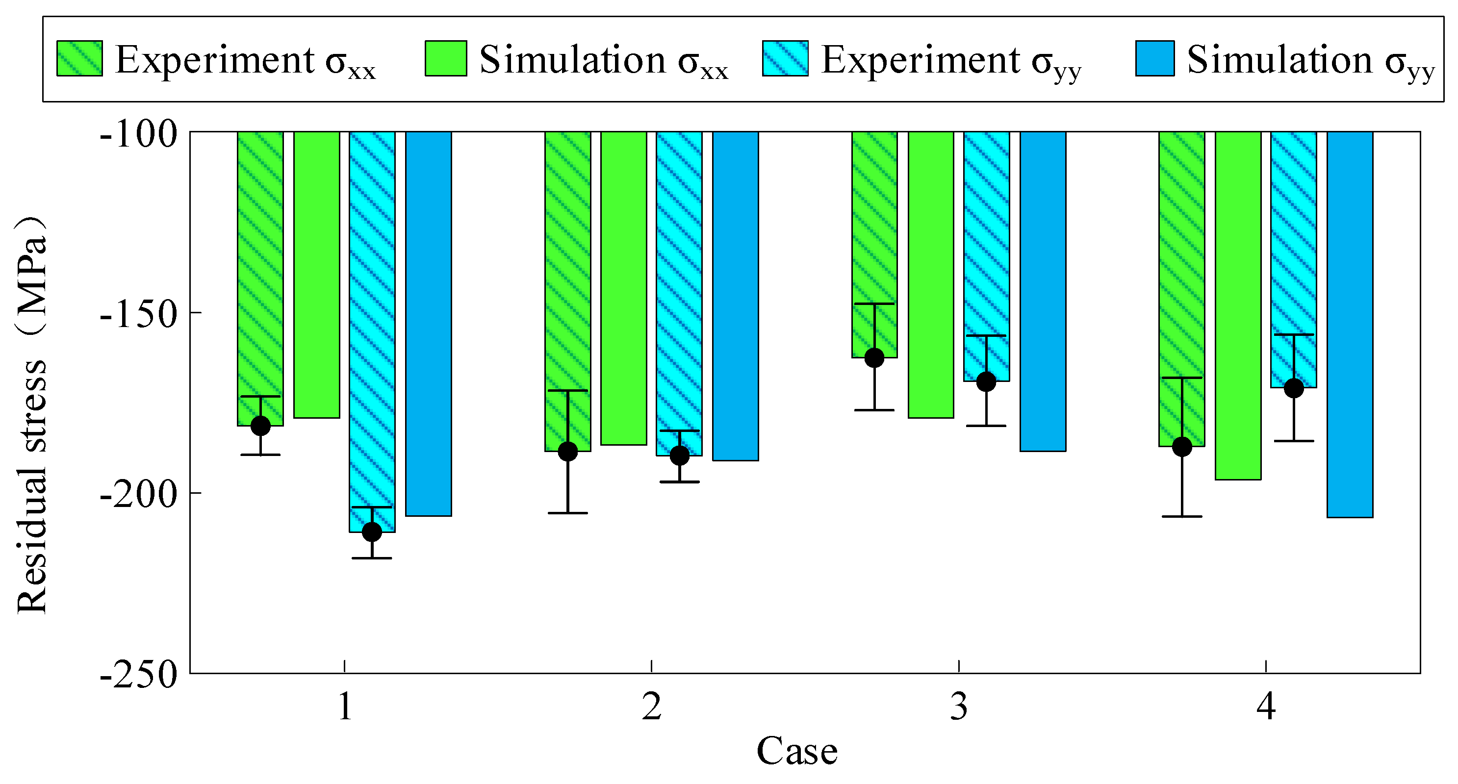
- In order to use the thermal coupling iterative algorithm and realize the rapid prediction of the peak value of the residual stress, the geometry of the workpiece surface is simplified. The residual stress model accurately predicted the peak value of the residual stress in the subsurface of the workpiece. With the increase of the radial cutting depth and feed rate, the cutting vibration will be intensified, the stress state in the surface of the workpiece will change, and the prediction error of the residual stress will increase.
- (3)
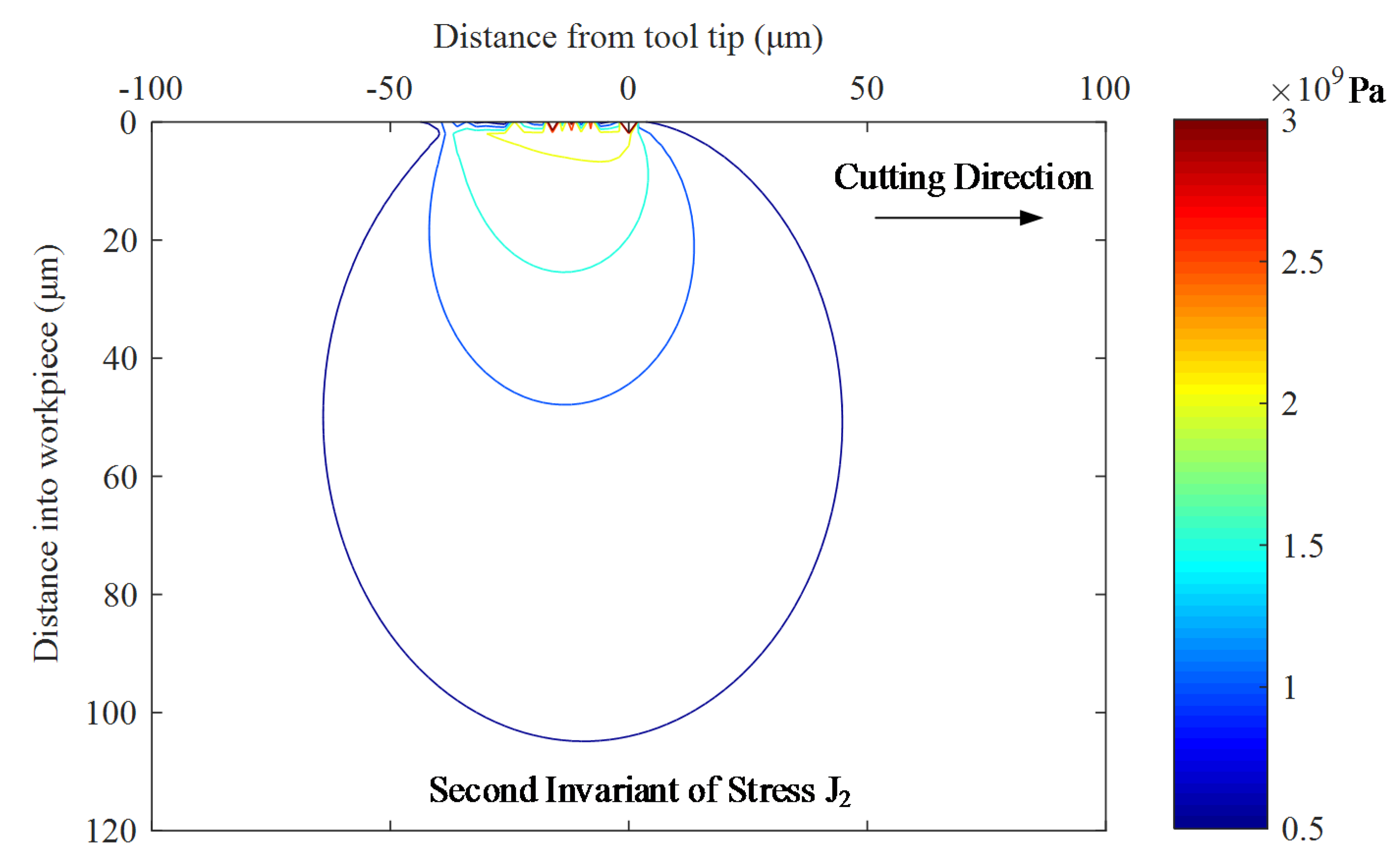
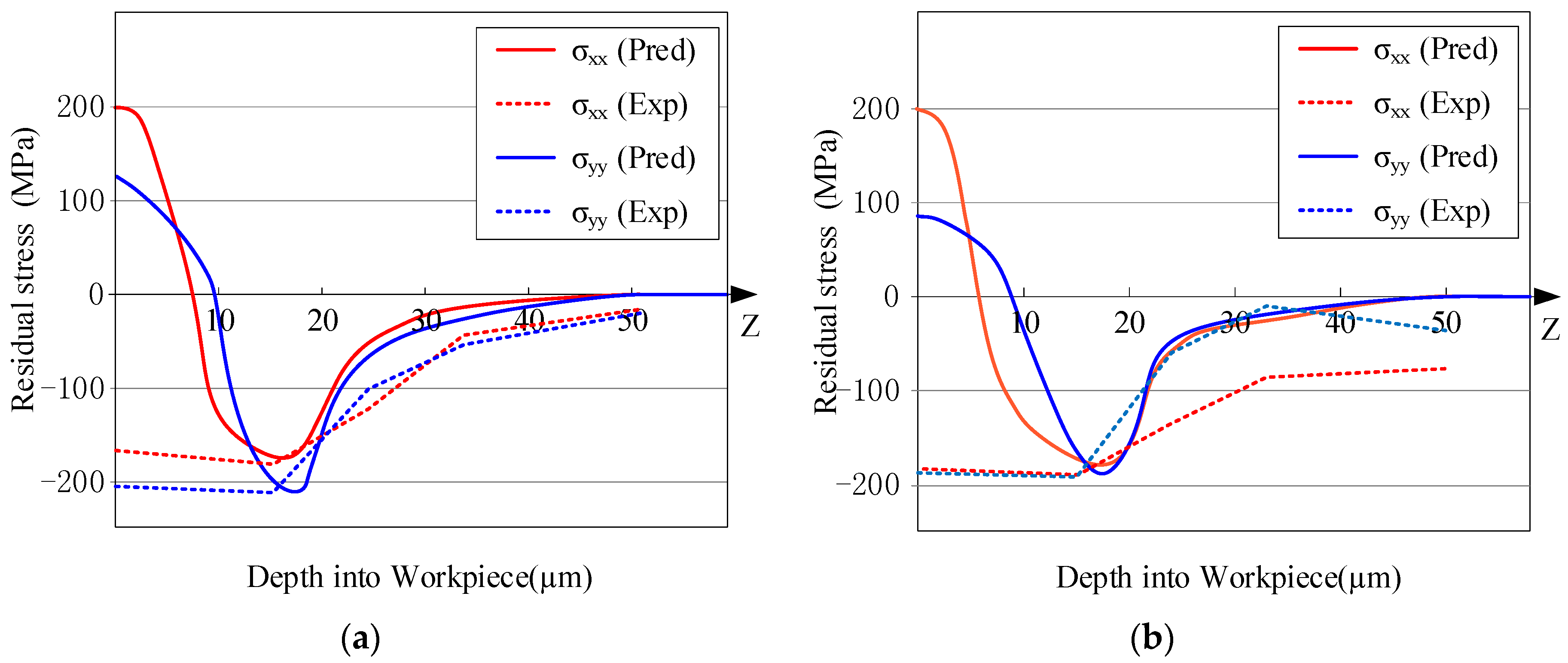
- According to the prediction results of residual stress, it can be seen that the influence depth of residual stress is about 50 μm and the depth of the peak value of subsurface residual stress is between 15 μm and 20 μm. The variation of residual stress σx and σy with depth is basically the same. The stress in the machined surface is tensile stress, and the peak value of subsurface stress is compressive stress, which may be due to the influence of cutting heat, resulting in a large tensile stress in the surface.
Author Contributions
Funding
Conflicts of Interest
Nomenclature
| ac | chip thermal diffusivity |
| B(x) | percentage of heat generated at the tool–chip interface entering the chip |
| Cp | Specific Heat Capacity |
| E | elastic modulus of the workpiece material |
| F | friction force at the rake face of the tool |
| f | feed rate |
| fz | feed per tooth |
| G | shear modulus of elasticity |
| h | plastic modulus |
| hc | cutting thickness |
| Kc | Thermal conductivity of the chip |
| Kt | Thermal conductivity of the tool |
| LAB | shear plane length |
| Lc | contact length between tool and chip |
| N | normal force at the rake face of the tool |
| nij | unit normal vector pointing outward the yield surface |
| Pthrust | plowing force normal to the newly generated surface |
| Pcut | plowing force in the cutting direction |
| Ptotal | resultant cutting force |
| qshear | heating source intensity in the primary shear zone |
| qf | heating source intensity in the second deformation zone |
| qrub | heating source intensity in the tertiary deformation zone |
| R | tool radius |
| sij | deviatoric stress |
| T0 | initial temperature |
| Tmelt | melting point |
| t | cutting time |
| Vc | chip velocity |
| v | Poisson’s ratio of the workpiece material |
| w | rotational speed of tool |
| wt | width of the cutting edge participating in cutting |
| z | axial height of the tool |
| α | rake angle of the tool |
| αT | thermal diffusion coefficient of the workpiece material |
| β | tool helix angle |
| λ | friction angle of the rake face. |
| Φ | shear angle of the primary shear zone |
| θ | angle between the force Ptotal and the shear plane AB |
| σAB | flow stress on the shear plane |
| γ | percentage of heat generated by the heat source qrub entering the tool |
| ρ | density |
| φint | cut-in angle |
References
- Su, J.C.; Young, K.A.; Ma, K.; Srivasta, S.; Morehouse, J.B.; Liang, S.Y. Modeling of residual stresses in milling. Int. J. Adv. Manuf. Technol. 2013, 65, 717–733. [Google Scholar] [CrossRef]
- Fergani, O.; Jiang, X.H.; Shao, Y.M.; Welo, T.; Yang, J.G.; Liang, S.Y. Prediction of residual stress regeneration in multi-pass milling. Int. J. Adv. Manuf. Technol. 2016, 83, 1153–1160. [Google Scholar] [CrossRef]
- Fergani, O.; Mkkadem, A.; Lazoglu, I.; Mansori, M.; Liang, S.Y. Analytical modelling of residual stress and the induced deflection of a milled thin plate. Int. J. Adv. Manuf. Technol. 2014, 75, 455–463. [Google Scholar] [CrossRef]
- Wang, S.Q.; Li, J.G.; He, C.L.; Xie, Z.Y. A 3D analytical model for residual stress in flank milling process. Int. J. Adv. Manuf. Technol. 2019, 104, 3545–3565. [Google Scholar] [CrossRef]
- Wan, M.; Ye, X.Y.; Yang, Y.; Zhang, W.H. Theoretical prediction of machining-induced residual stresses in three-dimensional oblique milling processes. Int. J. Mech. Sci. 2017, 133, 426–437. [Google Scholar] [CrossRef]
- Huang, K.; Yang, W. Analytical modeling of residual stress formation in workpiece material due to cutting. Int. J. Mech. Sci. 2016, 114, 21–34. [Google Scholar] [CrossRef]
- Huang, X.D.; Zhang, X.M.; Leopold, J.; Ding, H. Analytical model for prediction of residual stress in dynamic orthogonal cutting process. J. Manuf. Sci. Eng. 2018, 140, 011002. [Google Scholar] [CrossRef]
- Ji, X.; Zhang, X.P.; Liang, S.Y. A New Approach to Predict Machining Force and Temperature with Minimum Quantity Lubrication. In Proceedings of the ASME 2012 International Manufacturing Science and Engineering Conference (MSEC 2012), Notre Dame, IN, USA, 4–8 June 2012. [Google Scholar]
- Oxley, P.L.B.; Hastings, W.F. Predicting the strain rate in the zone of intense shear in which the chip is formed in machining from the dynamic flow stress properties of the work material and the cutting conditions. Proc. R. Soc. Lond. Ser. A 1977, 356, 395–410. [Google Scholar]
- Calamaz, M.; Coupard, D.; Girot, F. A new material model for 2D numerical simulation of serrated chip formation when machining titanium alloy Ti–6Al–4V. Int. J. Mach. Tool Manu. 2008, 48, 275–288. [Google Scholar] [CrossRef]
- Ducobu, F.; Rivière-Lorphèvre, E.; Filippi, E. Material constitutive model and chip separation criterion influence on the modeling of Ti6Al4V machining with experimental validation in strictly orthogonal cutting condition. Int. J. Mech. Sci. 2016, 107, 136–149. [Google Scholar] [CrossRef]
- Huang, Y.; Liang, S.Y. Cutting temperature modeling based on non-uniform heat intensity and partition ratio. Mach. Sci. Technol. 2005, 9, 301–323. [Google Scholar] [CrossRef]
- Saif, M.T.A.; Hui, C.Y.; Zehnder, A.T. Interface shear stresses induced by non-uniform heating of a film on a substrate. Thin Solid Films 1993, 224, 159–167. [Google Scholar] [CrossRef]
- Cotterell, M.; Byrne, G. Dynamics of chip formation during orthogonal cutting of titanium alloy Ti6Al4V. CIRP Ann. 2008, 57, 93–96. [Google Scholar] [CrossRef]
- Yue, C.X.; Gao, H.N.; Liu, X.L.; Liang, S.Y.; Wang, L.H. A review of chatter vibration research in milling. Chine. J. Aeronaut. 2019, 32, 215–242. [Google Scholar] [CrossRef]


| A (MPa) | B (MPa) | n | C | m | a | b | c | d | Tm (°C) | |
|---|---|---|---|---|---|---|---|---|---|---|
| 968 | 380 | 0.421 | 0.0197 | 0.577 | 0.1 | 1.6 | 0.4 | 6 | 1 | 1650 |
| Case | Spindle Speed (r/min) | Cutting Width (mm) | Cutting Depth (mm) | Feed Rate (mm/min) |
|---|---|---|---|---|
| 1 | 750 | 0.1 | 8 | 100 |
| 2 | 600 | 0.1 | 8 | 100 |
| 3 | 750 | 0.12 | 8 | 100 |
| 4 | 750 | 0.1 | 8 | 120 |
| Material Parameter | Ti6Al4V | WC |
|---|---|---|
| ρ (kg/m3) | 4430 | 15630 |
| K (W/m·°C) | 7.039e0.0011T | 55 |
| Cp (J/kg °C) | 505.64e0.0007T | 0.32T + 1.32 × 10⁻⁴ |
| Tmelt (°C) | 1650 | - |
| Case | in X Direction (N) | in Y Direction (N) | in Z Direction (N) |
|---|---|---|---|
| 1 | 10.61 | 37.64 | 2.53 |
| 2 | 22.06 | 51.49 | 4.57 |
| 3 | 15.33 | 52.75 | 2.60 |
| 4 | 13.39 | 37.25 | 3.06 |
| Plane (hkl) | Radiation | Bragg’s Angle 2θ | 1/2 S2 (MPa−1) | S1 (MPa−1) | Voltage (kV) | Current (mA) |
|---|---|---|---|---|---|---|
| (213) | Cu-Kα | 141.3° | 12.18 × 10⁻⁶ | −3.09 × 10⁻⁶ | 40 | 40 |
© 2020 by the authors. Licensee MDPI, Basel, Switzerland. This article is an open access article distributed under the terms and conditions of the Creative Commons Attribution (CC BY) license (http://creativecommons.org/licenses/by/4.0/).
Share and Cite
Yue, C.; Hao, X.; Ji, X.; Liu, X.; Liang, S.Y.; Wang, L.; Yan, F. Analytical Prediction of Residual Stress in the Machined Surface during Milling. Metals 2020, 10, 498. https://doi.org/10.3390/met10040498
Yue C, Hao X, Ji X, Liu X, Liang SY, Wang L, Yan F. Analytical Prediction of Residual Stress in the Machined Surface during Milling. Metals. 2020; 10(4):498. https://doi.org/10.3390/met10040498
Chicago/Turabian StyleYue, Caixu, Xiaole Hao, Xia Ji, Xianli Liu, Steven Y. Liang, Lihui Wang, and Fugang Yan. 2020. "Analytical Prediction of Residual Stress in the Machined Surface during Milling" Metals 10, no. 4: 498. https://doi.org/10.3390/met10040498
APA StyleYue, C., Hao, X., Ji, X., Liu, X., Liang, S. Y., Wang, L., & Yan, F. (2020). Analytical Prediction of Residual Stress in the Machined Surface during Milling. Metals, 10(4), 498. https://doi.org/10.3390/met10040498