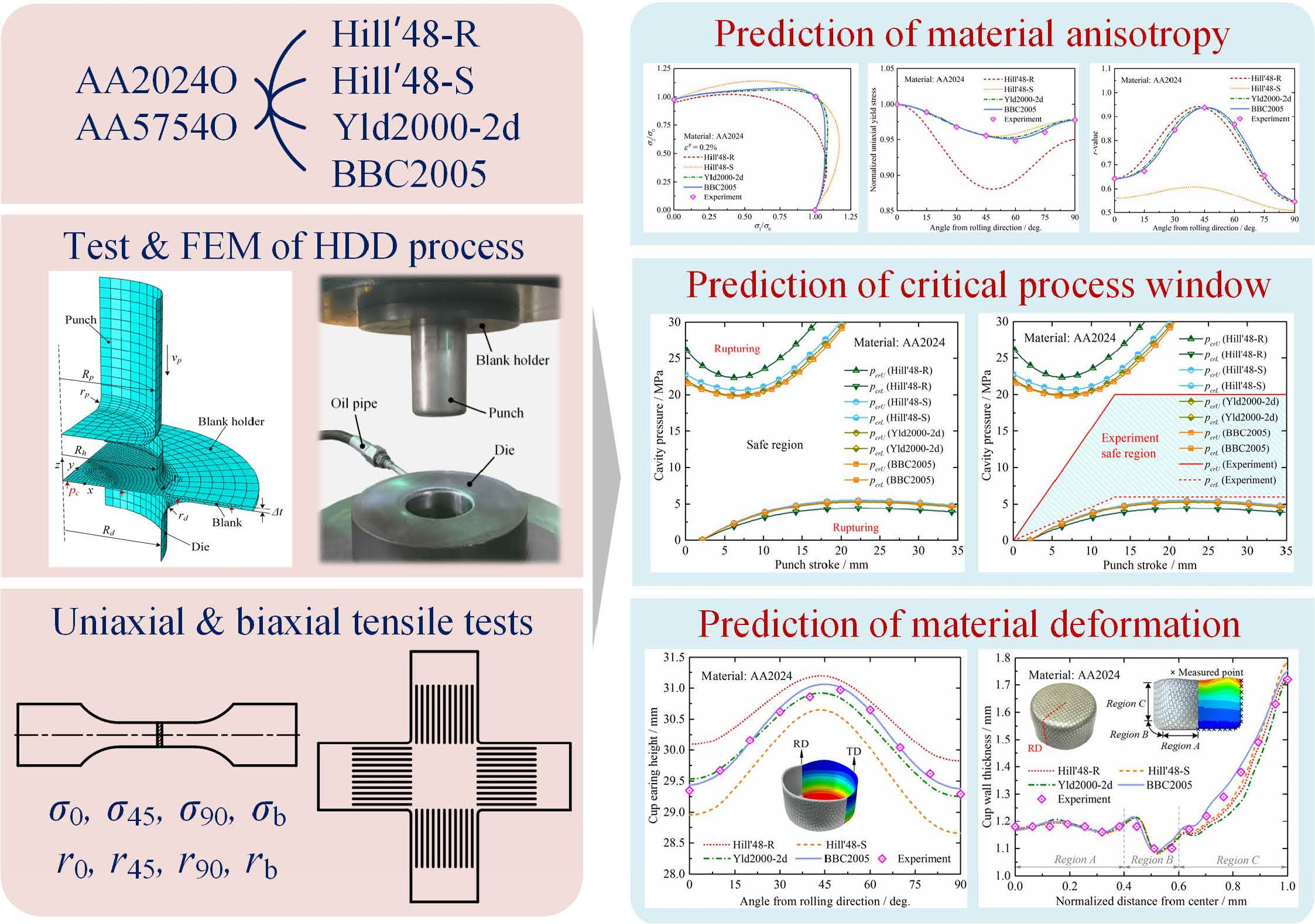
Effect of Anisotropic Yield Functions on Prediction of Critical Process Window and Deformation Behavior for Hydrodynamic Deep Drawing of Aluminum Alloys

Abstract

Owing to the reduction of rupture instability and the avoidance of wrinkle defect, the hydrodynamic deep drawing (HDD) process is gradually becoming attractive for fabricating lightweight and complicated products. Meanwhile, since metallic materials present anisotropic deformation behavior, it is necessary to select an appropriate constitutive model for the prediction of plastic deformation behavior of applied material with high precision. In the present research, several anisotropic yield criteria, namely, Hill’48, Yld2000-2d, and BBC2005, were implemented to investigate the effects of yield functions on the prediction accuracy of the critical process window and deformation behavior for the HDD process of 2024 and 5754 aluminum alloys. Material constants in the yield criteria were determined by applying uniaxial and equi-biaxial tension tests and optimizing an error-function using the Levenberg–Marquardt algorithm. Furthermore, the process window diagram was computed utilizing the stress analytical model combined material properties with workpiece geometrical features. Numerical simulation results of predicted material anisotropic parameters, process window, and HDD deformation for aluminum alloys were compared with the experimental data. Through the comparison of diverse yield criteria based on materials’ anisotropic coefficients, critical process window prediction, earing profile, and thickness distribution, it was revealed that the Yld2000-2d and the BBC2005 yield criteria can offer more precise models of material behavior in planar anisotropy properties for the HDD process of 2024 and 5754 aluminum alloys.

1. Introduction

Aluminum alloy is continuously being applied in the aerospace and automotive industry sectors because of their lightweight characteristic and excellent combination of strength and corrosion resistance. Complex aluminum alloy sheet metal parts with complicated shapes, large curvature variations, and deep cavities are constantly applied in the design of advanced aerospace structural parts. The deep drawing process is one of the significant manufacturing processes capable of fabricating thin-walled components which can not only reduce the cost but also enhance the performance of the products [1]. However, the formability of aluminum alloy is inadequate for the low ductility at room temperature and the high degree of springback. As a result, many aluminum alloy sheet metal parts cannot be fabricated using a one-step deep drawing process due to the complex structure and poor formability. For these reasons, a multi-step deep drawing process or partial forming with a welding method are applied to manufacture the complicated sheet metal parts, which results in defects such as excessive process redundancy, low forming accuracy, and poor forming quality. The utilization of flexible media in the deep drawing process has received increasing attention due to the multitude of its advantages such as improving sheet forming performance, forming efficiency, and convenient in mold changing. Hence, to surmount the difficulty in forming thin-walled aluminum alloy components, a better choice would be the hydrodynamic deep drawing (HDD) process [2,3].

The hydrodynamic deep drawing is a process that uses liquid as force transmission medium instead of conventional rigid die and makes the blank fit the punch under the pressure of liquid. A schematic of the HDD process is shown in Figure 1. During the forming period of the HDD process, the workpiece is pressed into the chamber through the punch. Meanwhile, a cushion of pressurized viscous fluid from the chamber is generated to support the noncontact region of the workpiece. Due to the fact of such external support, the provided through-thickness compressive stress contributes to delay the onset of tensile instability as well as to reduce the occurrence of wrinkles. Moreover, the workpiece bulges backward under the effect of pre-bulging pressure before the punch contacts the blank, which is a valid approach to avoiding the origination of the wrinkle on the unsupported region [4] as shown in Figure 2. The HDD process takes possession of many virtues in comparison with the conventional deep drawing (CDD) process including high dimensional accuracy, desirable surface quality, improved cold formability, less springback, and shortened manufacturing cycle [5,6]. Above all, the HDD process has superior performance on the avoidance of wrinkle phenomenon due to the controllable fluid pressure. Obviously, the cavity pressure of the chamber liquid is one of the most crucial parameters in the HDD process. As a result, determining the critical pressure and process window plays an important role in forming thin-walled workpieces without ruptures and wrinkle defects. In recent years, several researchers have devoted their investigations to the prediction of the critical pressure in the HDD process. Meng et al. [7] performed a series of finite element analyses for the HDD process of aluminum alloy rectangular boxes with wide flange. Meanwhile, the effects of cavity pressure on forming quality and precision were explored according to theoretical analysis and experiments, and the process window of cavity pressure was established through stress analysis of the corner and straight regions. Bagherzadeh et al. [8] developed analytical models to investigate stress distribution and instability conditions in hydro-mechanical deep drawing (HMDD) of cylindrical bimetallic cups. It was demonstrated that the fluid pressure window for successful part forming could be rapidly predicted with reasonable accuracy by the analytic model compared to lengthy and costly finite element analysis or experimental trial and error. Wang et al. [9] computed the process window for the HDD process of a composite conical part with double concave features. The optimal pressure loading loci were promoted based on the feature of workpiece.

Numerical simulation significantly contributes to reducing the overall production costs and inaccuracy in sheet metal forming industries by shortening both the time required in the R&D stage and the time needed for a corresponding production implementation [10,11]. Furthermore, the increasing application of numerical simulation in the field of sheet metal forming is beneficial to solve problems in the manufacturing of qualified formed parts [12,13]. Hence, the finite element method (FEM) has become an indispensable analysis tool in the manufacturing processes design. Liu et al. [14] proposed an analytical approach to obtain a proper prediction of liquid pressure for the hydroforming of a curved surface shell by the combination of numerical simulation and theoretical models. Moreover, the effects of different parameters for the proper liquid pressure were discussed using multiple linear regression analysis. Lang et al. [15] optimized the forming parameters in FEM of sheet hydroforming based on the identification of parameters for constitutive models by inverse modeling. Based on the optimized parameters, the sheet hydroforming process can be analyzed more accurately to improve the robust design. Gorji et al. [16] investigated the forming of conical–cylindrical cups in the HDD process using numerical simulation and experiments. It was also illustrated that for the pressure path with a specified maximum amount, the workpiece was formed adequately with minimum sheet thickness reduction.

The consistency of the decisions built on the FEM basis is highly dependent on the attained degree of the physical parameters and numerical accuracy of the simulation [17,18,19,20,21,22]. Many researchers involved in this domain focused their efforts on improving both the quality of the theoretical models implemented in the simulation programs and the efficiency of their applied computational strategies [23,24]. In this regard, the constitutive model providing an accurate description of the plastic anisotropy of HDD process has been the subject of numerous studies. Hashemi et al. [25] proposed a process window diagram to predict the minimum and maximum critical pressure in HDD of conical cups using the Hill’48 yield criterion numerically. Azodi et al. [26] developed analytical models based on the Barlat’89 and Hill’s non-quadratic yield criteria in the HMDD process to predict the maximum permissible fluid pressure with assuming plane strain tensile failure. Jalil et al. [3] developed theoretical models using the Barlat’89 yield criterion to analyze the critical bursting pressure in HDD of single- and double-layer sheets. According to the abovementioned research, it is generally believed that the Hill’48 and the Barlat’89 yield criteria can roughly describe the anisotropic plastic property of sheet metal, such as carbon steel and stainless steel, yet is unreasonable for the HDD process of aluminum alloys. Meanwhile, limited study has been reported for the applicable implementation of advanced anisotropic yield criteria for aluminum alloys in sheet hydroforming applications.

In this paper, the applicability of diverse anisotropic yield criteria, Hill’48, Yld2000-2d, and BBC2005, in theoretical analysis and numerical simulation of the HDD process of 2024 and 5754 aluminum alloys was carried out. A comparison between the numerical and experimental results is presented to evaluate the effectiveness of the selected yield criterion as well as the effect of the yield criterion on the prediction accuracy of process window and deformation behavior for HDD process of aluminum alloys in terms of forming force variation, thickness distribution, and earing phenomenon.

2. Anisotropic Yield Functions

The yield criterion expresses a relationship among the stress components in the transition from the elastic to the plastic regime which is a part of the most crucial criteria used in numerical simulation [27,28]. Due to the multi-pass rolling and heat treatment in the production process, aluminum alloy sheet presents remarkable anisotropic characteristics. The anisotropy of aluminum alloy has certain effects on the fracture position, earing, and forming limit of the part fabricating by HDD process. Therefore, the premise of accurately describing the deformation of aluminum alloy in the HDD process is to fully consider the influence of sheet anisotropy.

It can be mentioned that the most frequently applied yield criteria for the simulation of sheet metal forming process, Hill’s quadratic functions, have been fitted to equally many test results. It is noticeable that a constitutive model making full use of the available eight material parameters obtained from uniaxial and biaxial tests would be deeply in demand. Hence, one four-parameter anisotropic yield criterion namely, Hill’48, two eight-parameter anisotropic yield criteria namely, Yld2000-2d and BBC2005, were employed in this research as well as the numerical approach to evaluate material anisotropy and predict deformation for HDD process of aluminum alloys.

2.1. Hill’48 Yield Function

In 1948, Hill [29] proposed a constitutive formula for the plastic yielding and deformation of anisotropic metals at a macroscopic level. The quadratic yield criterion is given by Equation (1):

$$2f\left(\sigma \right)=F{\left({\sigma }_{yy}-{\sigma }_{zz}\right)}^2+G{\left({\sigma }_{zz}-{\sigma }_{xx}\right)}^2+H{\left({\sigma }_{xx}-{\sigma }_{yy}\right)}^2+2\left({L\tau }_{yz}^2+{M\tau }_{zx}^2+{N\tau }_{xy}^2\right)=1$$

(1)

where f is the yield function. σ_xx, σ_yy, and σ_zz are the stresses in the rolling, transverse, and thickness directions, respectively. τ_xy, τ_yz, and τ_zx are the shear stresses in the xy, yz, and zx planes, respectively. F, G, H, L, M, and N are the constants that describe the anisotropy of the material. Under the assumption of plane stress condition (σ_xx = τ_yz = τ_zx = 0), the yield criterion can be simplified as follow in Equation (2):

$$2f\left(\sigma \right)=\left(G+H\right){\sigma }_{xx}^2+\left(F+H\right){\sigma }_{yy}^2-{2H\sigma }_{xx}{\sigma }_{yy}+{2N\tau }_{xy}^2=1$$

(2)

In this study, the identification of the anisotropy parameters for Hill’48 model was carried out by applying two different methods. The classical approach uses the r values from three uniaxial tension tests (0°, 45°, and 90° to the rolling direction), which is labeled Hill’48-R. The second approach resorts to implementing the yield stresses from three uniaxial tension tests (0°, 45°, and 90° to the rolling direction), which is labeled Hill’48-S.

2.2. Yld2000-2d Yield Function

To alleviate the drawback of previous yield criteria in the description of yielding behavior of aluminum alloys, Barlat et al. [30] proposed the Yld2000-2d yield function which has eight anisotropy coefficients including tension yield stresses (i.e., σ₀, σ₄₅, σ₉₀) and r values (i.e., r₀, r₄₅, r₉₀) along the rolling direction, 45°, and the transverse directions as well as the yield stress σ_b and r_b under the balanced biaxial tension condition.

The equation for the yield locus of Yld2000-2d is given by Equation (3):

$$\chi ={\chi }^{\prime }+{\chi }^{″}=2{\overline{\sigma }}^m$$

(3)

with

$${\chi }^{\prime }={|\mathrm{X}}_1^{\prime }-{{\mathrm{X}}_2^{\prime }|}^m,{\chi }^{″}={|2\mathrm{X}}_2^{\prime }+{{\mathrm{X}}_1^{\prime }|}^m+{|2\mathrm{X}}_1^{″}+{{\mathrm{X}}_2^{″}|}^m$$

(4)

where m is the Barlat exponent relevant to the crystal structure of the material. In this research, m was 8 because of the FCC structure of the aluminum alloy. φ was the sum of the two anisotropic equations, i.e., φ’ and φ”. X’_i and X”_j (i, j = 1, 2) are the principal values of the matrixes X’ and X” which is expressed by Equation (5):

$$\{\begin{array}{l}{\mathrm{X}}_i^{\prime }=\frac{1}{2}\left({\mathrm{X}}_{11}^{\prime }+{\mathrm{X}}_{22}^{\prime }\pm \sqrt{{\left({\mathrm{X}}_{11}^{\prime }-{\mathrm{X}}_{22}^{\prime }\right)}^2+4{\mathrm{X}}_{12}^{\prime 2}}\right)\\ {\mathrm{X}}_j^{″}=\frac{1}{2}\left({\mathrm{X}}_{11}^{″}+{\mathrm{X}}_{22}^{″}\pm \sqrt{{\left({\mathrm{X}}_{11}^{″}-{\mathrm{X}}_{22}^{″}\right)}^2+4{\mathrm{X}}_{12}^{″2}}\right)\end{array}$$

(5)

The elements of X’ and X” are achieved from the following linear transformation of the Cauchy stress in Equation (6):

$$\{\begin{array}{l}{\mathbf{X}}^{\prime }={\mathit{L}}^{\prime }\mathit{\sigma }\\ {\mathbf{X}}^{″}={\mathit{L}}^{″}\mathit{\sigma }\end{array}$$

(6)

Here, L’ and L” are defined as follows in Equations (7)-(8):

$$\left[\begin{array}{c}{L}_{11}^{\prime }\\ L_{12}^{\prime }\\ L_{21}^{\prime }\\ \begin{array}{c}{L}_{22}^{\prime }\\ L_{66}^{\prime }\end{array}\end{array}\right]=\left[\begin{array}{ccc}\begin{array}{c}\begin{array}{c}2/3\\ -1/3\end{array}\\ \&0\\ \begin{array}{c}0\\ 0\end{array}\end{array}& \begin{array}{c}\begin{array}{c}0\\ 0\end{array}\\ 1/3\\ \begin{array}{c}2/3\\ 0\end{array}\end{array}& \begin{array}{c}\begin{array}{c}0\\ 0\end{array}\\ 0\\ \begin{array}{c}0\\ 1\end{array}\end{array}\end{array}\right]\left[\begin{array}{c}{\beta }_1\\ {\beta }_2\\ {\beta }_3\end{array}\right]$$

(7)

$$\left[\begin{array}{c}\begin{array}{c}{L}_{11}^{″}\\ L_{12}^{″}\end{array}\\ L_{21}^{″}\\ \begin{array}{c}{L}_{22}^{″}\\ L_{66}^{″}\end{array}\end{array}\right]=\frac{1}{9}\left[\begin{array}{ccc}\begin{array}{cc}\begin{array}{c}\begin{array}{c}-2\\ 1\end{array}\\ 4\\ \begin{array}{c}-2\\ 0\end{array}\end{array}& \begin{array}{c}\begin{array}{c}2\\ -4\end{array}\\ -4\\ \begin{array}{c}8\\ 0\end{array}\end{array}\end{array}& \begin{array}{c}\begin{array}{c}8\\ -4\end{array}\\ -4\\ \begin{array}{c}2\\ 0\end{array}\end{array}& \begin{array}{cc}\begin{array}{c}\begin{array}{c}-2\\ 4\end{array}\\ 1\\ \begin{array}{c}-2\\ 0\end{array}\end{array}& \begin{array}{c}\begin{array}{c}0\\ 0\end{array}\\ 0\\ \begin{array}{c}0\\ 9\end{array}\end{array}\end{array}\end{array}\right]\left[\begin{array}{c}\begin{array}{c}{\beta }_3\\ {\beta }_4\end{array}\\ {\beta }_5\\ \begin{array}{c}{\beta }_6\\ {\beta }_8\end{array}\end{array}\right]$$

(8)

where ${\beta }_1~{\beta }_8$ are eight anisotropy coefficients. In the model, the coefficients $L_{ij}^{\prime }$ and L”_ij can be described by the set of coefficients ${\beta }_1~{\beta }_8$. All these coefficients are defined independently. The r values and the yield stresses from uniaxial tensile tests of the specimens taken along 0°, 90°, and 45° to the rolling direction were taken into account. Besides, the equi-biaxial yield stress and r value were required for determining the remaining coefficients of the yield model.

2.3. BBC2005 Yield Function

The BBC2005 yield function is a plane stress yield criterion developed to describe the deformation behavior of the orthotropic sheet metal [31]. The yield surface function of BBC2005 yield criterion is defined as Equation (9):

$$\mathsf{\Phi }\left({\sigma }_{ij},Y\right)=\sigma \left({\sigma }_{ij}\right)-Y=0$$

(9)

where ${\sigma }_{ij}$ is the plane stress tensor. Y > 0 is an arbitrary reference yield stress. $\overline{\sigma }$ is the BBC2005 equivalent stress, given by Equation (10):

$$\overline{\sigma }={\left\{a{\left(\Lambda +\Gamma \right)}^{2k}+a{\left(\Lambda -\Gamma \right)}^{2k}+b{\left(\Lambda +\Psi \right)}^{2k}+b{\left(\Lambda -\Psi \right)}^{2k}\right\}}^{\frac{1}{2\mathrm{k}}}$$

(10)

where a and b are undetermined coefficients. The value of the integer exponent k can be adopted according to the crystallographic structure of the sheet metal: k = 3 for BCC alloys and k = 4 for FCC alloys. Γ, Λ, and Ψ are functions counting the planar components of the stress tensor which are given by Equation (11):

$$\Gamma ={\kappa }_1{\sigma }_{11}+{\kappa }_2{\sigma }_{22},\Lambda =\sqrt{{\left({\kappa }_5{\sigma }_{11}-{\kappa }_6{\sigma }_{22}\right)}^2+{\sigma }_{12}{\sigma }_{21}},\Psi =\sqrt{{\left({\kappa }_3{\sigma }_{11}-{\kappa }_4{\sigma }_{22}\right)}^2+{\sigma }_{12}{\sigma }_{21}}$$

(11)

where ${\kappa }_1$, ${\kappa }_2$, ${\kappa }_3$, ${\kappa }_4$, ${\kappa }_5$, and ${\kappa }_6$ are yield criterion constants.

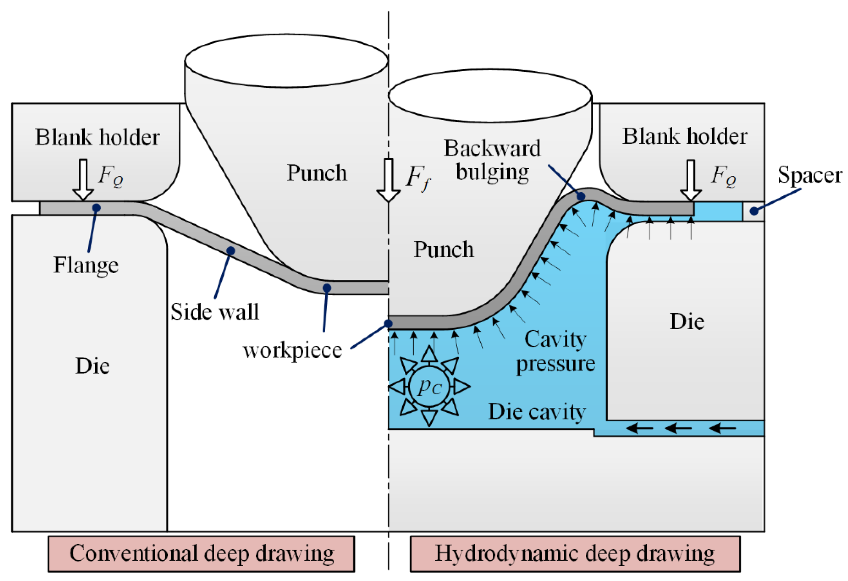
3. The Critical Process Window of HDD Process

In the HDD process, we proposed that the curve of chamber pressure with forming height is described as the cavity pressure loading locus. Only when a reasonable cavity pressure loading locus is designed within a certain range can the crack and wrinkle defects be avoided, and this area is defined as “critical process window” for the HDD process.

To analyze the critical process window of the sheet metal HDD process, several assumptions for calculating the critical cavity pressure are put forward as follows [32]:

(1) The volume of the workpiece is constant throughout the whole process;

(2) The radial and tangential directions are considered as principals;

(3) A nonlinear hardening plastic behavior of the material is assumed based on the power law. Hollomon’s equation expressed as Equation (12):

$$\overline{\sigma }=K{\overline{\epsilon }}^n$$

(12)

where $\overline{\epsilon }$, K, and n are the equivalent strain, strain hardening coefficient, and strain hardening exponent, respectively.

(4) The blank anisotropy can be depicted by the mean anisotropy coefficient ($\overline{r}$) as shown in Equation (13):

$$\overline{r}=\frac{r_0+{2r}_{45}+r_{90}}{4}$$

(13)

where $r_0$, $r_{45}$, and $r_{90}$ are Lankford coefficients describing the anisotropy.

The workpiece is divided into three regions according to the stress state including the corner flange area between the blank holder and the die (Region A), the curved region in contact with the pressurized fluid (Region B), and the area tightly compressed onto the surface of the punch due to the high pressure in chamber (Region C) as depicted in Figure 3.

In Figure 3, for an axisymmetric radial element in the flange area, the transformation of the thickness of the corner flange was assumed to be neglected. Considering the radial and tangential directions as principal directions in such an element, the equilibrium formula for the flange area of the radial direction is shown in Equation (14):

$$\frac{{t\mathrm{d}\sigma }_r}{\mathrm{d}r}+\frac{t}{r}\left({\sigma }_r-{\sigma }_{\theta }\right)+\mu p=0$$

(14)

where σ_r and σ_θ are the radial stress and circumferential stress. r is the radius of material element. t is the material thickness. μ is the friction coefficient between the workpiece and the blank holder. p is the fluid pressure under the flange along the vertical direction. R_b is the current radius of the outer flange. r_p is the profile radius of the punch shoulder. R_p is the radius of the punch. ρ is the radius of the part curvature around the die corner. h_p is the current cup height.

The stress state of Region B is similar to the flange area, while there is no friction force in this region due to the workpiece being completely separated from the die. The equilibrium formula in the normal direction of the workpiece in Figure 3 is depicted in Equation (15):

$$\frac{{t\mathrm{d}\sigma }_r}{\mathrm{d}r}+\frac{t}{r}\left({\sigma }_r-{\sigma }_{\theta }\right)=0$$

(15)

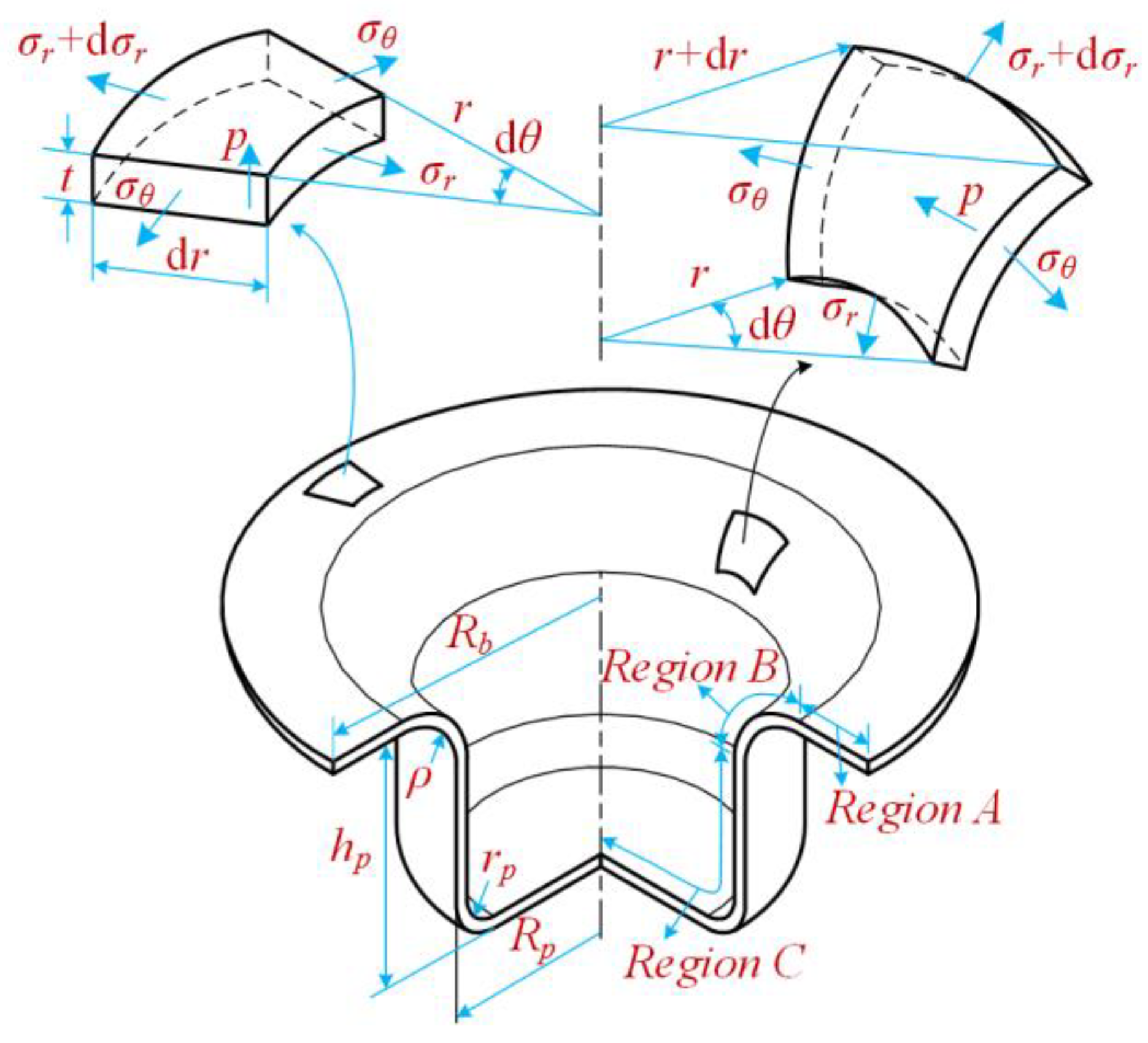
3.1. Analytical Modeling Applying the Hill’48 Yield Criterion

The associated flow rule was adopted which is expressed as follow in Equation (16):

$${\mathrm{d}\epsilon }_{ij}=\frac{\partial f}{\partial {\sigma }_{ij}}\mathrm{d}\lambda$$

(16)

where λ is the plastic multiplier and f is the plastic potential, defined as a scalar function described by the yield criterion. By applying the Hill’48 yield criterion, the flow rule is written in Equation (17):

$$\frac{{\mathrm{d}\epsilon }_1}{{\sigma }_1-\frac{\overline{r}}{1+\overline{r}}{\sigma }_2}=\frac{{\mathrm{d}\epsilon }_2}{{\sigma }_2-\frac{\overline{r}}{1+\overline{r}}{\sigma }_1}=\frac{-{\mathrm{d}\epsilon }_3}{\frac{{\sigma }_1+{\sigma }_2}{1+\overline{r}}}=\frac{\mathrm{d}\overline{\epsilon }}{\overline{\sigma }}$$

(17)

where dε₁, dε₂, and dε₂ are the plastic strain incremental components along the principal directions.

Considering the radial and tangential directions as principal directions, Equation (17) results in:

$${\sigma }_r-{\sigma }_{\theta }=\frac{\left(1+\overline{r}\right)\overline{\sigma }\left({\mathrm{d}\epsilon }_r-{\mathrm{d}\epsilon }_{\theta }\right)}{\left(1+2\overline{r}\right)\mathrm{d}\overline{\epsilon }}$$

(18)

Ignoring the thickness variations (${\mathrm{d}\epsilon }_r{=\mathrm{d}\epsilon }_{\theta }$), the effective strain can be obtained as Equation (19):

$$\overline{\epsilon }={\epsilon }_r\sqrt{\frac{2\left(1+\overline{r}\right)}{1+2\overline{r}}}$$

(19)

By substituting Equations (18) and (19) into Equation (14) and integrating, the radial stress of the workpiece in Region A is:

$${\sigma }_r^{\left(1\right)}=K{\left\{\frac{2\left(1+\overline{r}\right)}{1+2\overline{r}}\right\}}^{\frac{\left(n+1\right)}{2}}{{\displaystyle \int }}_r^{R_b}\frac{1}{r}{\left(\ln \frac{r_0^{\left(1\right)}}{r^{\left(1\right)}}\right)}^n\mathrm{d}r+p\left\{\frac{\mu }{t}\left(R_b-r\right)-1\right\}$$

(20)

where $r^{\left(1\right)}$ is the current radius in Region A, and $r_0^{\left(1\right)}$ is the initial radius of a supposed point in the flange region that moved to the current point with radius $r^{\left(1\right)}$.

Adopting the volume constancy condition, the relationship between $r^{\left(1\right)}$ and $r_0^{\left(1\right)}$ in Region A can be defined as the following in Equation (21) with the condition $R_p+t+\rho \le r\le R_b$.

$$\begin{gathered} {\left(r_0^{\left(1\right)}\right)}^2=r^2-{\left(R_p+t+\rho \right)}^2+{2R}_p\left(H_p-t-\rho -r_p\right) \\ +{\left(R_p-r_p\right)}^2+\pi \left(t+\rho \right)\left(R_p+t+\rho -\frac{2t+2\rho }{\pi }\right)+{\pi r}_p\left(R_p-r_p+\frac{{2r}_p}{\pi }\right) \end{gathered}$$

(21)

The current flange radius is determined as Equation (22):

$$\begin{gathered} R_b^2=R_0^2+{\left(R_p+t+\rho \right)}^2-{2R}_p\left(H_p-t-\rho -r_p\right)+{\left(R_p-r_p\right)}^2 \\ -\pi \left(t+\rho \right)\left(R_p+t+\rho -\frac{2t+2\rho }{\pi }\right)-{\pi r}_p\left(R_p-r_p+\frac{{2r}_p}{\pi }\right) \end{gathered}$$

(22)

With regard to the boundary condition, the radial stress of the workpiece based on the Hill’48 yield criterion in Region B is calculated by Equation (23):

$${\sigma }_r^{\left(2\right)}\left(r\right)=K{\left\{\frac{2\left(1+\overline{r}\right)}{1+2\overline{r}}\right\}}^{\frac{\left(n+1\right)}{2}}{{\displaystyle \int }}_r^{R_2+t+\rho }\frac{1}{r}{\left(\mathrm{In}\frac{r_0^{\left(2\right)}}{r^{\left(2\right)}}\right)}^n\mathrm{d}r+{\sigma }_r^{\left(1\right)}\left(r=R_p+t+\rho \right)$$

(23)

where $r^{\left(2\right)}$ is the current radius in Region B.

The relation between the current and initial radius of the material element in Region B is defined as following Equation (24) with the condition $R_b\le r\le R_p+t+\rho$.

$$\begin{gathered} {\left(r_0^{\left(2\right)}\right)}^2=2\left(t+\rho \right)\left\{\left(R_p+t+\rho \right)\phi -\left(t+\rho \right)\sin \phi \right\}+{\left(R_p-r_p\right)}^2 \\ +\pi \left(t+\rho \right)\left(R_p+t+\rho -\frac{2t+2\rho }{\pi }\right)+{2R}_p\left(H_p-t-\rho -r_p\right) \end{gathered}$$

(24)

where $\phi =\arccos \left(\frac{R_p-r}{t+\rho }+1\right)$ and $\rho =\sqrt{1+\frac{{2t\sigma }_r\left(R_p\right)}{{pR}_p}}-1$.

3.2. Analytical Modeling Applying the Yld2000-2d Yield Criterion

According to the plane strain assumption, the effective stress as a function with the ratio of tangential to radial stress ($\gamma ={\sigma }_2/{\sigma }_1$) can be written as Equation (25):

$$\overline{\sigma }={\sigma }_1^m\cdot l\left(\gamma \right)={\sigma }_1^m\cdot \frac{1}{2}\left({\left(v_1+v_2\gamma \right)}^m+{\left(v_3-v_4\gamma \right)}^m+{\left(v_5+v_6\gamma \right)}^m\right)$$

(25)

where

$$\begin{gathered} v_1=L_{11}^{\prime }+L_{21}^{\prime },v_2=L_{12}^{\prime }+L_{22}^{\prime },v_3=L_{11}^{″}+L_{21}^{″} \\ {v}_4=L_{12}^{″}+{2L}_{22}^{″},v_5={2L}_{11}^{″}+L_{21}^{″},v_6={2L}_{12}^{″}+L_{22}^{″} \end{gathered}$$

(26)

Substituting Equation (25) into the flow rule equation results in Equation (27):

$$\frac{{\mathrm{d}\epsilon }_1}{\frac{\partial \chi }{\partial {\sigma }_1}}=\frac{{\mathrm{d}\epsilon }_2}{\frac{\partial \chi }{\partial {\sigma }_2}}=\frac{-{\mathrm{d}\epsilon }_3}{\frac{\partial \chi }{\partial {\sigma }_1}+\frac{\partial \chi }{\partial {\sigma }_2}}=\frac{\mathrm{d}\overline{\epsilon }}{\overline{\sigma }}$$

(27)

where

$$\frac{\partial \phi }{\partial {\sigma }_1}={\sigma }_1^{m-1}m\left(\gamma \right),\frac{\partial \phi }{\partial {\sigma }_2}={\sigma }_1^{m-1}n\left(\gamma \right)$$

(28)

with

$$\begin{gathered} m\left(\gamma \right)=\frac{1}{2}m\left\{v_1{\left(v_1+v_2\gamma \right)}^{m-1}+v_3{\left(v_3-v_4\gamma \right)}^{m-1}+v_5{\left(v_5+v_6\gamma \right)}^{m-1}\right\} \\ n\left(\gamma \right)=\frac{1}{2}m\left\{v_1{\left(v_1+v_2\gamma \right)}^{m-1}-v_3{\left(v_3-v_4\gamma \right)}^{m-1}+v_5{\left(v_5+v_6\gamma \right)}^{m-1}\right\} \end{gathered}$$

(29)

Neglecting the thickness strain (${\mathrm{d}\epsilon }_1=-{\mathrm{d}\epsilon }_2$), the strain work is written as Equation (30):

$${\sigma }_r-{\sigma }_{\theta }=K{\overline{\epsilon }}^n\frac{\mathrm{d}\overline{\epsilon }}{{\mathrm{d}\epsilon }_r}$$

(30)

The effective strain can be obtained as Equation (31):

$$\mathrm{d}\overline{\epsilon }=\frac{\left(1-\gamma \right)}{l\left(\gamma \right)}{\mathrm{d}\epsilon }_r$$

(31)

By substituting Equations (30) and (31) into Equation (14) and integrating, the radial stress of the workpiece in Region A is:

$${\sigma }_r^{\left(1\right)}=K\frac{\left(1-\gamma \right)}{l\left(\gamma \right)}{{\displaystyle \int }}_r^{R_b}\frac{1}{r}\ln {\left(\frac{r_0^{\left(1\right)}}{r^{\left(1\right)}}\right)}^n\mathrm{d}r+p\left(\frac{\mu }{t}\left(R_b-r\right)-1\right)$$

(32)

Considering the plane stress assumption, γ can be obtained by solving $m\left(\gamma \right)/n\left(\gamma \right)=-1$.

Therefore, the radial stress of the workpiece element based on the Yld2000-2d yield criterion in Region B is:

$${\sigma }_r^{\left(2\right)}=K\frac{\left(1-\gamma \right)}{l\left(\gamma \right)}{{\displaystyle \int }}_r^{R_b+t+\rho }\frac{1}{r}\ln {\left(\frac{r_0^{\left(2\right)}}{r^{\left(2\right)}}\right)}^n\mathrm{d}r+{\sigma }_r^{\left(1\right)}\left(r=R_p+t+\rho \right)$$

(33)

3.3. Analytical Modeling Applying the BBC2005 Yield Criterion

The effective stress of the BBC2005 yield function can be written as Equation (34):

$$\overline{\sigma }={\sigma }_1^{2k}\cdot \left[a{\left(u_1+u_2\gamma \right)}^{2k}+a{\left(u_3+u_4\gamma \right)}^{2k}+b{\left(u_5+u_6\gamma \right)}^{2k}+b{\left(u_7+u_8\gamma \right)}^{2k}\right]$$

(34)

where

$$\begin{gathered} u_1={\kappa }_1+{\kappa }_5,u_2={\kappa }_2-{\kappa }_6,u_3={\kappa }_1-{\kappa }_5,u_4={\kappa }_2+{\kappa }_6 \\ {u}_5={\kappa }_5+{\kappa }_3,u_6={\kappa }_6+{\kappa }_4,u_7={\kappa }_5-{\kappa }_3,u_8={\kappa }_6-{\kappa }_4 \end{gathered}$$

(35)

Substituting Equation (9) into the flow rule equation results in Equation (36):

$$\frac{{\mathrm{d}\epsilon }_1}{\frac{\partial \Phi }{\partial {\sigma }_1}}=\frac{{\mathrm{d}\epsilon }_2}{\frac{\partial \Phi }{\partial {\sigma }_2}}=\frac{-{\mathrm{d}\epsilon }_3}{\frac{\partial \Phi }{\partial {\sigma }_1}+\frac{\partial \Phi }{\partial {\sigma }_2}}$$

(36)

where

$$\frac{\partial \Phi }{\partial {\sigma }_1}={\sigma }_1^{2k-1}j\left(\gamma \right),\frac{\partial \Phi }{\partial {\sigma }_2}={\sigma }_1^{2k-1}k\left(\gamma \right)$$

(37)

The functions j(γ) and k(γ) are defined as Equation (38):

$$\begin{gathered} j\left(\gamma \right)=2k\left\{\begin{array}{c}{au}_1{\left(u_1+u_2\gamma \right)}^{2k-1}+{au}_3{\left(u_3+u_4\gamma \right)}^{2k-1}\\ +{bu}_5{\left(u_5+u_6\gamma \right)}^{2k-1}+{bu}_7{\left(u_7+u_8\gamma \right)}^{2k-1}\end{array}\right\} \\ k\left(\gamma \right)=2k\left\{\begin{array}{c}{au}_2{\left(u_1+u_2\gamma \right)}^{2k-1}+{au}_4{\left(u_3+u_4\gamma \right)}^{2k-1}\\ -{bu}_6{\left(u_5+u_6\gamma \right)}^{2k-1}-{bu}_8{\left(u_7+u_8\gamma \right)}^{2k-1}\end{array}\right\} \end{gathered}$$

(38)

The strain work solution of the BBC2005 is similar to the Yld2000-2d one; it is obtained as:

$${\sigma }_r-{\sigma }_{\theta }=K{\overline{\epsilon }}^n\frac{\left(1-\gamma \right)}{h\left(\gamma \right)}$$

(39)

By substituting Equation (39) into Equation (14) and integrating, the radial stress of the workpiece in Region A is:

$${\sigma }_r^{\left(1\right)}=K\frac{\left(1-\gamma \right)}{h\left(\gamma \right)}{{\displaystyle \int }}_r^{R_b}\frac{1}{r}\ln {\left(\frac{r_0^{\left(1\right)}}{r^{\left(1\right)}}\right)}^n\mathrm{d}r+p\left\{\frac{\mu }{t}\left(R_b-r\right)-1\right\}$$

(40)

Therefore, the radial stress of the workpiece element based on the BBC2005 yield criterion in Region B is in Equation (41):

$${\sigma }_r^{\left(2\right)}=K\frac{\left(1-\gamma \right)}{h\left(\gamma \right)}{{\displaystyle \int }}_r^{R_b+t+\rho }\frac{1}{r}\ln {\left(\frac{r_0^{\left(2\right)}}{r^{\left(2\right)}}\right)}^n\mathrm{d}r+{\sigma }_r^{\left(1\right)}\left(r=R_p+t+\rho \right)$$

(41)

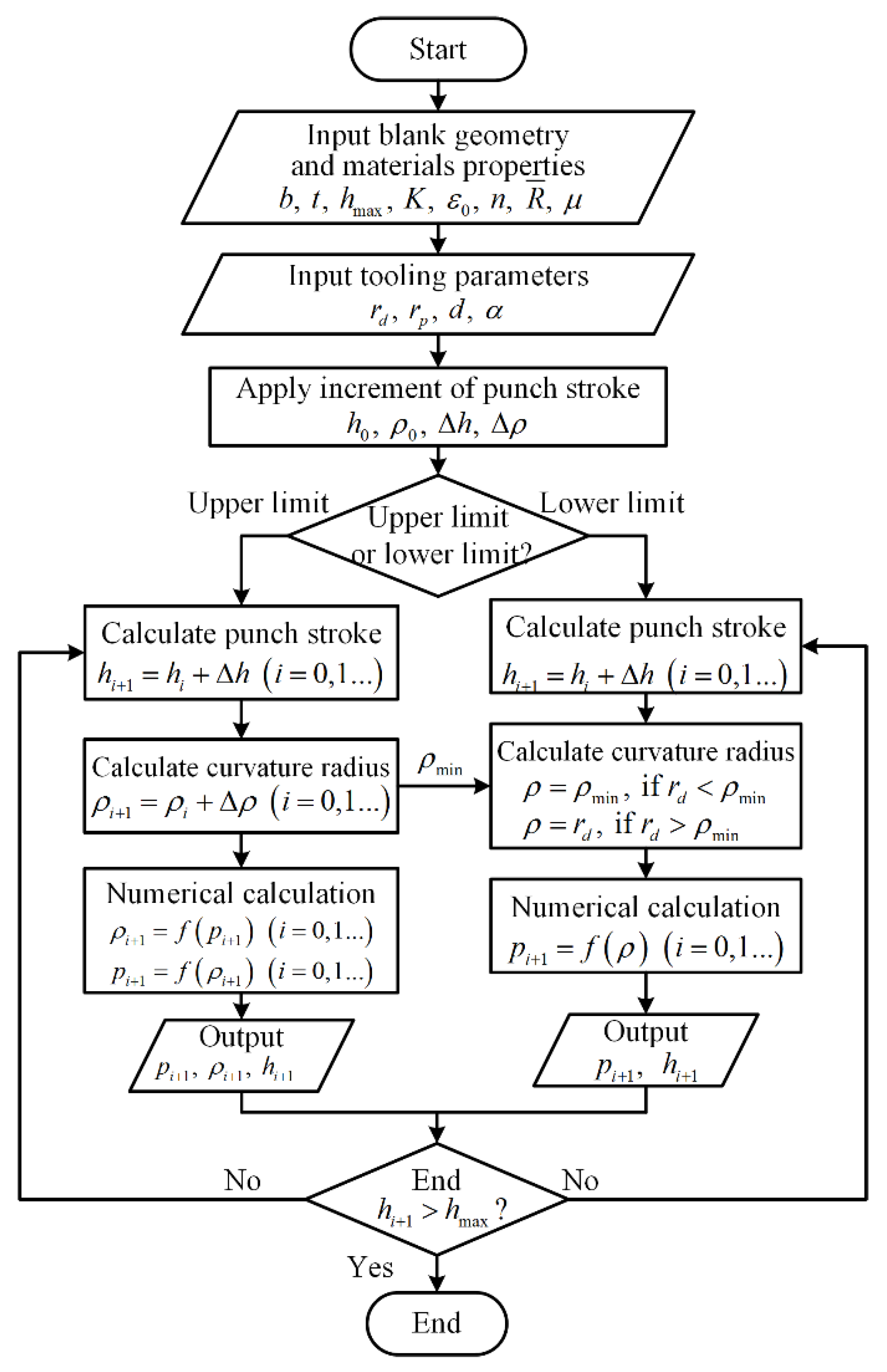
3.4. Critical Cavity Pressure

During the HDD process, the punch force (F_p) exerted on the workpiece and the equilibrium equation in the vertical direction of the workpiece are expressed as follows in Equations (42) and(43):

$$F_p=2\pi t\left(R_p+t\right){\sigma }_z^{\left(3\right)}+{2\pi \mu pR}_p\left(h_p-t-\rho \right)+{\pi R}_p^{2}p$$

(42)

$$\pi p\left\{{\left(R_p+t+\rho \right)}^2-{\left(R_p+t\right)}^2\right\}={2\pi R}_p{t\sigma }_r^{\left(2\right)}{(R}_p)$$

(43)

The maximum tensile stress of the unsupported area (Region B) should not exceed the tensile strength of used material is the principle to calculate the upper critical pressure of critical process window. Therefore, the necking condition occurs around the punch corner and the forming force curve experiences the maximum point (dF_p=0). When the cavity pressure is exceedingly higher, the fracture may appear around the die radius area. The specific procedure for calculating the upper critical pressure is referred to in a previous study [7].

The workpiece is separated from the die corner under the effect of cavity pressure to decrease the friction between the blank and the die. According to the critical geometric condition ($\rho =r_d$) and equilibrium equation, i.e., Equation (42), the lower critical cavity pressure can be presented as Equation (44):

$$p_l={\frac{{2tR}_p\cdot {\sigma }_r^{\left(2\right)}\left(R_p\right)}{\rho \left({2R}_p+2t+\rho \right)}|}_{\rho =r_d}$$

(44)

Calculation procedures for the critical process window is represented by the flow chart in Figure 4. All the calculation steps were executed utilizing Newton’s method in MATLAB R2018b numerical computing language. The initial values of h_p and ρ were set as 0. Furthermore, the values of Δh and Δρ were specified to be 0.05 and 0.1 mm, respectively.

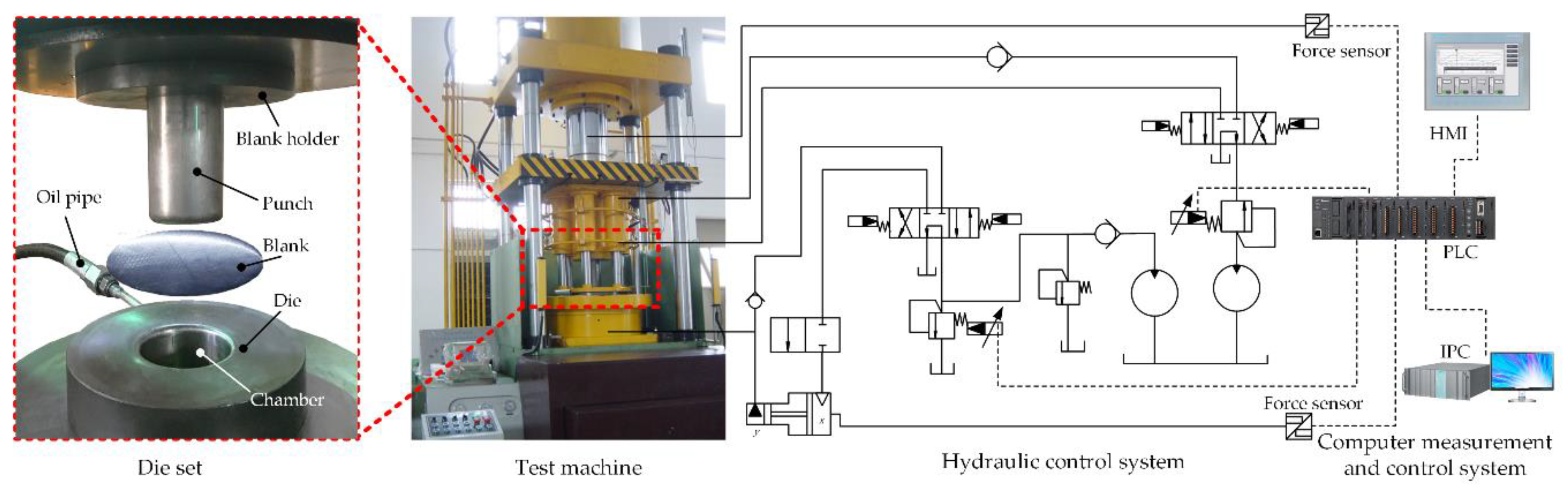
4. Experimental Procedure

4.1. Used Materials

In this study, two different types of aluminum alloy sheets, including 2024-O with a thickness of 1.2 mm and 5754-O with a thickness of 0.9 mm, were implemented to investigate the sheet metal HDD process. The chemical compositions of the 2024-O and 5754-O aluminum alloys are revealed in

Table 1. Chemical composition of the used 2024-O and 5754-O aluminum alloys.

Material	Composition (wt. %)
	Cu	Mg	Si	Mn	Zr	Fe	Ti	Al
2024-O	4.4	1.5	0.5	0.6	-	0.5	0.20	Balance
5754-O	0.1	3.6	0.4	0.5	0.20	0.4	0.15	Balance

.

To determine the mechanical properties and the experimental data needed to obtain the anisotropy coefficients, uniaxial tension tests were performed at seven different angles including 0°, 15°, 30°, 45°, 60°, 75°, and 90° from the rolling direction. An MTS-E43.104 electronic universal testing machine was used to conduct the tensile tests with a tensile strain rate of 1.0 × 10⁻³ s⁻¹. To calibrate the Yld2000-2d and BBC2005 yield functions, equi-biaxial tension tests were also performed on a planar biaxial tension testing machine using cruciform specimens [33]. The experiments were performed three times and the average value was taken for development of the yield criteria. The material characteristic coefficients obtained from experiments are presented in

Table 2. Material characteristic coefficients obtained from tension tests.

Material	${\mathit{\sigma }}_0\left(\mathbf{MPa}\right)$	${\mathit{r}}_{45}\left(\mathbf{MPa}\right)$	${\mathit{r}}_{90}\left(\mathbf{MPa}\right)$	${\mathit{r}}_{\mathbf{b}}\left(\mathbf{MPa}\right)$	${\mathit{r}}_0$	${\mathit{r}}_{45}$	${\mathit{r}}_{90}$	${\mathit{r}}_{\mathbf{b}}$	K	n
2024-O	79.51	75.98	77.71	79.88	0.643	0.939	0.545	0.851	289.34	0.183
5754-O	108.67	108.68	113.39	114.37	0.707	0.894	0.956	1.379	403.24	0.254

.

4.2. Experimental Procedure

The hydrodynamic deep drawing experiments were conducted on double-action specified HDD equipment with a forming capacity of 3500 kN and the maximum blank holder force of 2000 kN. The fluid pressure in die cavity and blank holder force can be regulated in real time according to various designed loading paths controlled by proportional pressure valves, and the maximum cavity pressure can reach 100 MPa. Figure 5. illustrates the die sets of the sheet metal HDD process and the composition of experimental equipment including the test machine, hydraulic control system and computer measurement and control system. The tool geometry is specified in

Table 3. Tools geometry of hydrodynamic deep drawing.

Tool Geometry	Unit (mm)
Punch diameter	50.46
Punch profile radius	5.0
Die opening diameter	53.64
Die profile radius	8.0
Blank holder opening diameter	51.44
Blank holder profile radius	6.0
Blank diameter	93.2

. During the HDD process, pre-bulging pressure was applied on the blank, and a backward bulging was produced. Subsequently, the blank was drawn into the die chamber with the movement of the punch to a desired depth at a constant velocity of 15 mm/min. Meanwhile, the cavity pressure was adjusted by the proportional valve to press the workpiece onto the punch surface and avoid the defects of rupturing and wrinkling.

4.3. Calibration of Anisotropy Coefficient

The anisotropy coefficients of two type Hill’48 yield functions can be calibrated with experimental data. In addition, the eight measured material data were applied to calculate the coefficients of Yld2000-2d yield function. The anisotropy coefficients for BBC2005 function were determined implementing MATLAB R2018b software and optimizing an error function with the Levenberg–Marquardt algorithm. The materials’ anisotropy coefficients for yield criteria are summarized in

Table 4. The anisotropy coefficients of diverse yield functions.

Yield Functions	Materials	Anisotropic Coefficients
Hill’48-R	AA2024-O	F	G	H	N
		0.7174	0.6088	0.3912	1.9079
	AA5754-O	F	G	H	N
		0.4332	0.5858	0.4142	1.4206
Hill’48-S	AA2024-O	F	G	H	N
		0.5189	0.4720	0.5281	1.6948
	AA5754-O	F	G	H	N
		0.4460	0.5275	0.4725	1.5129
Yld2000-2d	AA2024-O	β1	β2	β3	β4
		0.9549	0.9714	0.9427	1.0338
		β5	β6	β7	β8
		1.0089	0.9427	1.0332	1.1222
	AA5754-O	β1	β2	β3	β4
		0.9865	0.9299	0.9019	0.9509
		β5	β6	β7	β8
		0.9952	0.9019	0.9828	1.0809
BBC2005	AA2024-O	a	b	${\kappa }_1$	${\kappa }_2$
		1.2669	0.6482	0.4708	0.4983
		${\kappa }_3$	${\kappa }_4$	${\kappa }_5$	${\kappa }_6$
		0.4143	0.4818	0.4402	0.4416
	AA5754-O	a	b	${\kappa }_1$	${\kappa }_2$
		0.7505	0.5076	0.4145	0.464
		${\kappa }_3$	${\kappa }_4$	${\kappa }_5$	${\kappa }_6$
		0.5306	0.5025	0.5051	0.4734

.

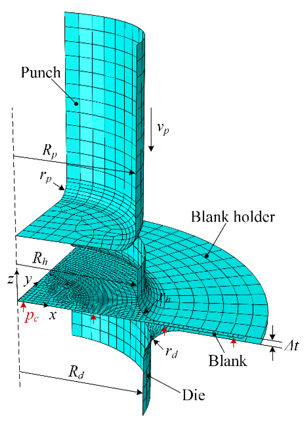
5. Numerical Simulation

In this study, numerical simulations of the sheet metal HDD process were performed utilizing ABAQUS 6.13 software. In addition, for comparison purposes, the Hill’48 yield function, available in the library of ABAQUS software, the Yld2000-2d and BBC2005 yield functions, developed by VUMAT subroutine, were implemented in separate simulations. Due to the orthotropic material properties of aluminum alloy sheets, only a quarter section of the workpiece with the corresponding symmetry boundary conditions was considered. The tooling components were modeled as analytical rigid bodies with the four-node shell. A total of 2560 shell elements with reduced integration (ABAQUS S4R) and five section points through the sheet thickness were applied for the simulation. The contact condition in the tangential direction was governed by the Coulomb friction model. The friction coefficients at the blank/die, blank/blank holder, and blank/punch face interfaces were assumed to be 0.05, 0.08, and 0.1, respectively. Figure 6. demonstrates the dimensions of tooling in the sheet metal HDD process simulation.

6. Results and Discussion

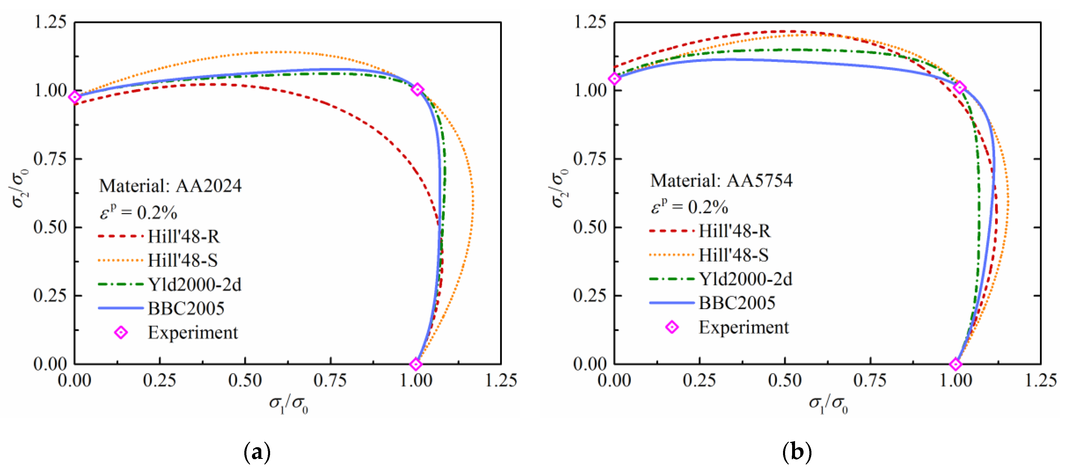
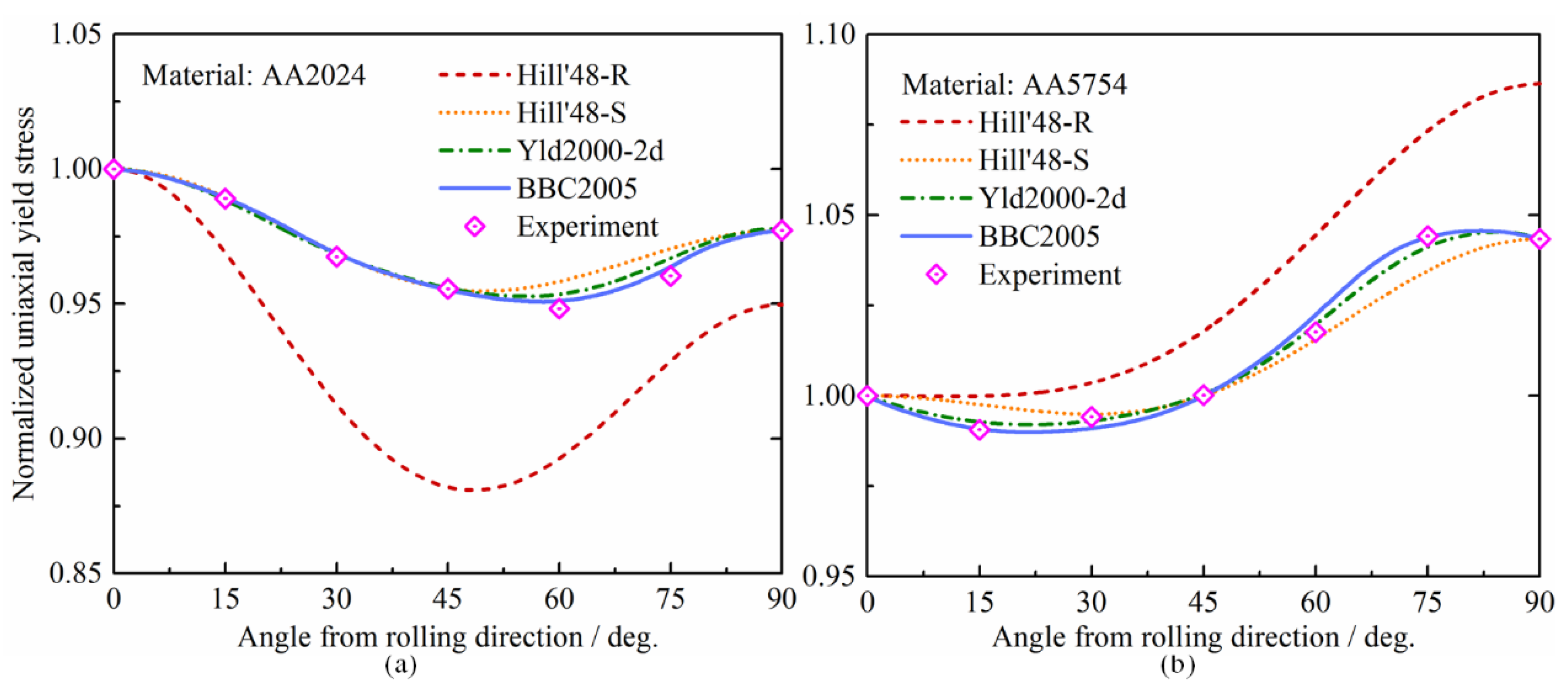
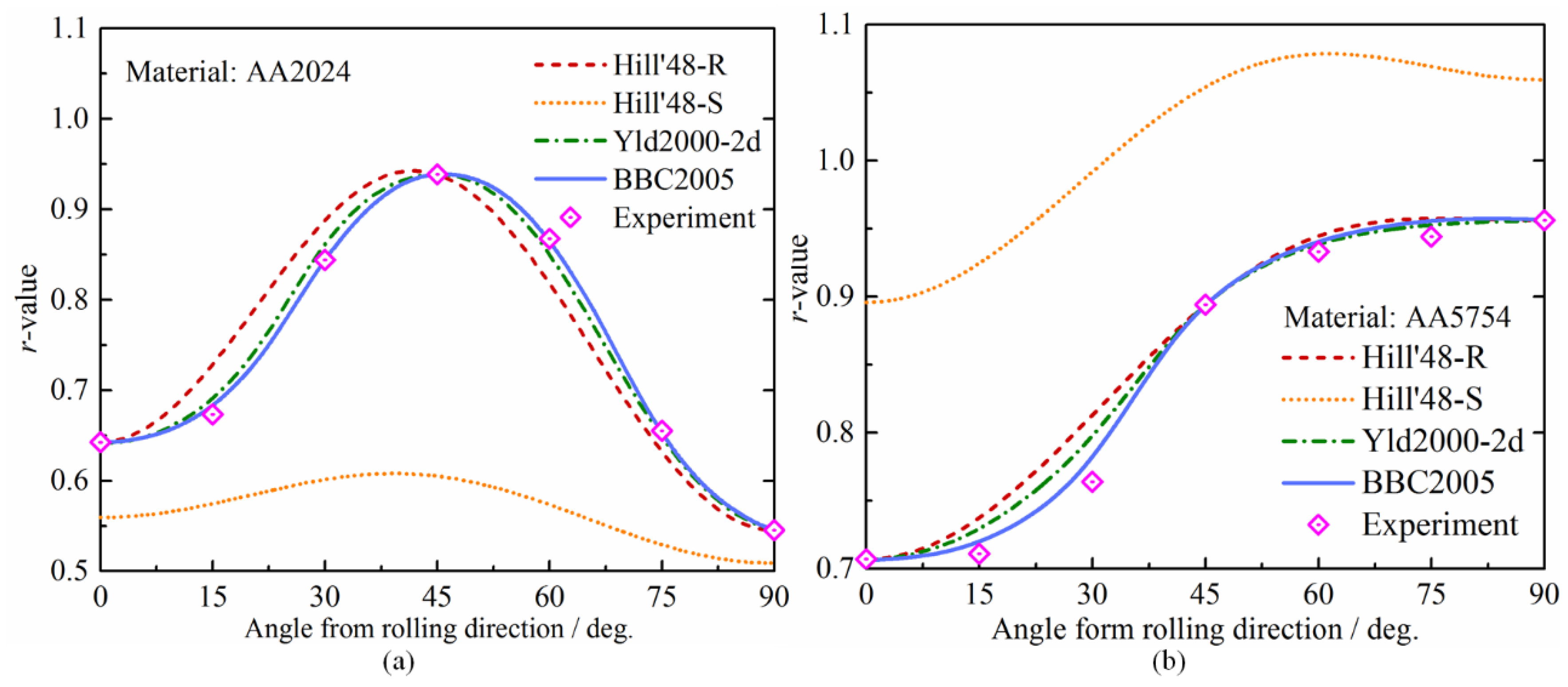
6.1. Effect of Yield Functions on the Prediction of Material Anisotropy

A comparison between experimental consequences and predicted results obtained from diverse anisotropic yield criteria was performed to evaluate the flexibility of the proposed yield functions. The comparison was concentrated on the following performance aspects including prediction of the yield locus geometry and description of the planar distribution both for uniaxial yield stress and uniaxial coefficient of plastic anisotropy (r value).

In Figure 7, the yield locus projected on the zero-shear stress plane for Hill’48-R, Hill’48-S, Yld2000-2d, and BBC2005 anisotropic yield functions of AA2024 and AA5754 are illustrated together with experimental results. The tensile stresses were normalized with the uniaxial stress at rolling direction. For both the AA2024 and the AA5754 cases, predictions of the yield surface provided by BBC2005 and Yld2000-2d models were very similar, while the performances of the Hill’48 models signify differences to the others, being a little smoother in the region around equi-biaxial tension for both cases. This was because the Hill’48 yield function was less flexible than the others due to the fact that it does not include the equi-biaxial stress in its model.

The normalized yield stresses under uniaxial tension along various loading directions were predicted by diverse yield functions for the AA2024 and AA5754 sheet in Figure 8. and compared with the experimental data points. It was found that the results of the yield functions (i.e., Hill’48-S, Yld2000-2d, and BBC2005 models) matched well with that of the experimental data, while the Hill’48-R model underestimated the uniaxial yield stress for AA2024 and overestimated for the AA5754’s in all directions. Moreover, it was apparent that the BBC2005 and Yld2000-2d criteria had better performances in the prediction of the yield stress for both cases. Since the Hill’48-S model was obtained based on the yield stresses, the predicted distribution fit exactly the experimental distribution. Whereas, the predictions based on Hill’48-R criterion were in poorer agreement with the experimental data for both materials.

The uniaxial anisotropy coefficient distributions in the plane of the AA2024 and AA5754 sheets, predicted utilizing different yield criteria, are presented in Figure 9. For the AA2024 case, as demonstrated in Figure 9a, the planar distribution of the r value predicted by Hill’48-S yield criterion was very inaccurate. In contrast, the variation of the r value described by Hill’48-R, Yld2000-2d and BBC2005 models closely followed the experimental results of AA2024 and AA5754. The BBC2005 function provided a slightly better prediction for the r value than the Yld2000-2d function. Concerning AA5754, it was revealed from Figure 9b that the highest r value was at the transverse direction, while the lowest value was at the rolling direction. It can be seen that the predictions for the r value from the BBC2005 yield function matched the experimental results for every orientation very well, with a slight deviation at 75°. The prediction of the r value for Hill’48-S yield function at every 15° from the rolling direction was not as good as the other yield functions because the coefficients for the Hill’48-S model were designed to fit yield stresses at 0°, 45°, and 90°.

The virtual uniaxial tension tests showed that the r values varied in the range of 0.545 to 0.939 and 0.707 to 0.956, while normalized yield stress varied in the range of 0.948 to 1.000 and 0.991 to 1.044 for both materials, i.e., both aluminum alloys revealed strong deformation anisotropy but weak strength anisotropy. Furthermore, the yield stress and r value predicted by the Yld2000-2d and BBC2005 models had better conformity with the experimental results in comparison with the predicted results using the Hill’48 model. It was concluded that the more parameters there were in the Yld2000-2d and BBC2005 yield criteria, the more precisely predicted yield stresses and r values could be obtained.

To have a comprehensive evaluation tool of the anisotropic models, a global accuracy index was developed as follow in Equation (45):

$$\xi ={\xi }_Y+{\xi }_S+{\xi }_R[\%]$$

(45)

where ${\xi }_Y$ is the accuracy index associated to the prediction of the yield locus shape in the plane of the principal stresses; ${\xi }_S$ is the accuracy index associated to the prediction of the planar distribution of the uniaxial yield stress; ${\xi }_R$ is the accuracy index associated to the prediction of the planar distribution of the uniaxial coefficient of plastic anisotropy. ${\xi }_Y$, ${\xi }_S$, and ${\xi }_R$ are computed using the following formulas:

$$\{\begin{array}{l}{\xi }_Y={\displaystyle \sum _{i=1}^n\frac{d_i}{n\cdot \sqrt{{\left({\sigma }_1^i\right)}^2+{\left({\sigma }_2^i\right)}^2}}}100[\%]\\ {\xi }_S={\displaystyle \sum _{i=1}^n\left|\frac{{\sigma }_{{\theta }_i}^{\exp }-{\sigma }_{{\theta }_i}^t}{n\cdot {\sigma }_{{\theta }_i}^{\exp }}\right|}100[\%]\\ {\xi }_R={\displaystyle \sum _{i=1}^n\left|\frac{r_{{\theta }_i}^{\exp }-r_{{\theta }_i}^t}{n\cdot r_{{\theta }_i}^{\exp }}\right|100[\%]}\end{array}$$

(46)

where d_i is the squared distance from an experimental point to the yield locus predicted by the yield criterion under testing; n is the total number of the available experimental points; ${\sigma }_{{\theta }_i}^{exp}$ is the experimental uniaxial yield stress corresponding to the direction defined by the angle θ_i (measured from the rolling direction); ${\sigma }_{{\theta }_i}^t$ is the predicted uniaxial yield stress associated to the same direction; $r_{{\theta }_i}^{exp}$ is the experimental anisotropy coefficient corresponding to the direction defined by the angle θ_i (measured from the rolling direction); $r_{{\theta }_i}^t$ is the predicted anisotropy coefficient corresponding to the same direction.

The values of the individual accuracy indexes are shown in Figure 10. The best overall performance corresponded to the lowest value of the global yield criterion accuracy index $\xi$. It was revealed that the values of the anisotropic accuracy index of the Yld2000-2d and BBC2005 yield criteria for both materials were lower than the values for the two Hill’48 yield criteria. This demonstrates the higher reliability of the Yld2000-2d and BBC2005 yield functions rather than the other ones for both aluminum alloys.

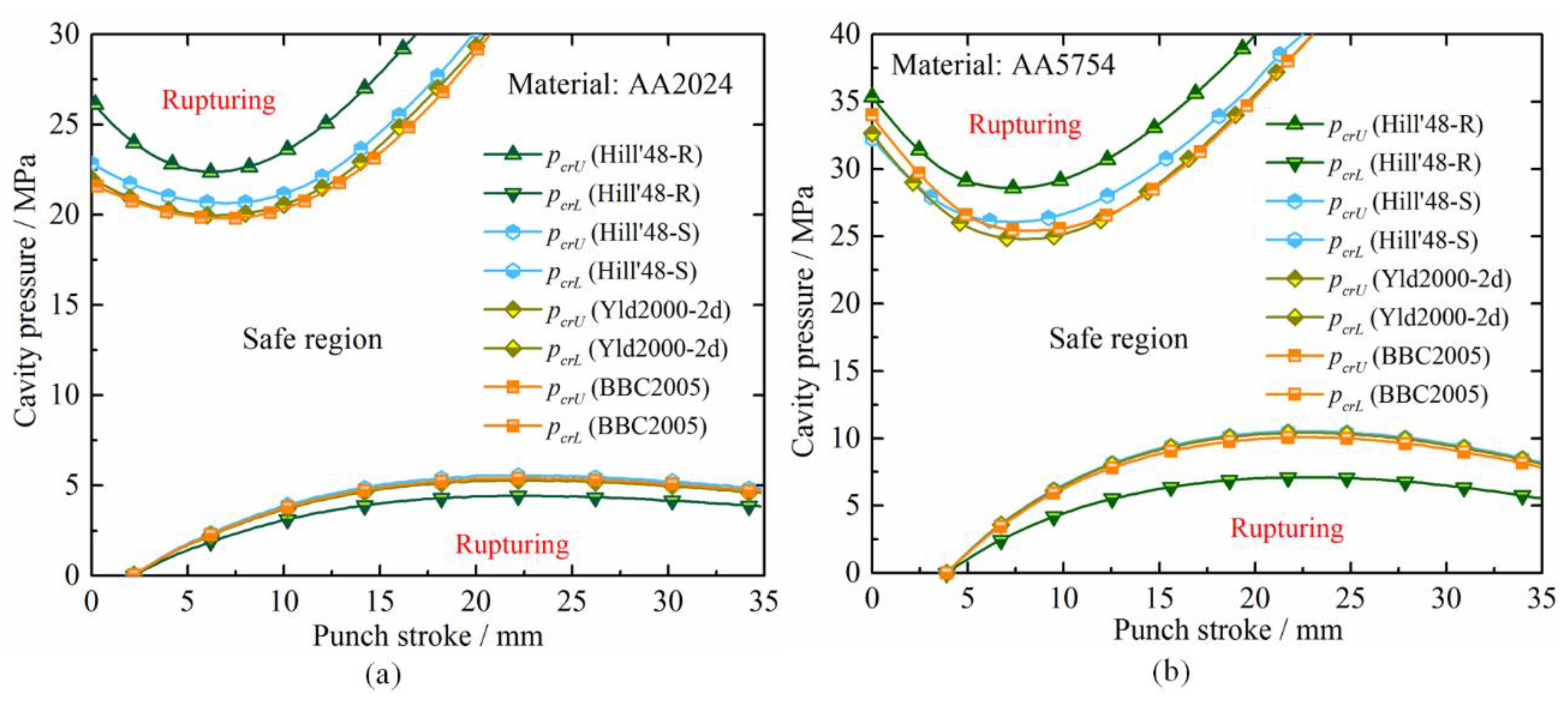
6.2. The Adaptability of Yield Functions to Predict the Critical Process Window

The critical process window of cavity pressure can be acquired by calculating the lower and upper critical pressures utilizing the analytical procedure, illustrated in Figure 4, together with the material properties and the geometrical dimensions of the workpiece. The relationship between the reasonable cavity pressure and the punch stroke during the HDD process is a significant challenge. On the one hand, the material is bent to the radius of curvature of the punch much faster than the allowed ductility of the material when the pressure is higher than the upper critical pressure curve, which might lead to the rupture of the workpiece around the die shoulder. On the other hand, the material flow resistance is increased, and the sheet is unable to be entirely separated from the die radius if the cavity pressure is smaller than the lower critical pressure. In turn, the sharp thinning around the punch radius is increased which also results in the rupture of the part. Consequently, the safe area between the upper and lower critical profiles can provide reasonable cavity pressure versus punch stroke locus to ensure a flawless part. The critical upper and lower pressure curves predicted based on the Hill’48-R, Hill’48-S, Yld2000-2d, and BBC2005 yield criteria for both materials are illustrated in Figure 11. in which critical pressures in respect to the punch stroke are drawn. It was revealed that the critical pressure loading window predicted by the Hill’48-S, Yld2000-2d, and BBC2005 yield criteria was approximately the same, while the safety area in the critical process window predicted by the Hill48-R yield criteria was greater than the predictions of the other three criteria’s results.

To explore the adaptability of yield functions to predict the critical process window of cylindrical part, several loading loci were designed for hydroforming experiment for AA2024 and AA5754, respectively, as revealed in Figure 12a,b. Moreover, the maximum wall thickness reduction ratio for the fabricated workpieces are measured to evaluate the critical process window of cavity pressure, as depicted in Figure 13a,b. It can be observed that excessive or insufficient cavity pressure induced the severe thinning around the punch radius region in the results of Locus A and Locus B in Figure 12. and Locus A in Figure 13. For the loading Loci A and B, ruptures appeared because the cavity pressures were too low to entirely separate the blank from the die orifice at the beginning of hydroforming process. On the other hand, for the loading locus J, apparent thickness reduction and fracture are occurred before the blank thoroughly coated with the punch due to the excessive pressure, which is not conducive to the subsequent forming. It is demonstrated that the Locus A in Figure 10 is lower than the lower critical loci of all the yield criteria in Figure 9a. Although the Locus B is in the safe region predicted by Hill’48-R model, it crosses the lower limit of the loading path predicted by the other three yield criteria. Moreover, the Locus J is higher than the upper limit of all yield criteria in Figure 9a. Although the path I is in the safe area predicted by Hill’48-R, it has an intersection with the lower critical pressure locus predicted by the other three yield criteria. It can be seen from Figure 11 that the same situation also occurred in the investigation of AA5754.

Figure 14. compares the experimental critical pressure loading loci with those predicted by the four yield criteria for both aluminum alloys. It can be clearly observed that the critical pressure curves predicted by the Hill’48-R, Hill’48-S, Yld2000-2d and BBC2005 models all had proper conformity with the experimental results, but the Hill’48-R model predicted a larger safe region than the Yld2000-2d and BBC2005 models. To be more specific, the predictions of the Hill’48-S, Yld2000-2d, and BBC2005 criteria were much closer to the experimental safe region for both the AA2024 and AA5754 alloys. Therefore, it can be proved that the Hill48-S, Yld2000-2d, and BBC2005 models were more accurate than the Hill48-R model in predicting the critical process window of the aluminum alloy sheet metal HDD process.

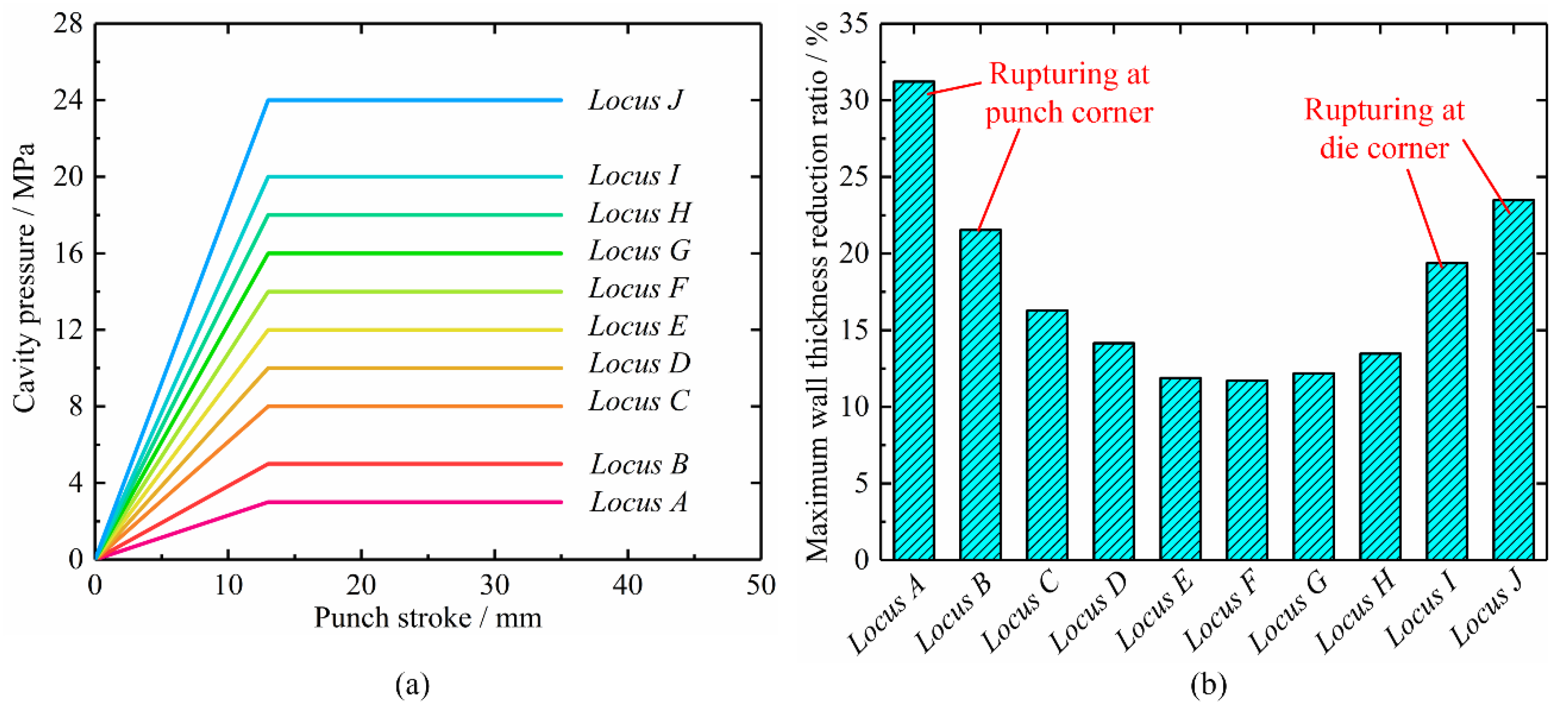
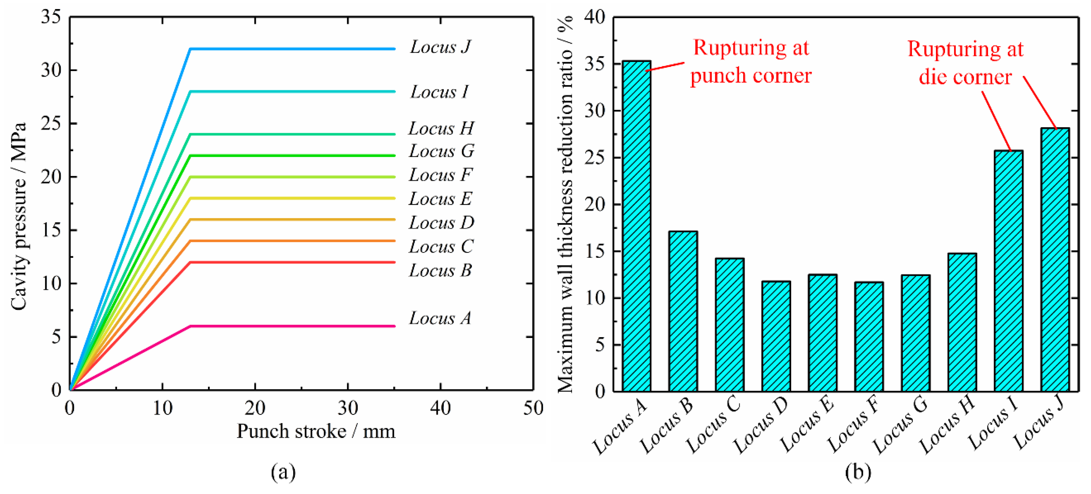
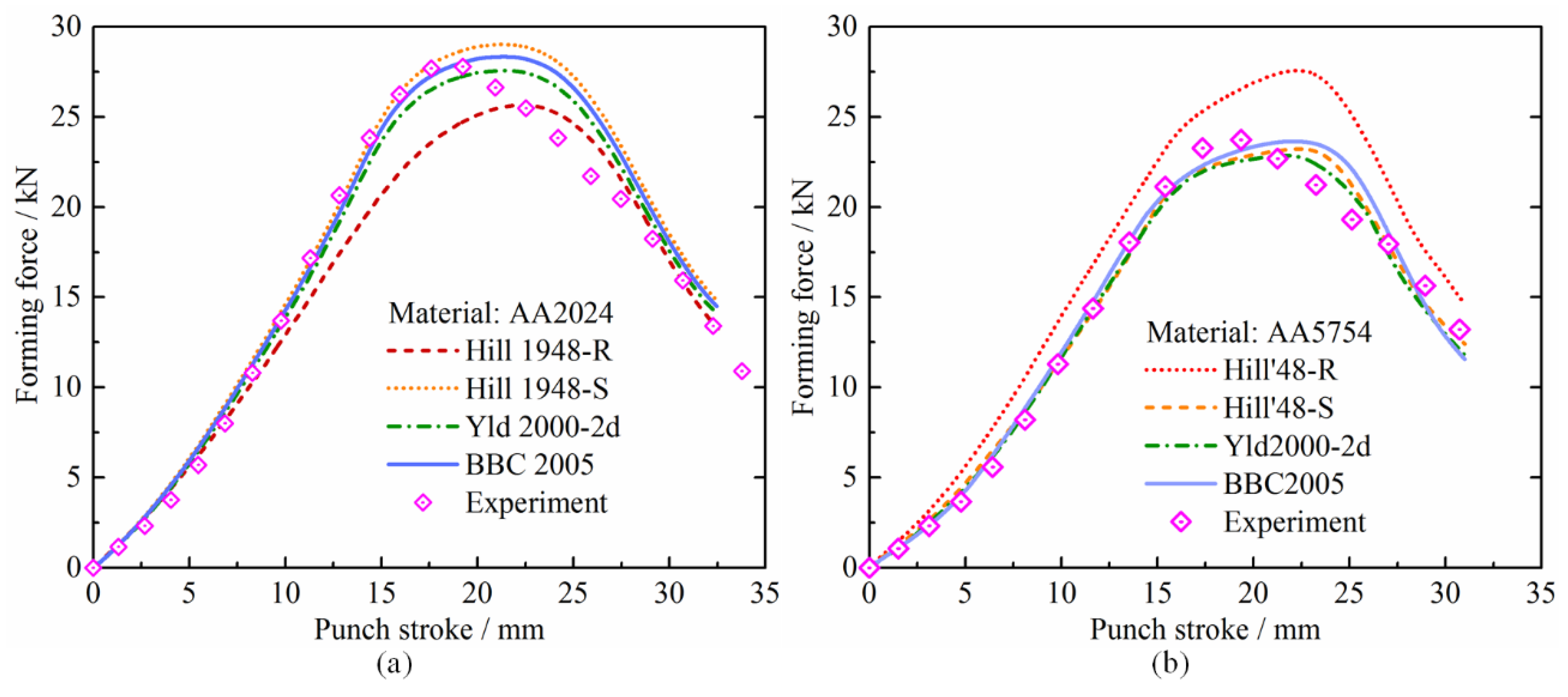
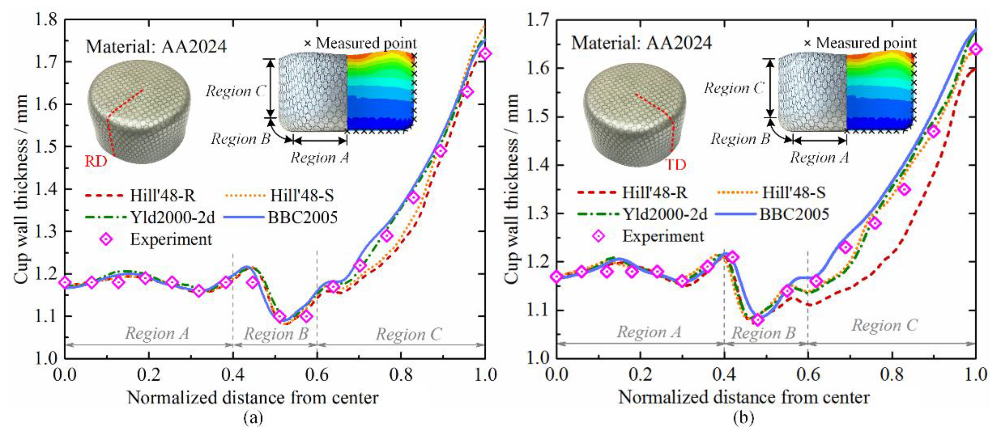
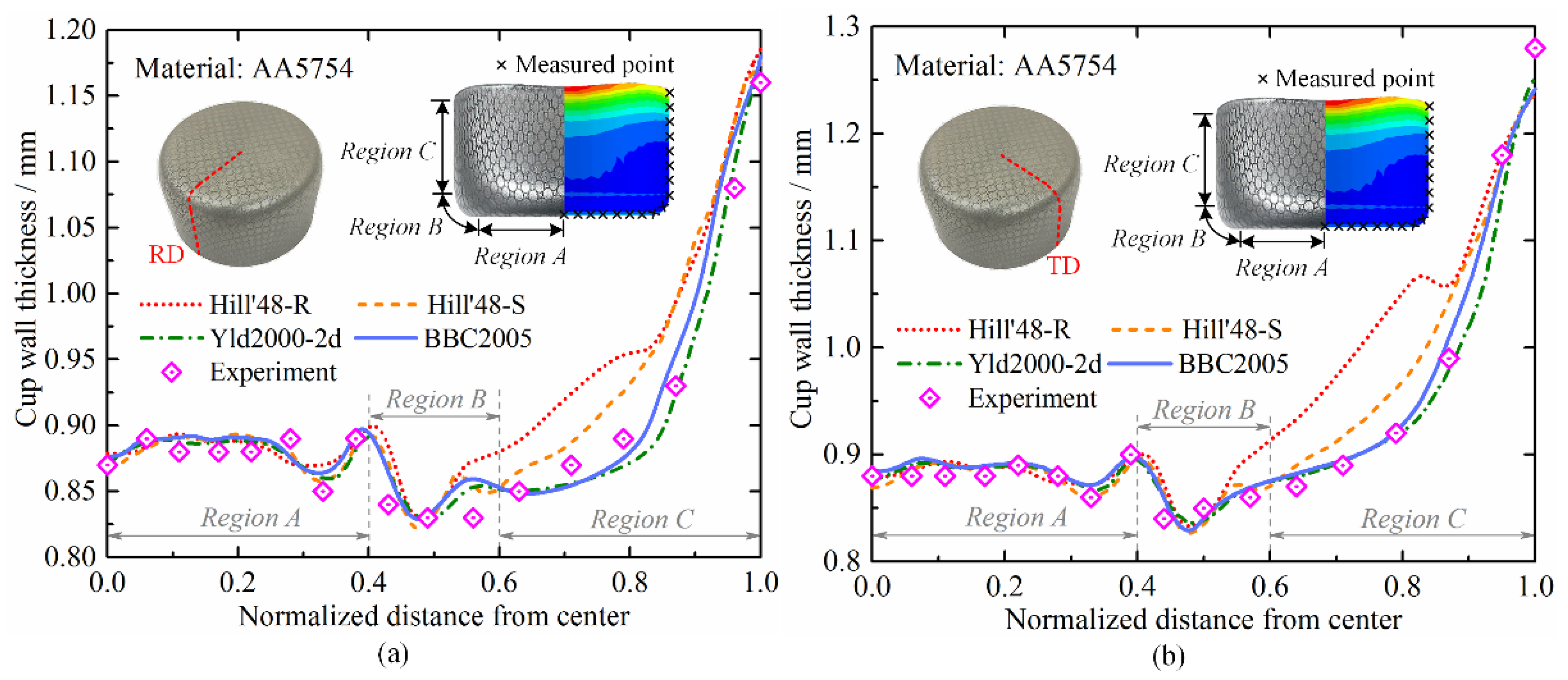
6.3. Effect of Yield Functions on the Prediction Accuracy of Deformation Behavior

The comparison between experimental and numerical punch force evolution during the hydroforming process of AA2024 and AA5754 are displayed in Figure 15. The punch force was a global variable and, therefore, was roughly insensitive to the yield criteria with the range between the lower and upper punch force predictions reaching approximately 20% for both materials.

For the 2024 aluminum alloy, the experimental evolution was accurately predicted by the Hill’48-S, Yld2000-2d and BBC2005 models. However, the Hill’48-R yield criterion underestimated the necessary punch force required for further drawing after 10 mm, although the slope was correctly predicted. Concerning the AA5754, the punch force evolution obtained with the BBC2005 yield model, which seem to be closer to the experimental one, was located among the results achieved with the Hill’48 yield criteria, utilizing the two approaches for material parameters identification. Moreover, the Hill’48-S and Yld2000-2d models led to similar results in terms of punch force evolution. The punch force predicted by the Hill’48-R model was higher than applying other three models.

The earing profile is defined by the height of the drawn cup measured along the circumferential direction of the cup using the angle with the rolling direction. A comparison of the experimental earing profile with the computationally predicted earing profiles is featured in Figure 16. It can be stated that the earing profile predicted by the BBC2005 and Yld2000-2d models was in rather good qualitative agreement with experiments for AA2024 and AA5754. Although the two calibrated forms of Hill’48 yield criterion could predict the locations of the peaks and valleys, the earing profiles were overestimated by Hill’48-R, underestimated by Hill’48-S for AA2024, and overestimated by Hill’48-S for AA5754. The earing profile was poorly predicted by the Hill’48 yield model. On the other hand, the Yld2000-2d function predicted the earing profile but not as precisely as the earing predicted by the BBC2005 yield model which is evident from Figure 16.

The capability and accuracy of the selected yield functions in the prediction of thickness variations in the HDD process were investigated. The wall thickness variations obtained by simulation at the rolling and the transverse directions were measured and compared with the corresponding experimental results in three different regions of AA2024 and AA5754 as plotted in Figure 17 and Figure 18, respectively. Based on the simulation results for AA2024, shown in Figure 17, predictions of thickness variation at the rolling and the transverse directions were nearly the same for all yield criteria and approximately coincided with the experimental results. Moreover, it was observed that the simulation results based on the Yld2000-2d and BBC2005 yield functions were in better agreement with the experimental results for both aluminum alloys than those based on the other three yield functions. Concerning the consequences for the AA5754 alloy in Figure 18, the wall thickness in Region C was overestimated by the Hill’48-R function in both directions.

7. Conclusions

In this research, three anisotropic yield criteria including Hill’48, Yld2000-2d, and BBC2005 were implemented to describe the anisotropic behavior in the hydrodynamic deep drawing process of aluminum alloys. Theoretical models based on different yield criteria were developed to determine the critical pressure at instability points and the critical process window in the HDD process of cylindrical cups. Furthermore, the accuracy of the predicted materials’ anisotropic coefficients was evaluated by the experimental results. The effect of the anisotropic yield criterion on the prediction of the critical process window and material deformation behavior in the HDD process was investigated. The conclusions have been drawn as follows:

(1) The Yld2000-2d and BBC2005 yield formulas performed better in predicting the anisotropic coefficients, yield locus, and directional flow stresses for the AA2024 and AA5754 alloys. However, the Hill’48 yield function provided relatively poor capability in the prediction of the r value and uniaxial yield stress due to the fact that it underestimated the biaxial yield stress for aluminum alloys.

(2) Although all of the four anisotropic yield models had proper conformity with the experimental results of the critical process window, the predictions using the Yld2000-2d and BBC2005 yield criteria were much closer to the experimental safe region for both the AA2024 and AA5754 alloys.

(3) The FEM results based on the Yld2000-2d and BBC2005 yield functions were in closer agreement with experimental data in terms of forming load, cup earing height, and wall thickness distribution for both AA2024 and AA5754 alloys. The flexible yield functions, like BBC2005 and Yld2000-2d, with more anisotropic parameters provided better predictability in modeling the critical process window and anisotropic deformation in the HDD process of aluminum alloys.

References

1. Dursun, T.; Soutis, C. Recent developments in advanced aircraft aluminium alloys. Mater. Des. 2014, 56, 862–871. [Google Scholar] [CrossRef]
2. Zhang, S.H.; Jensen, M.R.; Danckert, J.; Nielsen, K.B.; Kang, D.C.; Lang, L.H. Analysis of the hydromechanical deep drawing of cylindrical cups. J. Mater. Process. Technol. 2000, 103, 367–373. [Google Scholar] [CrossRef]
3. Jalil, A.; Hoseinpour, G.M.; Sheikhi, M.M.; Seyedkashi, S.M.H. Hydrodynamic deep drawing of double layered conical cups. Trans. Nonferr. Met. Soc. China 2016, 26, 237–247. [Google Scholar] [CrossRef]
4. Meng, B.; Wan, M.; Wu, X.; Yuan, S.; Xu, X. Inner wrinkling control in hydrodynamic deep drawing of an irregular surface part using drawbeads. Chinese. J. Aeronaut. 2014, 27, 697–707. [Google Scholar] [CrossRef] [Green Version]
5. Halkaci, H.S.; Turkoz, M.; Dilmec, M. Enhancing formability in hydromechanical deep drawing process adding a shallow drawbead to the blank holder. J. Mater. Process. Technol. 2014, 214, 1638–1646. [Google Scholar] [CrossRef]
6. Singh, S.K.; Kumar, D.R. Effect of process parameters on product surface finish and thickness variation in hydro-mechanical deep drawing. J. Mater. Process. Technol. 2008, 204, 169–178. [Google Scholar] [CrossRef]
7. Meng, B.; Wan, M.; Yuan, S.; Xu, X.; Liu, J.; Huang, Z. Influence of cavity pressure on hydrodynamic deep drawing of aluminum alloy rectangular box with wide flange. Int. J. Mech. Sci. 2013, 77, 217–226. [Google Scholar] [CrossRef]
8. Bagherzadeh, S.; Mirnia, M.J.; Mollaei Dariani, B. Numerical and experimental investigations of hydro-mechanical deep drawing process of laminated aluminum/steel sheets. J. Manuf. Process. 2015, 18, 131–140. [Google Scholar] [CrossRef]
9. Wang, C.; Wan, M.; Meng, B.; Xu, L. Process window calculation and pressure locus optimization in hydroforming of conical box with double concave cavities. Int. J. Adv. Manuf. Technol. 2016, 91, 847–858. [Google Scholar] [CrossRef]
10. Zhang, F.; Li, X.; Xu, Y.; Chen, J.; Chen, J.; Liu, G.; Yuan, S. Simulating sheet metal double-sided hydroforming by using thick shell element. J. Mater. Process. Technol. 2015, 221, 13–20. [Google Scholar] [CrossRef]
11. Yaghoobi, A.; Baseri, H.; Jooybari, M.B.; Gorji, H. Pressure path optimization of hydrodynamic deep drawing of cylindrical-conical parts. Int. J. Precis. Eng. Manuf. 2013, 14, 2095–2100. [Google Scholar] [CrossRef]
12. Li, W.D.; Meng, B.; Wang, C.; Wan, M.; Xu, L. Effect of pre-forming and pressure path on deformation behavior in multi-pass hydrodynamic deep drawing process. Int. J. Mech. Sci. 2017, 121, 171–180. [Google Scholar] [CrossRef]
13. Zampaloni, M.; Abedrabbo, N.; Pourboghrat, F. Experimental and numerical study of stamp hydroforming of sheet metals. Int. J. Mech. Sci. 2003, 45, 1815–1848. [Google Scholar] [CrossRef]
14. Liu, B.; Lang, L.; Zeng, Y.; Lin, J. Forming characteristic of sheet hydroforming under the influence of through-thickness normal stress. J. Mater. Process. Technol. 2012, 212, 1875–1884. [Google Scholar] [CrossRef]
15. Lang, L.; Li, T.; Zhou, X.; Kristensen, B.E.; Danckert, J.; Nielsen, K.B. Optimized decision of the exact material modes in the simulation for the innovative sheet hydroforming method. J. Mater. Process. Technol. 2006, 177, 692–696. [Google Scholar] [CrossRef]
16. Gorji, A.; Alavi-Hashemi, H.; Bakhshi-jooybari, M.; Nourouzi, S.; Hosseinipour, S.J. Investigation of hydrodynamic deep drawing for conical-cylindrical cups. Int. J. Adv. Manuf. Technol. 2011, 56, 915–927. [Google Scholar] [CrossRef]
17. Neto, D.M.; Oliveira, M.C.; Alves, J.L.; Menezes, L.F. Influence of the plastic anisotropy modelling in the reverse deep drawing process simulation. Mater. Des. 2014, 60, 368–379. [Google Scholar] [CrossRef]
18. Izadpanah, S.; Ghaderi, S.H.; Gerdooei, M. Material parameters identification procedure for BBC2003 yield criterion and earing prediction in deep drawing. Int. J. Mech. Sci. 2016, 115–116, 552–563. [Google Scholar] [CrossRef]
19. Soare, S.C.; Barlat, F. A study of the Yld2004 yield function and one extension in polynomial form: A new implementation algorithm, modeling range, and earing predictions for aluminum alloy sheets. Eur. J. Mech. A Solids 2011, 30, 807–819. [Google Scholar] [CrossRef]
20. Wang, L.; Lee, T.C. The effect of yield criteria on the forming limit curve prediction and the deep drawing process simulation. Int. J. Mach. Tool. Manuf. 2006, 46, 988–995. [Google Scholar] [CrossRef]
21. Lang, L.H.; Li, T.; Zhou, X.B.; Kristensen, B.E.; Danckert, J.; Nielsen, K.B. Optimized constitutive equation of material property based on inverse modeling for aluminum alloy hydroforming simulation. Trans. Nonferr. Met. Soc. China 2006, 16, 1379–1385. [Google Scholar] [CrossRef]
22. Kotkunde, N.; Deole, A.D.; Gupta, A.K.; Singh, S.K. Experimental and numerical investigation of anisotropic yield criteria for warm deep drawing of Ti–6Al–4V alloy. Mater. Des. 2014, 63, 336–344. [Google Scholar] [CrossRef]
23. Cai, Z.; Diao, K.; Wu, X.; Wan, M. Constitutive modeling of evolving plasticity in high strength steel sheets. Int. J. Mech. Sci. 2016, 107, 43–57. [Google Scholar] [CrossRef]
24. Khalfallah, A.; Alves, J.L.; Oliveira, M.C.; Menezes, L.F. Influence of the characteristics of the experimental data set used to identify anisotropy parameters. Simul. Model. Pract. Theory 2015, 53, 15–44. [Google Scholar] [CrossRef] [Green Version]
25. Hashemi, A.; Hoseinpour, G.M.; SEYEDKASHI, S.M.H. Process window diagram of conical cups in hydrodynamic deep drawing assisted by radial pressure. Trans. Nonferr. Met. Soc. China 2015, 25, 3064–3071. [Google Scholar] [CrossRef]
26. Azodi, H.D.; Naeini, H.M.; Parsa, M.H.; Liaghat, G.H. Analysis of rupture instability in the hydromechanical deep drawing of cylindrical cups. Int. J. Adv. Manuf. Technol. 2008, 39, 734–743. [Google Scholar] [CrossRef]
27. Banabic, D.; Barlat, F.; Cazacu, O.; Kuwabara, T. Advances in anisotropy and formability. Int. J. Mater. Form. 2010, 3, 165–189. [Google Scholar] [CrossRef]
28. Yoon, J.W.; Dick, R.E.; Barlat, F. A new analytical theory for earing generated from anisotropic plasticity. Int. J. Plast. 2011, 27, 1165–1184. [Google Scholar] [CrossRef]
29. Hill, R. A Theory of the Yielding and Plastic Flow of Anisotropic Metals. Proceedings A 1948, 193, 281–297. [Google Scholar] [CrossRef] [Green Version]
30. Barlat, F.; Brem, J.C.; Yoon, J.W.; Chung, K.; Dick, R.E.; Lege, D.J.; Pourboghrat, F.; Choi, S.-H.; Chu, E. Plane stress yield function for aluminum alloy sheets—Part 1: Theory. Int. J. Plast. 2003, 19, 1297–1319. [Google Scholar] [CrossRef]
31. Banabic, D. An improved analytical description of orthotropy in metallic sheets. Int. J. Plast. 2005, 21, 493–512. [Google Scholar] [CrossRef]
32. Bagherzadeh, S.; Mollaei-Dariani, B.; Malekzadeh, K. Theoretical study on hydro-mechanical deep drawing process of bimetallic sheets and experimental observations. J. Mater. Process. Technol. 2012, 212, 1840–1849. [Google Scholar] [CrossRef]
33. Wang, H.B.; Wan, M.; Wu, X.D.; Yan, Y. Subsequent yield loci of 5754O aluminum alloy sheet. Trans. Nonferr. Met. Soc. China 2009, 19, 1076–1080. [Google Scholar] [CrossRef]
Figure 1. A schematic of the sheet metal hydrodynamic deep drawing (HDD) process.
Metals 10 00492 g001
Figure 2. Comparison of the conventional deep drawing process and HDD process.
Metals 10 00492 g002
Figure 3. Stress model of workpiece in the sheet metal HDD process.
Metals 10 00492 g003
Figure 4. Calculation procedures for the critical process window for the sheet metal HDD process.
Metals 10 00492 g004
Figure 5. Experimental setup of hydrodynamic deep drawing process.
Metals 10 00492 g005
Figure 6. Finite element analysis model of the sheet metal HDD process.
Metals 10 00492 g006
Figure 7. Comparison between experimental and predicted yield surface shapes by four yield criteria for (a) AA2024-O and (b) AA5754-O.
Metals 10 00492 g007
Figure 8. Comparison between experimental and predicted uniaxial normalized yield stress distribution by four yield criteria for (a) AA2024-O and (b) AA5754-O.
Metals 10 00492 g008
Figure 9. Comparison between experimental and predicted anisotropy coefficient distribution by four yield criteria for (a) AA2024-O and (b) AA5754-O.
Metals 10 00492 g009
Figure 10. Accuracy indexes of different yield criteria for (a) AA2024-O and (b) AA5754-O.
Metals 10 00492 g010
Figure 11. Critical pressure loading loci predicted by various yield functions (a) AA2024 and (b) AA5754. pcrU and pcrL are the upper and lower critical cavity pressure loci, respectively.
Metals 10 00492 g011
Figure 12. Sheet metal hydrodynamic deep drawing experiment of AA2024: (a) various cavity pressure loading loci and (b) maximum wall thickness reduction ratio of the workpiece.
Metals 10 00492 g012
Figure 13. Sheet metal hydrodynamic deep drawing experiment of AA5754: (a) various cavity pressure loading loci and (b) maximum wall thickness reduction ratio of the workpiece.
Metals 10 00492 g013
Figure 14. Comparison of the critical pressure loading loci predicted by various yield functions and experiment for: (a) AA2024 and (b) AA5754.
Metals 10 00492 g014
Figure 15. A comparison of the experimental and numerically simulated punch force versus punch displacement relationship: (a) AA2024 and (b) AA5754.
Metals 10 00492 g015
Figure 16. Earing profile obtained from simulations in comparison to the experimental results: (a) AA2024 and (b) AA5754.
Metals 10 00492 g016
Figure 17. Experimental and numerical thickness distribution in the AA2024 cup wall at (a) rolling direction and (b) transverse direction.
Metals 10 00492 g017
Figure 18. Experimental and numerical thickness distribution in the AA5754 cup wall at (a) rolling direction and (b) transverse direction.
Metals 10 00492 g018