Quantifying Mechanical Properties of Automotive Steels with Deep Learning Based Computer Vision Algorithms

Abstract

This paper demonstrates that the instrumented indentation test (IIT), together with a trained artificial neural network (ANN), has the capability to characterize the mechanical properties of the local parts of a welded steel structure such as a weld nugget or heat affected zone. Aside from force-indentation depth curves generated from the IIT, the profile of the indented surface deformed after the indentation test also has a strong correlation with the materials’ plastic behavior. The profile of the indented surface was used as the training dataset to design an ANN to determine the material parameters of the welded zones. The deformation of the indented surface in three dimensions shown in images were analyzed with the computer vision algorithms and the obtained data were employed to train the ANN for the characterization of the mechanical properties. Moreover, this method was applied to the images taken with a simple light microscope from the surface of a specimen. Therefore, it is possible to quantify the mechanical properties of the automotive steels with the four independent methods: (1) force-indentation depth curve; (2) profile of the indented surface; (3) analyzing of the 3D-measurement image; and (4) evaluation of the images taken by a simple light microscope. The results show that there is a very good agreement between the material parameters obtained from the trained ANN and the experimental uniaxial tensile test. The results present that the mechanical properties of an unknown steel can be determined by only analyzing the images taken from its surface after pushing a simple indenter into its surface.

1. Introduction

Thermal manufacturing processes of high strength steels such as welding or cutting lead to the local deterioration of the mechanical properties [1]. By knowing the local mechanical properties, not only can the full potential of lightweight constructions be exploited, but also important and hardly accessible local stress–strain relations of welded joints can be obtained for the prediction of the strength of the welded components [2].

The instrumented indentation test (IIT) is a well-known semi-destructive method that enables the determination of the mechanical properties [3] of small areas such as welded zones [4]. In general, the indentation response depends on the material mechanical properties such as the stress–strain curve. By correctly analyzing the indentation response, it is possible to predict the causing parameters that cannot be directly calculated [5].

The indentation force and penetration depth are constantly measured during the execution of the IIT to create the force–indentation depth curve. Three main methods have been introduced to evaluate the mechanical tensile properties from the experimentally measured force–indentation depth curve [6]. The first two methods are the representative stress–strain approach based on Tabor’s work [7] and the inverse simulation using the finite element analysis [8]. In the representative stress–strain method, the true stress–strain diagram can be calculated by determining the contact angle, the pile up or sink in [9] height, and the contact area. Numerous experiments [10,11] have proven the robustness of this method for a wide range of materials. In the inverse simulation method, the quality of the numerical simulation results of the indentation test depends on the modeling of the pile up and sink in effect as well as considering the friction between the indenter and substrate [12]. Although it is possible to implement any material model or use a different type of indenter [13], this method is numerically expensive and needs long-standing experience in the field of numerical simulation. Moreover, it is necessary to determine the starting parameters properly and use an additional optimization algorithm to find acceptable material parameters. There is enough experimental evidence [14,15,16,17] to prove the applicability of this method for metals and ceramics.

The other method implemented in this paper is the evaluation of the data by means of an artificial neural network (ANN). The ANN has demonstrated great potential to predict the mechanical properties of the indented surface. Huber et al. successfully determined the Poisson ratio [18,19], the parameters of a viscoplastic material model [20,21], and the strain hardening properties [22,23] from the indentation test. Moreover, there is good agreement between the experimental data and the ANN prediction of the local stress–strain properties of the resistance spot [24] and friction stir welded joints [25]. In addition, the application of an ANN has been widespread in computational mechanics to solve various inverse problems such as the crack growth analysis of welded specimens [26]. Moreover, a method was proposed by Li et al. [27] to characterize the mechanical properties of heterogeneous materials through images taken from a mesoscale structure. In another example, Ye et al. [28] correlated the stress–strain diagrams with the images taken from the complex microstructures of the composites. Xu et al. [29] applied the convolution neural network on images obtained from the chemical composition of hot rolled steel to predict their mechanical properties. Furthermore, Chun et al. [30] predicated the residual strength of the structural steels by visual inspection of the damage and analyzing the taken images with a convolutional neural network (CNN). In another work, Psuj [31] introduced a novel approach for the characterization of defected areas in steel elements. He implemented the material state evaluation model by using a deep CNN.

The works described above demonstrate the application of machine learning in the field of material characterization. In the current research, we would like to present a novel approach to determine the mechanical properties in a more practical way by using less complex equipment and focusing on the macroscale, which can be used easily in the industry.

ANN is one of the machine learning (ML) algorithms inspired by the biological neuronal network in the brain. ML has gained much popularity these days due to its capability to perform specific tasks without modeling the specific problem, instead relying on patterns or trends of the examples [32]. The learning process of ML can be mainly distinguished between the supervised and unsupervised methods. The supervised learning algorithm learns from the training data containing the inputs and desired outputs. The goal of supervised learning is to approximate functional dependency between the input and the output. However, the training data that do not have outputs can be identified based on its pattern by the so-called unsupervised learning approach [33].

ANN is one of the supervised learning algorithms since the output is required in the training procedure. During the training, the ANN adjusts its weights or hidden layers in order to minimize the error between the desired and the calculated output. The hidden layer is located between the input and output layer where artificial neurons receive a series of weighted inputs and produce an output. Furthermore, the weight shows the influence of the neurons on each other. If an input has a greater weight, this means that this input is more important when compared to other inputs. The trained ANN has this ability to predict the output of an unknown input within the training data space, despite the non-linearity and noise in the data. This capability of the ANN is called generalization [34].

Increasing the number of neurons or hidden layers enhances the complexity of the network and has been found to greatly affect the performance of the ANN [35]. Therefore, variables of the training datasets have to be dimensionally reduced without missing any important information. To train an ANN with training data in the form of a curve, the data points in a curve must be given to ANN for the training. The other alternative is to use parameters that define a curve through a function such as material model parameters that define the stress–strain curve.

Furthermore, to identify objects with a large number of variables such as images, deep learning algorithms with CNN can be applied. Within CNN, the images are passed through multiple hidden layers to extract the local features of the image before they are finally identified. A typical CNN consists of convolution layers, pooling layers, and fully connected layers [36]. For instance, by using the images of a steel surface as the training data, a CNN can be trained to classify the steel [37] or detect a surface defect such as cavities on a rail [38]. However, feature extraction with CNN layers requires a handful of labeled images for the training procedure [39]. Another alternative is to use image segmentation as one of the computer vision algorithms. With segmentation, an image is decomposed into multiple parts (segments), which can be more efficiently used for further analysis [40]. Clustering is one of the most common unsupervised methods to perform image segmentation. Within clustering, one can recognize the pattern in large amounts of data and partition them based on its similarity into groups called clusters. Besides image segmentation, clustering is used in many fields of application such as text information classification [41] and mobile data analysis [42]. This approach has been shown to be effective to perform clustering by employing a square error criterion [43].

The basic procedure for training an ANN to determine the mechanical properties of materials is described in [44] and was implemented in this paper. Initially, numerous correlations between the indentation path and the mechanical behavior were required to train the ANN. Therefore, in order to generate data, it is necessary to start with the numerical simulation model of IIT and validate the model through a comparison with the experiment. The validated model was used to generate the force–indentation depth curves in large quantities to perform the training. Therefore, further imaginary stress–strain curves were generated randomly at certain intervals. By defining the material model parameters as input to the simulation model, the corresponding force–indentation depth curve was calculated numerically. In addition to the generation of these curves, the deformation of the indented surface by the indentation test was also obtained from the simulation.

From the generated data, training datasets for the training of ANN were extracted. A training dataset contains material parameters that describe a stress–strain diagram as the output and a corresponding force–indentation depth curve or indented surface profile as the input. The ANN then learns from these training datasets. Finally, the performance of the trained ANN was tested with the parameters of real materials.

After establishing the relationship between the indented surface and material behavior, the images of the indented surface were used for the training of the ANN. The images were captured with a three-dimensional (3D) measuring optics sensor and additionally with a simple light microscope. In this step, an image segmentation was performed before training the ANN. The training images were divided into several clusters due to the similarity of the color with the k-means algorithm. After segmentation, the image contains fewer variables, but are representative of the original image. This information was then used as input for the training of the ANN. The k-means algorithm identifies k clusters and then assigns each data point of the dataset to the nearest cluster. Figure 1 shows the general workflow of the ANN training with the four different types of database presented in this paper.

The aim of training the ANN with four different datasets was to show the development of the methodology and also to make the procedure of material characterization less complicated. In the first method (force–indentation depth), it is necessary to perform the indentation test with the instrumented indentation machine. In the second method (profile of the indented surface), we do not need this machine, but the indentation must be performed in the same way for all samples. The third method (3D measurement image) is easier to use for the user, because only a 3D image from the sample surface has to be taken. The fourth method, on the other hand, presents an approach that can be performed without a 3D measuring sensor. For this method, we only need a simple light microscope, which is available in many research institutes or companies. In summary, an attempt was made to simplify the process of quantifying the mechanical properties for the user by using less complex equipment.

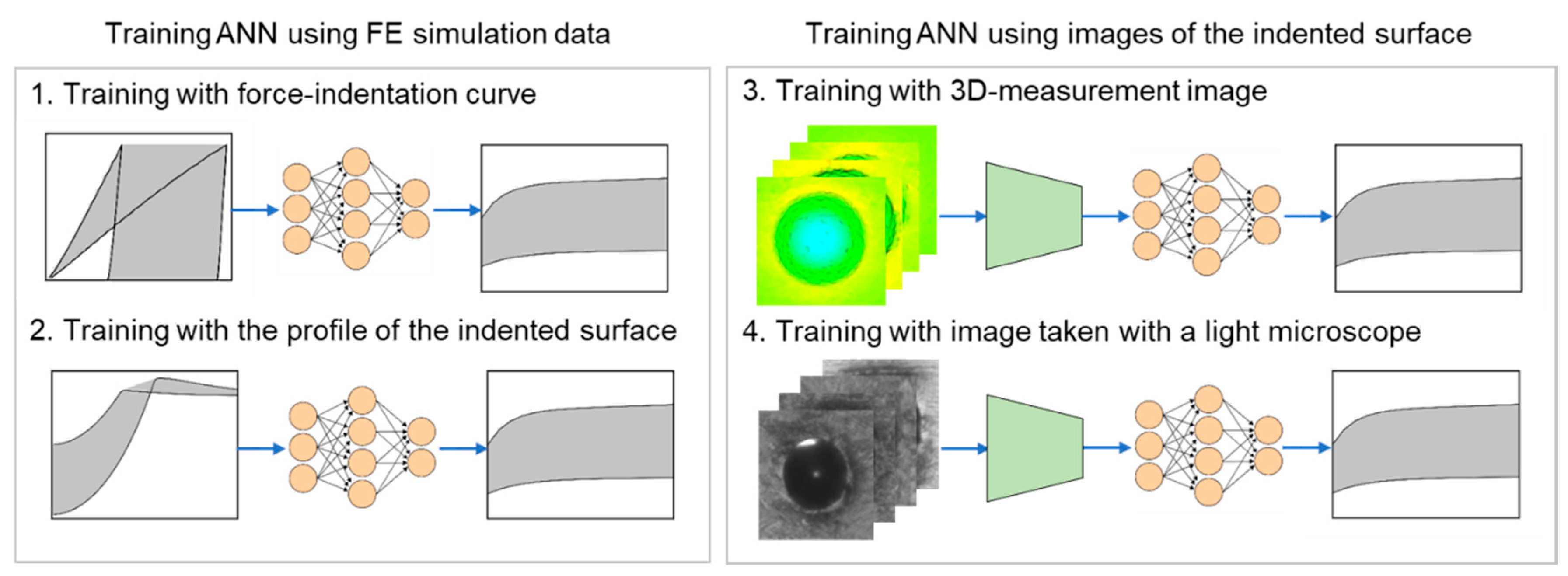
2. Training of the ANN and Application of Computer Vision

As explained in [45], the IIT was performed on the welded, cold rolled, and zinc coated steel plates of DP600 and DP800 with thicknesses of 1 and 1.5 mm, respectively. Moreover, the blank plates of DP1000 with a thickness of 2 mm as well as blank plates of high strength steel S690 with an 8 mm thickness were used. The chemical compositions of used materials are summarized in

Table 1. Chemical compositions of used materials, in weight %.

Material	C	Si	Mn	Cr	Mo	Al	Fe
DP1000	0.11	0.5	2.14	0.03	0.002	0.04	balance
DP800 + ZE	0.14	0.8	1.47	0.1	0.01	0.015	balance
DP600 + ZE75/75	0.1	0.14	1.4	0.16	0.18	0.02	balance
S690QL	0.2	0.8	1.7	1.5	0.7	-	balance

.

The samples were welded with the resistance spot welding (RSW) and laser beam welding (LBW) methods as one of the most common joining technologies in the automobile industry. For the RSW, a C-type servo motor spot weld gun with a frequency of 1000 Hz direct-current transformer (SWAC, Oberhaching, Germany) was used. The LBW was carried out with a Yb:YAG disk laser (Trumpf, Ditzingen, Germany). The beam source of the system had a maximum power of 16 kW and a wavelength of 1030 nm.

Table 2. Welding parameters for the RSW.

Material	Force in kN	Hold Time in ms	Current in kA	Electrode Cape
DP1000	5	140	9	F16
DP600	3.5	260	8	F16

and

Table 3. Welding parameters of the LBW.

Material	Power in kW	Focusing in mm	Speed in m/min
DP1000	2.4	0	1.8
DP600	1.6	0	1.8
S690	8	0	2

summarize the welding parameters used.

2.1. Validation of the Simulation Model of IIT

The validated numerical simulation model of the IIT from [45] was used in this work in order to generate the training datasets in a large quantity (250 datasets). The experimental force–indentation depth curves as well as the profile of the indented surface were compared with the result of the simulation model to validate it. If the difference between two results is in a satisfactory range of accuracy, the FEM (finite element method) model of the IIT, as seen in Figure 2, can be utilized as a validated model to generate the training data.

The penetration tests were carried out with the ZHU2.5 machine (ZwickRoell, Ulm, Germany) and a diamond indenter with a tip radius of 0.2 mm. The maximum penetration depth of this indenter was 60 μm. The maximum load (F) was set to 120 N and the speed of the indenter to 0.05 mm/min.

In order to simulate the indentation test, a two-dimensional numerical simulation was performed by using eight-node axisymmetric elements. A linear–elastic material behavior was selected for the indenter with a Young’s modulus of 1140 GPa and a Poisson’s ratio of 0.07. The geometry and dimensions of the simulation model are shown in Figure 2. A mesh size of 0.0057 mm in the area of the contact between the indenter and specimen and 0.018 mm in the remaining specimen was used.

In this work, the parameters of the Voce nonlinear isotropic hardening material model [46], as shown in Equation (1), were used to describe the behavior of the welded steels as well as the indented samples.

$$\sigma =R_{p0.2}+R_0·{\epsilon }_{pl}+R_{\infty }·(1-e^{\left(-b· {\epsilon }_{pl}\right)})$$

(1)

The parameters R_p0.2 stand for the yield strength, the stress at which the plastic deformation begins. R₀ is the slope of the saturation stress and $R_{\infty }$ stands for the difference between the initial yield strength and saturation stress. The parameter b is a hardening parameter that characterizes the saturation rate and ${\epsilon }_{pl}$ describes the plastic strain. The material model parameters of the base and weld metal from the RSW and LBW techniques are listed in

Table 4. Material model parameter sets for the validation of the ANN [45].

Material		Rp0.2 in MPa	R0 in MPa	R∞ in MPa	b
DP1000	base	630	1100	390	72
	LBW	850	175	437	96
	RSW	906	175	437	96
DP800	base	531	440	422	27
DP600	base	360	710	268	22
	LBW	600	75	420	90
	RSW	867	65	420	110
S690	base	690	393	184	17
	LBW	1000	200	400	100

, according to [45]. These parameters were used to validate the accuracy of the trained ANN.

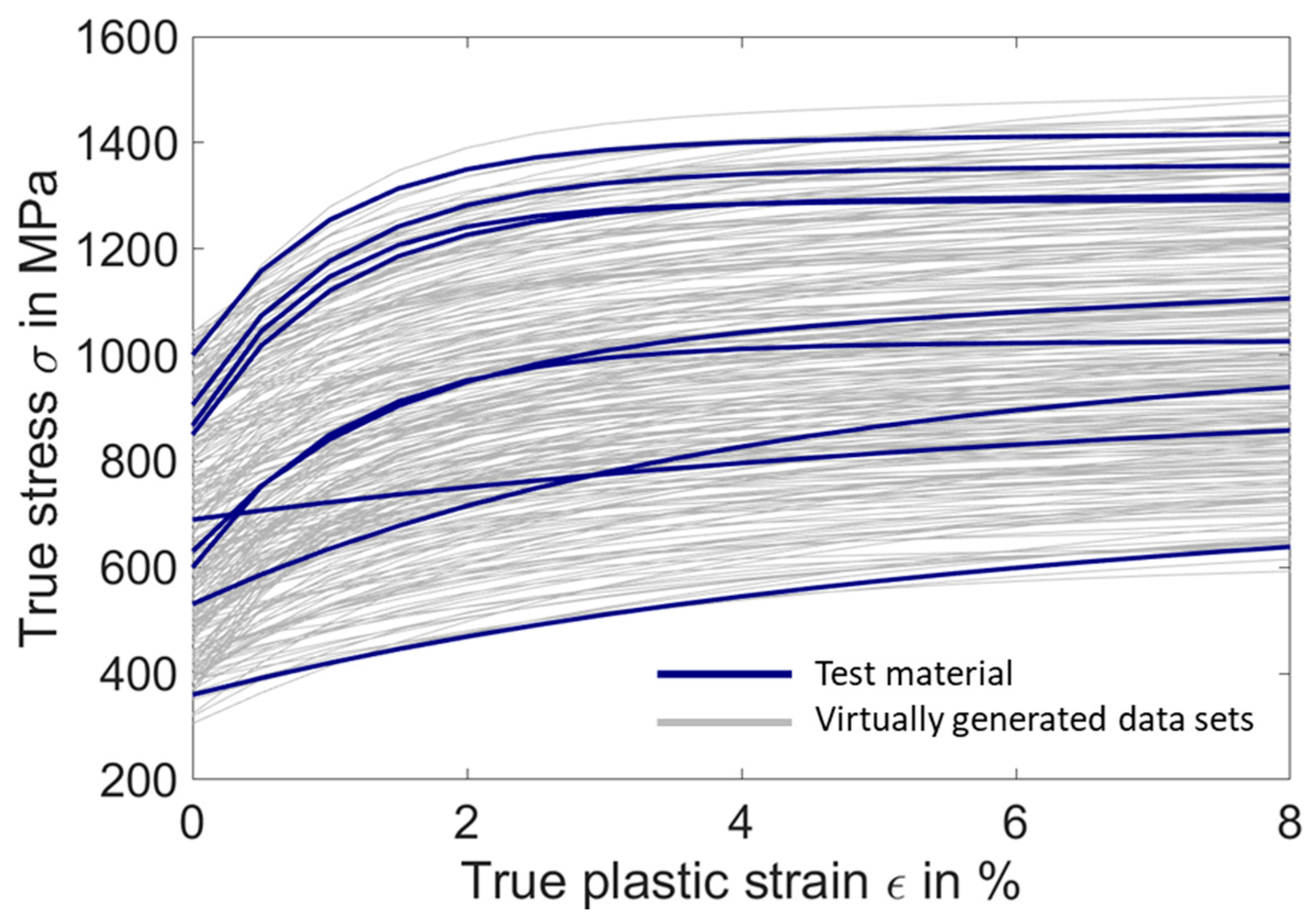
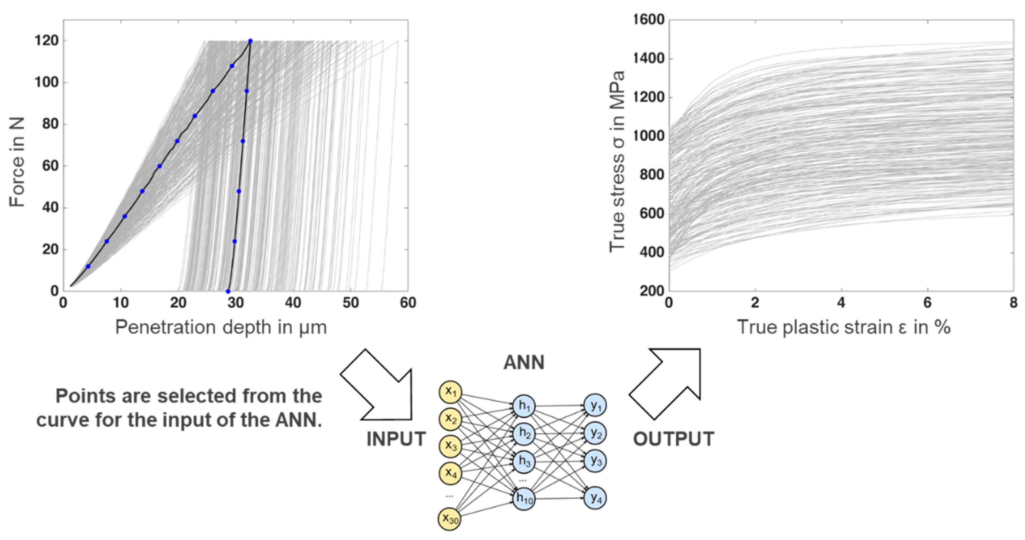
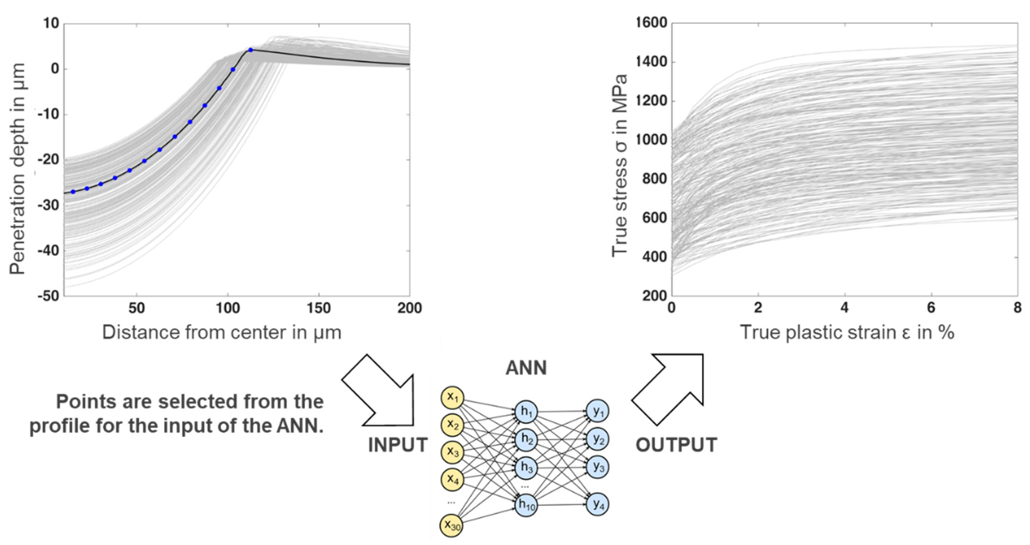
2.2. Generation of Datasets and Training of the ANN

To generate the training data with the validated FEM model, first, a large variety of imaginary material parameter sets (250 parameter sets) were produced within the interval shown in

Table 5. Intervals of material model parameters variation.

Parameter	Interval
Rp0.2 in MPa	[340; 1050]
R0 in MPa	[50; 1150]
R∞ in MPa	[170; 460]
b	[15; 115]

.

For each material model parameter, 250 parameter sets were randomly chosen as the input of the FEM model. In Figure 3, these parameter sets were depicted into 250 imaginary stress–strain curves in gray by inserting the parameters into the Voce nonlinear isotropic hardening model introduced in Equation (1). As seen, the stress–strain curves of the test material (blue) are located between the imaginary curves (gray). However, they have to be excluded, since they must stay unknown to the ANN. Moreover, the stress–strain diagrams of these imaginary materials were stored as the outputs for the training of the ANN, as shown in Figure 4 and Figure 5.

Both corresponding force–indentation depth curves and the indented surface profiles were numerically calculated. The selected data points of these curves, as shown in Figure 4 and Figure 5, were stored as the inputs to train the ANN. With this step, the 250 training datasets that consisted of input and output for the ANN were created.

In the training phase, 15 data points on every curve were chosen as an input for the training of the ANN. As seen in Figure 4, the data points were distributed throughout the loading and unloading parts. The tenth data point was set as at the end of the loading phase at the maximum force level. The complete force release is represented by the fifteenth data point.

Similarly, as seen in Figure 5, in order to obtain the same dimensions of vectors for ANN training, 15 data points between the lowest and highest point of the indented surface were considered. Each selected data point has two lots of information, which leads to a total of 30 values as the input of the training datasets.

In addition, the input and the output of the training data were normalized with linear scale transformation to increase the performance of the ANN and speed up the calculation [47]. The input layer of the ANN comprises 30 neurons, the hidden layer 10 neurons, and the output layer has four neurons for the four material model parameters represented in Table 5. In order to avoid overfitting during the supervised training, an early stopping method was implemented [48]. In this technique, the training datasets were divided into three subsets such as training, validation, and testing, which evaluated the generalization of the ANN toward unknown data. The division of the dataset into three subsets was performed randomly with the allocation ratio of 8:1:1 to the training (80%), testing (10%), and validation (10%) data, respectively. The tan-Sigmoid (Tansig) and linear (Purelin) transfer function were used as the activation function in the hidden and output layer. The learning rate of the network was 0.01. The backpropagation with the Levenberg–Marquardt optimization algorithm [49] was implemented for updating the weights and biases of the ANN.

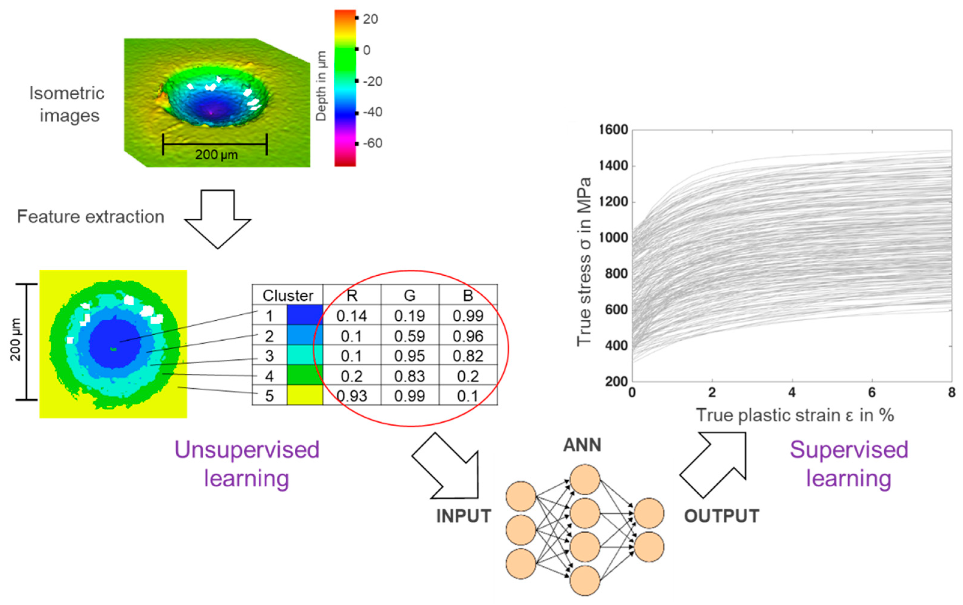
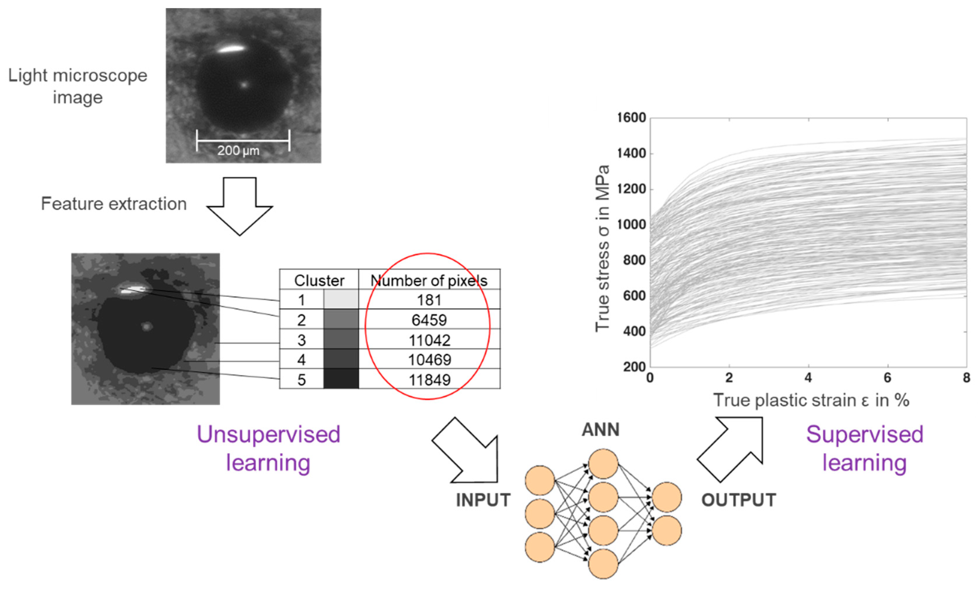
2.3. Processing the Indented Surface Images and Training of the ANN

The surface of the indented specimens was visually analyzed by using the Alicona infinite focus as a contactless 3D surface measurement system [50]. The information related to the deformation of the indented surface in each point was recorded in 2D and 3D. First, the images were processed to bring them into the same color scale as a measurement reference as well as the same size, brightness, and pixel. In total, nine images from the surface of the specimens mentioned in Table 4 were captured and processed. Each final image had a square shape with the same brightness and contained 170 × 170 pixels. The pixels had color values based on a RGB format. The input data needed to be dimensionally reduced to have less complexity before employing them as the input to train the ANN. By performing k-means clustering, the RGB values in each pixel of the image were observed and partitioned into five optimal clusters, which were extracted by analyzing the Silhouette index of each data point in each cluster of the k-mean results. The algorithm returned the centroid of the clusters based on the RGB values and additionally assigned every pixel to its proper group. This transformation is depicted in Figure 6 in the unsupervised training part.

The clustered colors were then sorted according to the hue-saturation value [51], which was used to represent the depth from the 3D-measurement. By sorting the colors, it was guaranteed that the first centroid showed the region with the deepest indentation, located mostly in the middle of the image. The last centroid defined the highest region of the surface unaffected by the indentation or pile-up. Finally, the RGB values of each centroid were used as input for the training dataset. With this, the image that originally had 170 × 170 × 3 variables was reduced to a total of 5 × 3 parameters. Then, these parameters, shown in the red circle in Figure 6, were packed into a vector (1 × 15) and this vector was used as input data. The material parameters of each image were used as the corresponding output. In the end, 15 input, seven hidden, and four output neurons were needed to train the ANN with images from the 3D-measurement. This procedure is shown in Figure 6.

Furthermore, the indented surface was examined under a simple light microscope (Zeiss, Jena, Germany) with 40× magnification. All images were captured under the same conditions such as lightning and camera position. In total, 11 grayscale images were successfully captured with the light microscope from the materials mentioned in Table 4 and the corresponding heat affected zones. The images had a square shape with dimensions of 200 × 200 pixels. Image segmentation with k-means clustering was also performed on them. The optimal number of clusters, extracted by analyzing the Silhouette index of each data point in each cluster of k-mean results, was 5. Since the images were in grayscale, the centroids of the clusters had three identical RGB values. This parameter represents the brightness, with 0 defined as black and 1 as white. The indented area is recognizable with its darker color as well as its surrounding. The size of the indented area is different between images and depends on the depth of the penetration. Therefore, instead of the color values of each centroid, the number of pixels assigned to each cluster was considered as the input of the training dataset. The centroids of five clusters were then sorted from light to dark. In this step, the ANN was constructed with five inputs, five hidden, and four output neurons for the training with images from the light microscope. The tan-Sigmoid (Tansig) and linear (Purelin) transfer function were used as the activation function in the hidden and output layer. The learning rate of the network was 0.01. The procedure is described in Figure 7.

Due to the limited training dataset, backpropagation, together with the Levenberg–Marquadt optimization and Bayesian regularization was used to construct the ANN. By using the Bayesian criterion for stopping the training, the algorithm does not need a further validation subset [52]. This algorithm needs more computation time, but is suitable for training with limited data.

Moreover, the performance of the ANN was analyzed with the cross validation method. Each image set taken from the 3D-measurement and the light microscope were trained three times. In each training, two of them were randomly excluded from the training and used as test data to check the accuracy of the trained ANN.

3. Results and Discussions

The trained ANN must be tested and validated to evaluate its performance and accuracy. The data used for the testing was not a part of the training dataset and therefore was unknown to the ANN. By using the unknown data in the test phase, the precision, generalization, and flexibility of the ANN were investigated.

The validated simulation model of the IIT from [45] was used to generate datasets to train the ANN. The results showed very good agreement between the simulated force–indentation depth curves as well as the profiles of the indented surface and the measurement, more specifically in the heat affected zone and weld nugget.

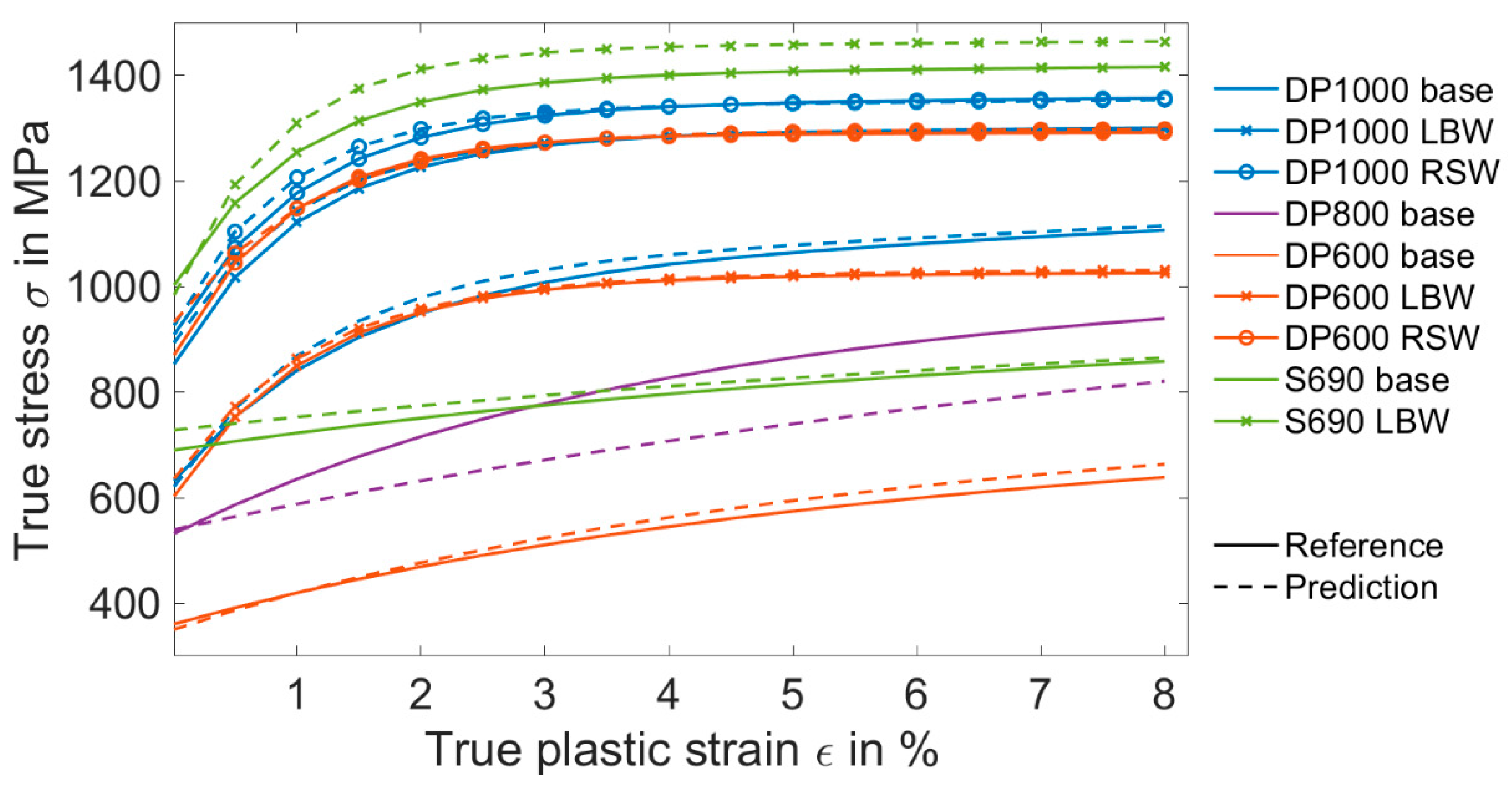
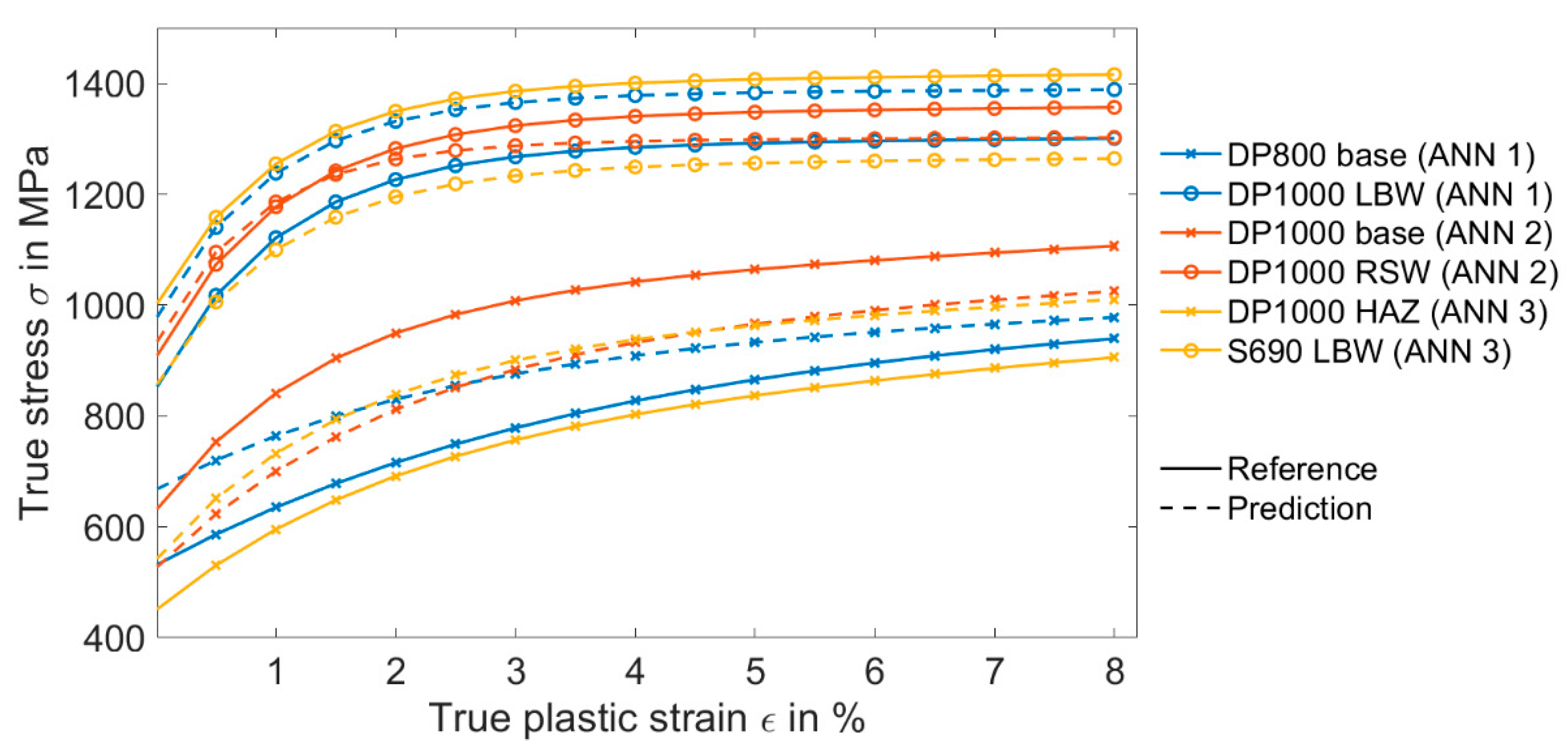
3.1. Validation of the ANN Trained with Simulation Data

The evaluation of the regression value is known as a common method to check the accuracy and flexibility of the trained ANN. This is possible by comparing the predicted values by the ANN and the desired outputs in a regression plot. The regression coefficient is the slope of the best fit line between the predicted values and desired outputs.

Table 6. Regression coefficients obtained by comparing the desired outputs and outputs of the trained ANN.

Data set	Regression Coefficient
	Rp0.2	R0	R∞	b
Force-indentation depth curve	0.98	0.9	0.81	0.73
Profile of indented surface	0.99	0.99	0.98	0.95

shows the resulting regression coefficients of the ANN trained with the data of force–indentation curves and the surface deformations obtained from the simulation data.

The regression coefficient of yield strength R_p0.2 was bigger than the other parameters and indicates that the ANN can approximate yield strength with higher accuracy. Using the information related to the surface deformation as the training dataset leads to more precise results compared with the force–indentation depth data. Nevertheless, the regression value is only one criterion in which to control how well the ANN adjusts its weight and biases toward the training data. A detailed evaluation on the accuracy of the ANN must be performed through its evaluation with the unknown data.

As seen in Figure 8, there was a very good correlation between the predicted material model parameters and the reference data. The ANN can predict the yield strength R_p0.2 more accurately than the three other parameters. The mean absolute percentage error (MAPE) between the reference and prediction of R_p0.2 and R_∞ were 7% and 18%, respectively, for the whole test data. Other material model parameters, R₀ and b, can be predicted with the MAPE of 50%. The larger MAPE value of these parameters explains the reason of deviation in the strain hardening part of the stress–strain curve. However, this high value of MAPE does not have a considerable effect on the stress–strain curve. The sensitivity analysis revealed that R_p0.2 is the most important parameter of the chosen material model. The effect of the strain hardening material parameters was minimal, particularly R₀ and b. Therefore, the high value of the prediction error did not lead to the considerable differences in the stress–strain curve.

Additionally, the trained ANN with the information of the indented surface profiles showed good performance in terms of generalization, as seen in Figure 9. The better regression values, according to Table 6, indicate that the ANN can predict the material model parameters more precisely. The yield strength R_p0.2 was again the most accurate parameter with a MAPE value of 4%. The Voce nonlinear isotropic hardening material model parameters were also determined, with the MAPE value of less than 21%.

These positive results imply that an ANN trained with the profiles of the indented surface predict the material parameters with a higher accuracy. This may be caused by the strong dependency between the indented surface and the hardening plastic behavior.

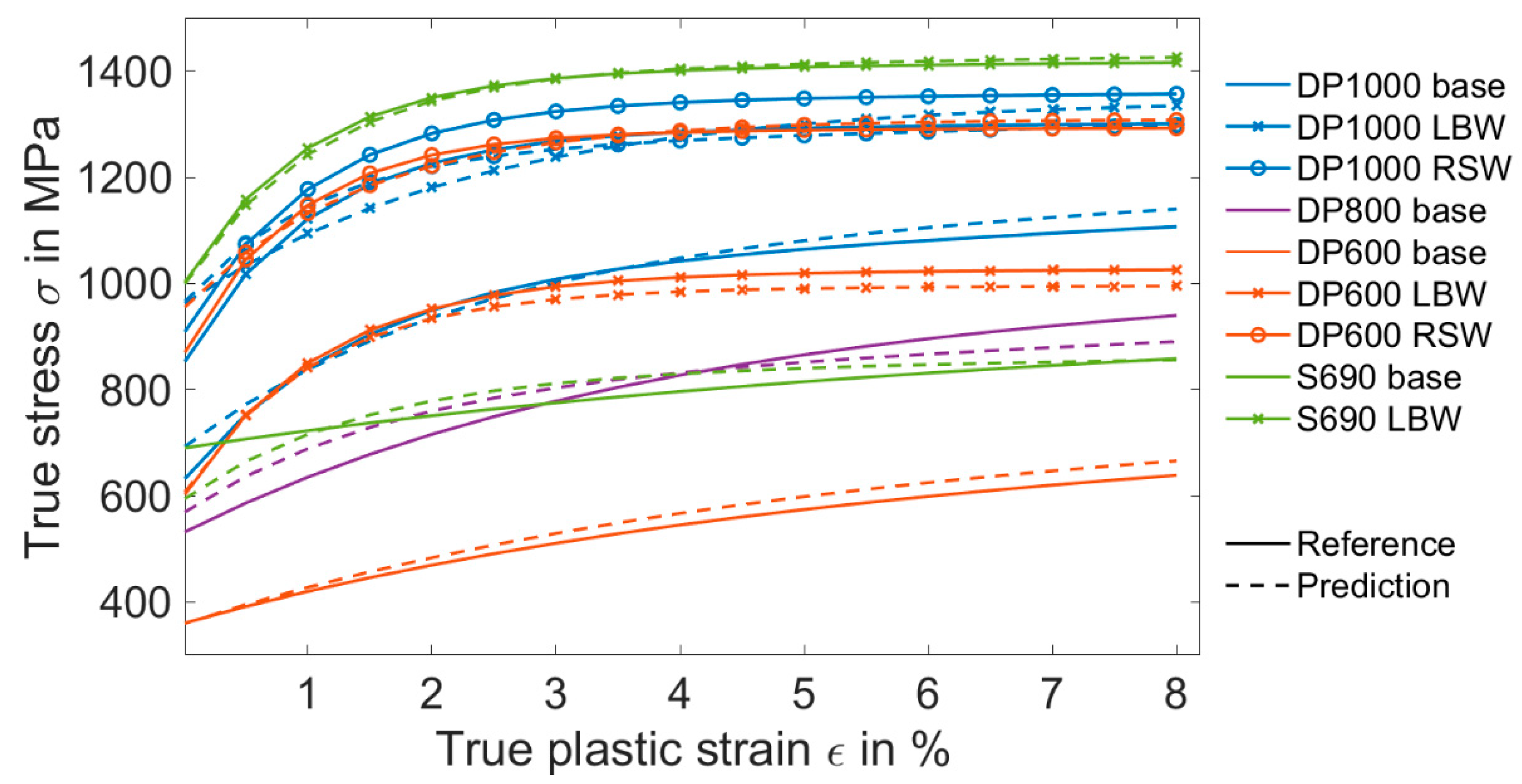
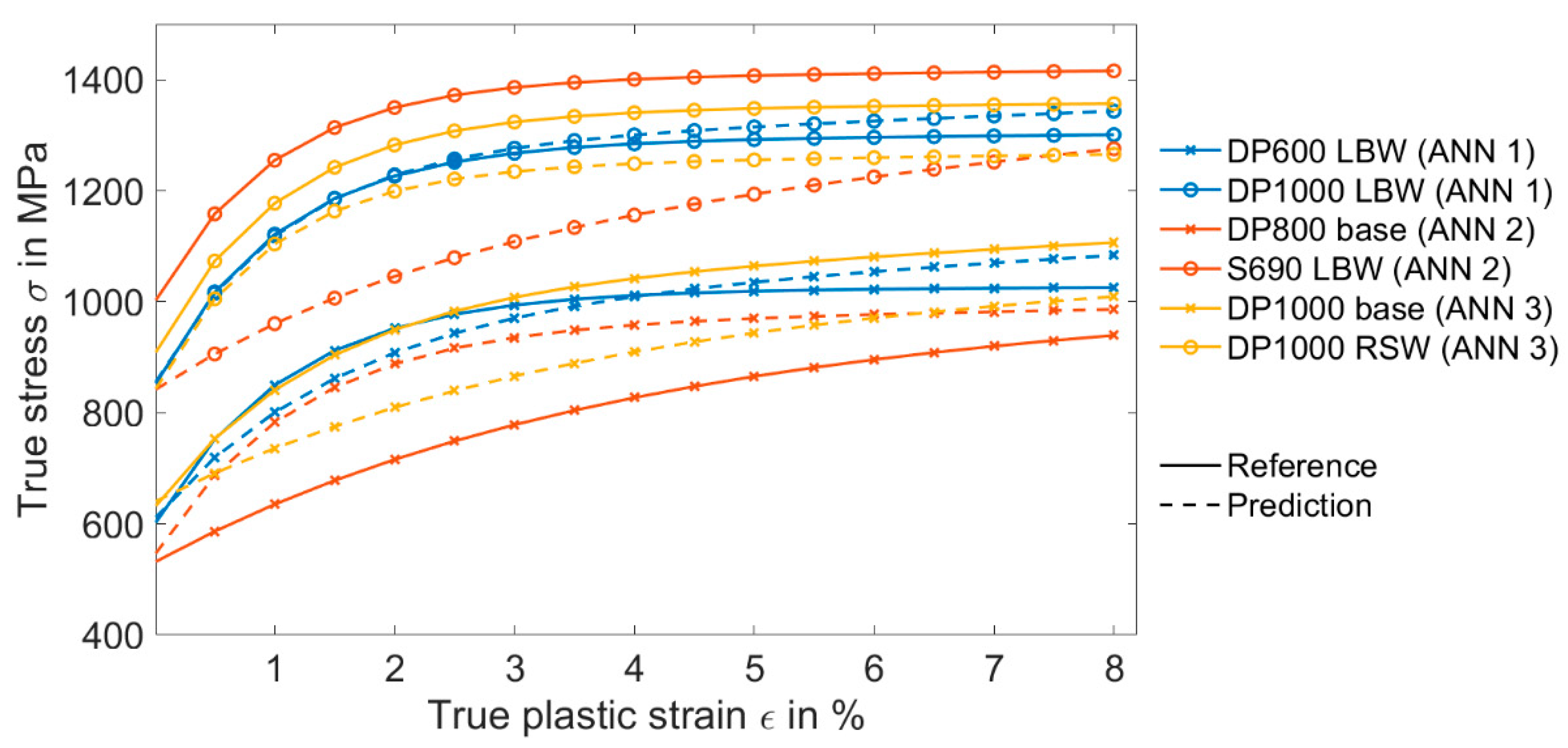
3.2. Validation of the ANN Trained with the Images of the Deformed Surface

First, the Mann–Whitney–Wilcoxon test [53] was conducted on the representative clusters of each image. The test with the resulting p-value of less than 0.5 showed that each cluster was unique and independent of the others. In the next step, in order to evaluate the accuracy of the trained ANN with images of 3D-measurement, the predicted values were compared with the reference values from Table 4. As seen in Figure 10, the ANN could determine the stress–strain curves with a lower accuracy in comparison with the previous section. The prediction MAPE of yield strength R_p0.2 varied between 3% to 26%. Due to the importance of R_p0.2 in the chosen material model, a small variation of this parameter can significantly change the resulting stress–strain curve. This higher value of MAPE was mainly due to the limited number of the training dataset.

Figure 11 shows the comparison between the predicted material model parameters from the ANN trained with the grayscale images taken with a simple light microscope and the reference values from Table 4. It seems that the ANN had difficulties in determining the strain hardening parameters such as R₀ and b. However, it could predict R_p0.2 and R_∞ with a MAPE value less than 16% and 25%, respectively.

As seen in Figure 9 and Figure 10, the ANN trained with the data extracted from images could predict the material behavior. It is expected that by increasing the number in the training dataset, which was less than 10 images in this case, the ANN could predict the material parameters with higher precision. Once again, to obtain the ANN with high accuracy performed in Section 3.1, 250 datasets were used to train the ANN with the force–indentation depth curves and profile of the deformed surface.

Four independent methods were introduced to characterize the mechanical properties of the welded steels locally, in the attempt to make the procedure of material characterization less complicated for the user. The last approach (light microscope image) can be undertaken with only a simple light microscope.

4. Summary and Conclusions

It was shown that it is possible to determine the mechanical properties of welded high strength steels with four completely independent approaches: (1) force–indentation curve, (2) profile of the indented surface, (3) 3D-measurement image captured from the surface of the indented specimen, and (4) image taken from the indented surface with a simple light microscope. Moreover, it is necessary to mention that only the first approach needs an instrumented indentation machine. The other three methods can be performed by only pushing a simple indenter into the surface of a specimen without using the instrumented indentation machine.

The presented results show that the ANN trained with data of deformed surface profiles or force–indentation curves can predict the material behavior of the welded high strength steels with a very high accuracy. It was observed that this method is strongly robust for the determination of the yield strength. However, it is also possible to calculate the other material model parameters with satisfactory precision.

Furthermore, it was shown that the images taken from the surface of an indented specimen can be analyzed with computer vision algorithms to find a correlation between them and the mechanical properties of materials. Nevertheless, the accuracy and flexibility of this method can be improved by increasing the number in the training dataset.

References

1. Den Uijl, N.; Moolevliet, T.; Mennes, A.; van der Ellen, A.A.; Smith, S.; van der Veldt, T.; Okada, T.; Nishibata, H.; Uchihara, M.; Fukui, K. Performance of resistance spot-welded joints in advanced high-strength steel in static and dynamic tensile tests. Weld. World 2012, 56, 51–63. [Google Scholar] [CrossRef]
2. Brauser, S. Phasenumwandlung und Lokale Mechanische Eigenschaften von TRIP Stahl Beim Simulierten und Realen Widerstandspunktschweißprozess; BAM-Dissertationsreihe: Berlin, Germany, 2013; Volume 100. [Google Scholar]
3. Oliver, W.C.; Pharr, G.M. Measurement of hardness and elastic modulus by instrumented indentation: Advances in understanding and refinemeants to methodology. J. Mater. Res. 2004, 19, 3–20. [Google Scholar] [CrossRef]
4. Chung, K.-H.; Lee, W.; Kim, J.H.; Kim, C.; Park, S.H.; Kwon, D.; Chung, K. Characterization of mechanical properties by indentation tests and FE analysis—Validation by application to a weld zone of DP590 steel. Int. J. Solids Struct. 2009, 46, 344–363. [Google Scholar] [CrossRef] [Green Version]
5. Huber, N. Anwendung Neuronaler Netze bei nichtlinearen Problemen der Mechanik. Habilitation; Universität Karlsruhe: Karlsruhe, Germany, 2000. [Google Scholar]
6. ISO. ISO/TR 29381. Metallic Materials—Measurement of Mechanical Properties by an Instrumented Indentation Test—Indentation Tensile Properties; ISO: Genève, Switzerland, 2009. [Google Scholar]
7. Haušild, P.; Materna, A.; Nohava, J. On the identification of stress–strain relation by instrumented indentation with spherical indenter. Mater. Des. 2012, 37, 373–378. [Google Scholar] [CrossRef]
8. Moussa, C.; Bartier, O.; Mauvoisin, G.; Pilvin, P.; Delattre, G. Characterization of homogenous and plastically graded materials with spherical indentation and inverse analysis. J. Mater. Res. 2012, 27, 20–27. [Google Scholar] [CrossRef] [Green Version]
9. Habbab, H.; Mellor, B.; Syngellakis, S. Post-yield characterisation of metals with significant pile-up through spherical indentations. Acta Mater. 2006, 54, 1965–1973. [Google Scholar] [CrossRef] [Green Version]
10. Ahn, J.-H.; Kwon, D. Derivation of plastic stress-strain relationship from ball indentations: Examination of strain definition and pileup effect. J. Mater. Res. 2001, 16, 3170–3178. [Google Scholar] [CrossRef]
11. Jeon, E.-C.; Park, J.-S.; Kwon, D. Statistical analysis of experimental parameters in continuous indentation tests using Taguchi method. J. Eng. Mater. Technol. 2003, 125, 406–411. [Google Scholar] [CrossRef]
12. Karthik, V.; Visweswaran, P.; Bhushan, A.; Pawaskar, D.; Kasiviswanathan, K.; Jayakumar, T.; Raj, B. Finite element analysis of spherical indentation to study pile-up/sink-in phenomena in steels and experimental validation. Int. J. Mech. Sci. 2012, 54, 74–83. [Google Scholar] [CrossRef]
13. Bouzakis, K.; Michailidis, N.; Erkens, G. Thin hard coating stress-strain curve determination through a FEM supported evaluation of nano-indentation test results. Surf. Coat. Technol. 2001, 142, 102–109. [Google Scholar] [CrossRef]
14. Dao, M.; Chollacoop, N.; Van Vliet, K.; Venkatesh, T.; Suresh, S. Computational modeling of the forward and reverse problems in instrumented sharp indentation. Acta Mater. 2001, 49, 3899–3918. [Google Scholar] [CrossRef] [Green Version]
15. Bucaille, J.; Stauss, S.; Felder, E.; Michler, J. Determination of plastic properties of metals by instrumented indentation using different sharp indenters. Acta Mater. 2003, 51, 1663–1678. [Google Scholar] [CrossRef]
16. Spary, I.; Bushby, A.; Jennett, N. On indentation size effect in spherical indentation. Philos. Mag. 2006, 86, 5581–5593. [Google Scholar] [CrossRef] [Green Version]
17. Bouzakis, K.; Michailidis, N. Indenter surface area and hardness determination by means of a FEM-supported simulation of nano-indentation. Thin Solid Films 2006, 494, 155–160. [Google Scholar] [CrossRef]
18. Huber, N.; Konstantinidis, A.; Tsakmakis, C. Determination of poisson’s ratio by spherical indentation using neural networks—part I: Theory. J. Mech. Phys. Solids 2001, 68, 218–223. [Google Scholar] [CrossRef]
19. Huber, N.; Tsakmakis, C. Determination of poisson’s ratio by spherical indentation using neural networks—part II: Identification method. J. Appl. Mech. 2001, 68, 224. [Google Scholar] [CrossRef]
20. Tyulyukovskiy, E.; Huber, N. Identification of viscoplastic material parameters from spherical indentation data: Part I. neural networks. J. Mater. Res. 2006, 21, 664–676. [Google Scholar] [CrossRef]
21. Klötzer, D.; Ullner, C.; Tyulyukovskiy, E.; Huber, N. Identification of viscoplastic material parameters from spherical indentation data: Part II. experimental validation of the method. J. Mater. Res. 2006, 21, 677–684. [Google Scholar] [CrossRef]
22. Huber, N.; Tsakmakis, C. Determination of constitutive properties fromspherical indentation data using neural networks. part I: The case of pure kinematic hardening in plasticity laws. J. Mech. Phys. Solids 1999, 47, 1569–1588. [Google Scholar] [CrossRef]
23. Huber, N.; Tsakmakis, C. Determination of constitutive properties fromspherical indentation data using neural networks. part II: Plasticity with nonlinear isotropic and kinematichardening. J. Mech. Phys. Solids 1999, 47, 1589–1607. [Google Scholar] [CrossRef]
24. Ullner, C.; Brauser, S.; Subaric-Leitis, A.; Weber, G.; Rethmeier, M. Determination of local stress–strain properties of resistance spot-welded joints of advanced high-strength steels using the instrumented indentation test. J. Mater. Sci. 2012, 47, 1504–1513. [Google Scholar] [CrossRef]
25. Rao, D.; Heerens, J.; Alves Pinheiro, G.; dos Santos, J.; Huber, N. On characterisation of local stress–strain properties in friction stir welded aluminium AA 5083 sheets using micro-tensile specimen testing and instrumented indentation technique. Mater. Sci. Eng. A 2010, 527, 5018–5025. [Google Scholar] [CrossRef] [Green Version]
26. Yagawa, G.; Okuda, H. Neural networks in computational mechanics. Arch. Comput. Methods Eng. 1996, 3, 435. [Google Scholar] [CrossRef]
27. Li, X.; Liu, Z.; Cui, S.; Luo, C.; Li, C.; Zhuang, Z. Predicting the effective mechanical property of heterogeneous materials by image based modelling and deep learning. Comput. Methods Appl. Mech. Eng. 2019, 347, 735–753. [Google Scholar] [CrossRef] [Green Version]
28. Ye, S.; Li, B.; Li, Q.; Zhao, H.; Feng, X. Deep neural network method for predicting the mechanical properties of composites. Appl. Phys. Lett. 2019, 115, 161901. [Google Scholar] [CrossRef]
29. Xu, Z.; Liu, X.; Zhang, K. Mechanical properties prediction for hot rolled alloy steel using convolutional neural network. IEEE Access 2019, 7, 2169–3536. [Google Scholar] [CrossRef]
30. Chun, P.-J.; Yamane, T.; Izumi, S.; Kameda, T. Evaluation of tensile performance of steel members by analysis of corroded steel surface using deep learning. Metals 2019, 9, 1259. [Google Scholar] [CrossRef] [Green Version]
31. Psuj, G. Multi-Sensor Data Integration Using Deep learning for characterization of defects in steel elements. Sensors 2018, 18, 292. [Google Scholar] [CrossRef] [Green Version]
32. Michie, D. “Memo” Functions and machine learning. Nature 1968, 218, 19–22. [Google Scholar] [CrossRef]
33. Sathya, R.; Abraham, A. Comparison of supervised and unsupervised learning algorithms for pattern classification. J. Adv. Res. Artif. Intell. 2013, 2, 34–38. [Google Scholar] [CrossRef] [Green Version]
34. Basheer, I.; Hajmeer, M. Artificial neural networks: Fundamentals, computing, design, and application. J. Microbiol. Methods 2000, 43, 3–31. [Google Scholar] [CrossRef]
35. Shafi, I.; Ahmad, J.; Shah, S.I.; Kashif, F.M. Impact of Varying Neurons and Hidden Layers in Neural Network Architecture for a Time Frequency Application. In Proceedings of the IEEE International Multitopic Conference, Islāmābād, Pakistan, 23–24 December 2006. [Google Scholar]
36. Zheng, H.; Fang, L.; Ji, M.; Strese, M.; Ozer, Y.; Steinbach, E. Deep learning for surface material classification using haptic and visual information. IEEE Trans. Multimed. 2016, 18, 2407–2416. [Google Scholar] [CrossRef]
37. Azimi, S.; Britz, D.; Engstler, M.; Fritz, M.; Mücklich, F. Advanced steel microstructural classification by deep learning methods. Sci. Rep. 2018, 8, 2128. [Google Scholar] [CrossRef] [PubMed]
38. Soukup, D.; Huber-Mörk, R. Convolutional neural networks for steel surface defect detection from photometric stereo images. Adv. Vis. Comput. 2014, 8887, 668–677. [Google Scholar]
39. Maitra, D.S.; Bhattacharya, U.; Parui, S.K. CNN based common approach to handwritten character recognition of multiple scripts. In Proceedings of the 13th International Conference on Document Analysis and Recognition (ICDAR), Nancy, France, 23–26 August 2015. [Google Scholar]
40. Shapiro, L.G.; Stockman, G.C. Computer Vision; Prentice Hall: Upper Saddle River, NJ, USA, 2001. [Google Scholar]
41. Javaheri, A.; Moghadamneja, N.; Keshavarz, H.; Javaheri, E.; Dobbins, C.; Momeni, E.; Rawassizadeh, R. Public vs. Media Opinion on Robots and Their Evolution over Recent Years. arXiv 2019, arXiv:1905.01615. [Google Scholar]
42. Rawassizadeh, R.; Dobbins, C.; Akbari, M.; Pazzani, M. Indexing multivariate mobile data through spatio-temporal event detection and clustering. Sensors 2019, 19, 448. [Google Scholar] [CrossRef] [Green Version]
43. Dobbins, C.; Rawassizadeh, R. Clustering of Physical Activities for Quantified Self and mHealth Applications. In Proceedings of the IEEE International Conference on Computer and Information Technology, Liverpool, UK, 26–28 October 2015; pp. 1423–1428. [Google Scholar]
44. Javaheri, E.; Pittner, A.; Graf, B.; Rethmeier, M. Mechanical properties characterization of resistance spot welded DP1000 steel under uniaxial tensile test. Materialprufung 2019, 61, 527–532. [Google Scholar] [CrossRef]
45. Javaheri, E.; Lubritz, J.; Graf, B.; Rethmeier, M. Mechanical properties characterization of welded automotive steels. Metals 2020, 10, 1. [Google Scholar] [CrossRef] [Green Version]
46. Lemaitre, J.; Chaboche, J.L. Mechanics of Solid Materials; Cambridge University Press: Cambridge, UK, 1990. [Google Scholar]
47. Sola, J.; Sevilla, J. Importance of input data normalization for the application of neural networks to complex industrial problems. IEEE Trans. Nuclear Sci. 1997, 44, 1464–1468. [Google Scholar] [CrossRef]
48. Prechelt, L. Automatic early stopping using cross validation: Quantifying the criteria. Neural Netw. 1998, 11, 761–767. [Google Scholar] [CrossRef] [Green Version]
49. Hagan, M.T.; Menhaj, M.B. Training feedforward networks with the Marquardt algorithm. IEEE Trans. Neural Netw. 1994, 5, 989–993. [Google Scholar] [CrossRef]
50. Danzl, R.; Helmli, F.; Scherer, S. Focus Variation—A New Technology for High Resolution Optical 3D Surface Metrology. In Proceedings of the 10th International Conference of the Slovenian Society for Non-Destructive Testing, Ljubljana, Slovenia, 1–3 September 2009; pp. 484–491. [Google Scholar]
51. Cheng, H.D.; Jiang, X.H.; Sun, Y.; Wang, J. Color image segmentation: Advances and prospects. Pattern Recognit. 2001, 34, 2259–2281. [Google Scholar] [CrossRef]
52. Burden, F.; Winkler, D. Bayesian Regularization of Neural Networks. In Artificial Neural Networks: Methods and Applications; Humana Press: Totowa, NJ, USA, 2008; pp. 23–42. [Google Scholar]
53. Mann, H.B.; Whitney, D.R. On a test of whether one of two random variables is stochastically larger than the other. Ann. Math. Statist. 1947, 18, 50–60. [Google Scholar] [CrossRef]
Figure 1. General workflow of the ANN training with the four different types of database.
Metals 10 00163 g001
Figure 2. Geometry of the simulation model of IIT.
Metals 10 00163 g002
Figure 3. Stress–strain curves from the variation of the material model parameters.
Metals 10 00163 g003
Figure 4. Force–indentation depth curves generated by the FEM model and the corresponding stress–strain diagrams as the training datasets of the ANN.
Metals 10 00163 g004
Figure 5. Indented surface profiles generated by the FEM model and the corresponding stress-strain curves as the training datasets of the ANN.
Metals 10 00163 g005
Figure 6. Feature extraction of the images from the 3D measurements and training of the ANN.
Metals 10 00163 g006
Figure 7. Feature extraction of the light microscope images and training of the ANN.
Metals 10 00163 g007
Figure 8. Comparison between the output of the ANN trained with the force–indentation curves and the reference values from Table 4.
Metals 10 00163 g008
Figure 9. Comparison between the output of the ANN trained with the data of the indented surface profiles and the reference values from Table 4.
Metals 10 00163 g009
Figure 10. Comparison between the output of the ANN and the reference values from Table 4, where the ANN trained with the features extracted from images shows the deformation of the indented surface (3D-measurement image).
Metals 10 00163 g010
Figure 11. Comparison between the output of the ANN and the reference values from Table 4, where the ANN was trained with the features extracted from images taken with a light microscope from the indented surface.
Metals 10 00163 g011