On the Influence of Control Type and Strain Rate on the Lifetime of 50CrMo4

 ,
,  ,
,  ,
,  ,
,
Abstract

1. Introduction
2. Effects of Strain Rate on Deformation and Fatigue
2.1. Intrinsic Effects
2.2. Extrinsic Effects
3. Experimental Foundation
4. Method
4.1. Correction for Control Type
4.2. Statistical Analysis
5. Results
6. Analysis
7. Summary
8. Outlook
Author Contributions
Funding
Acknowledgments
Conflicts of Interest
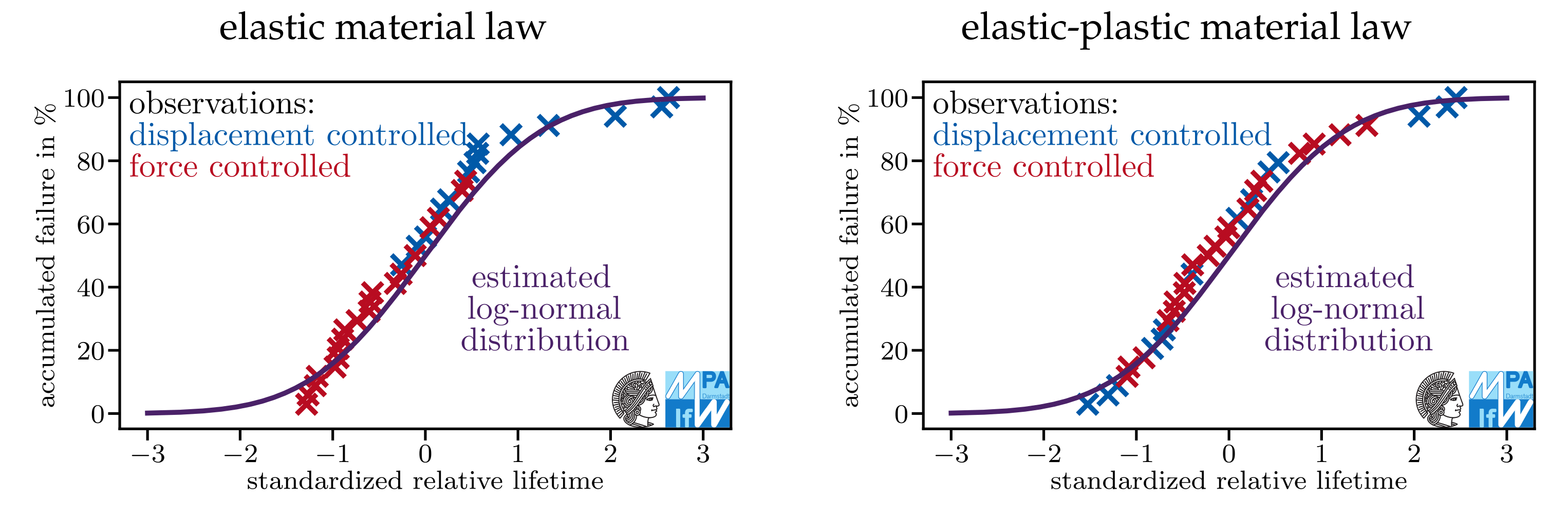
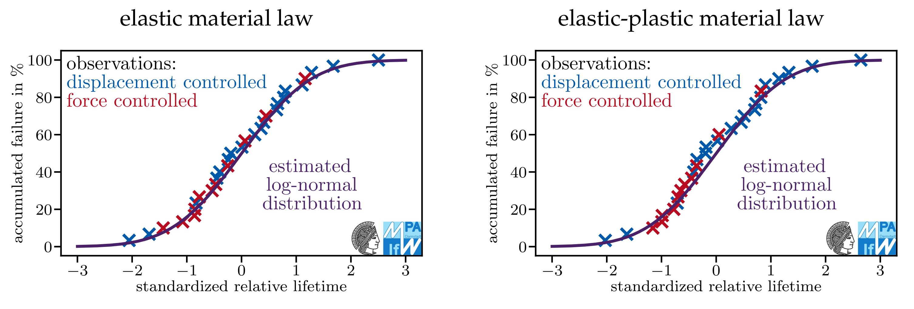
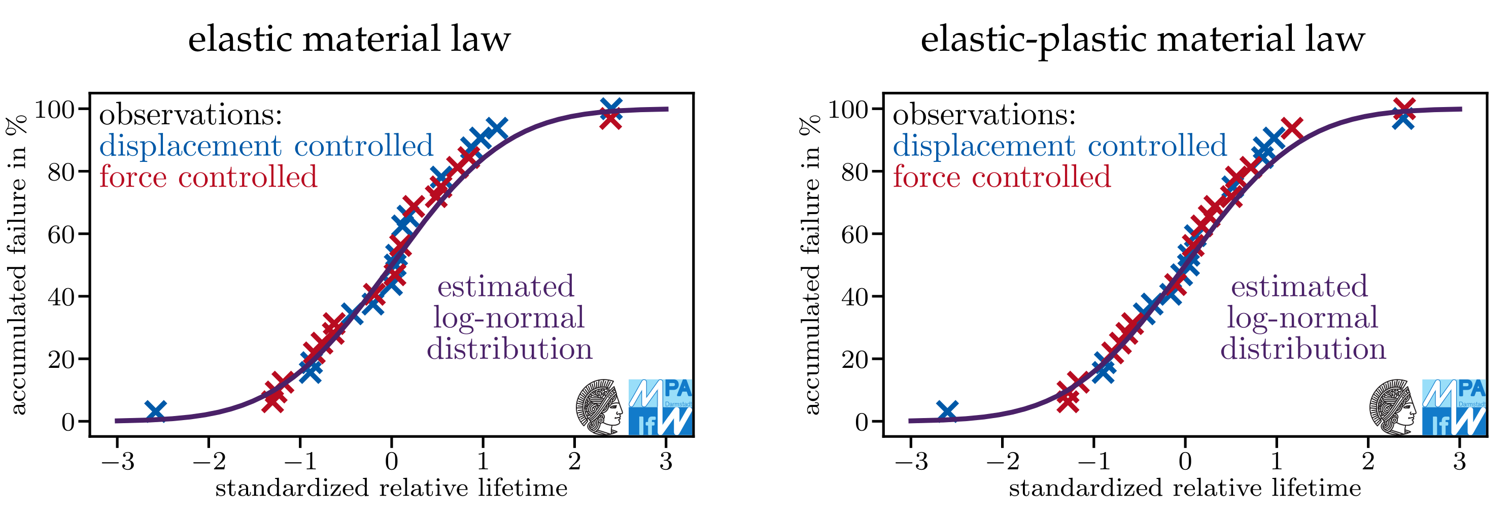
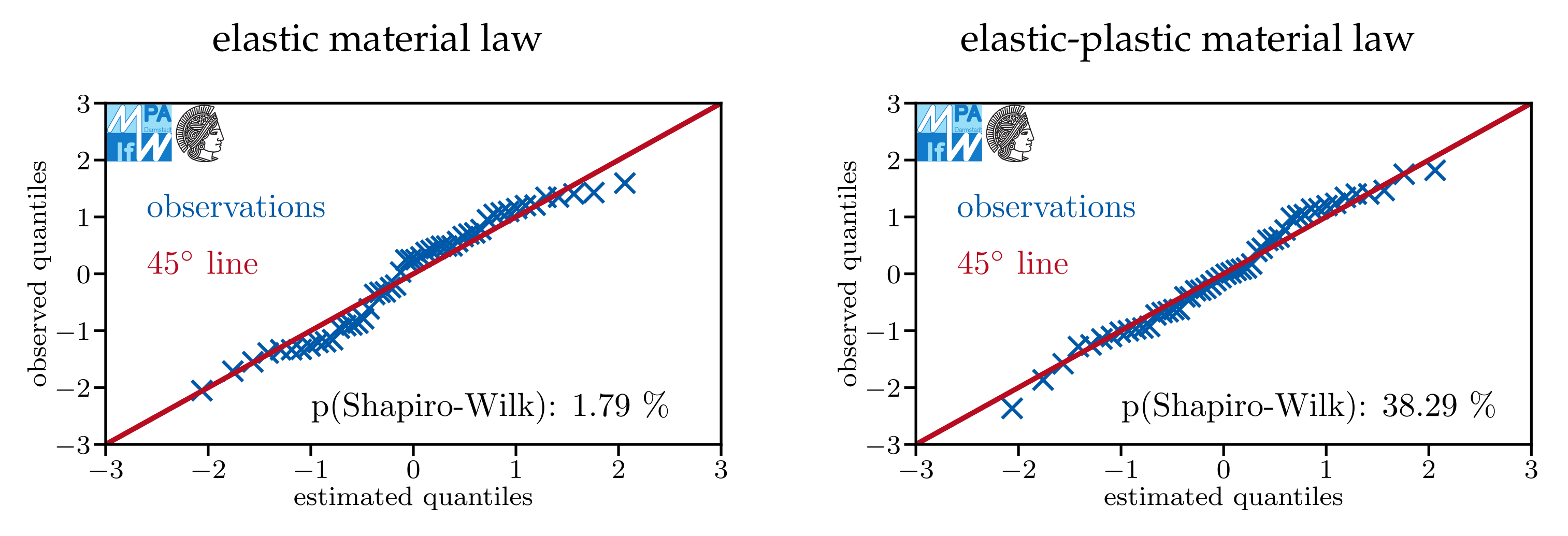
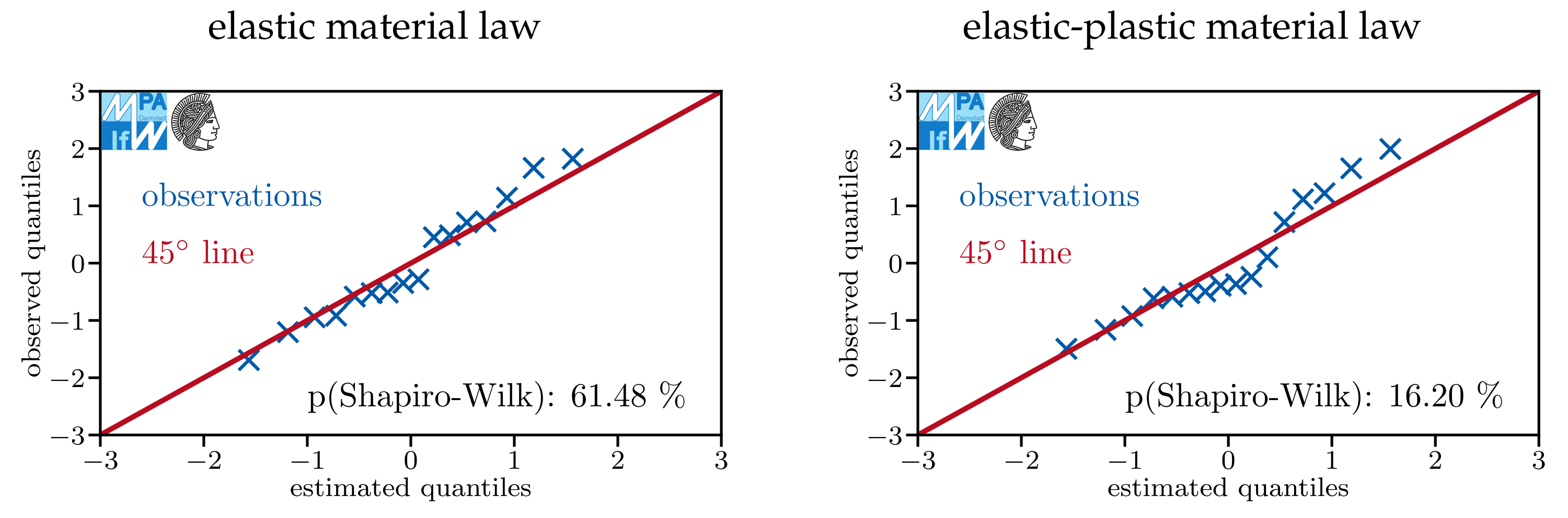
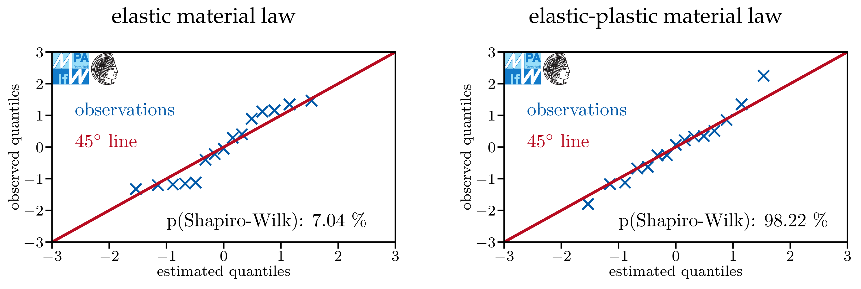
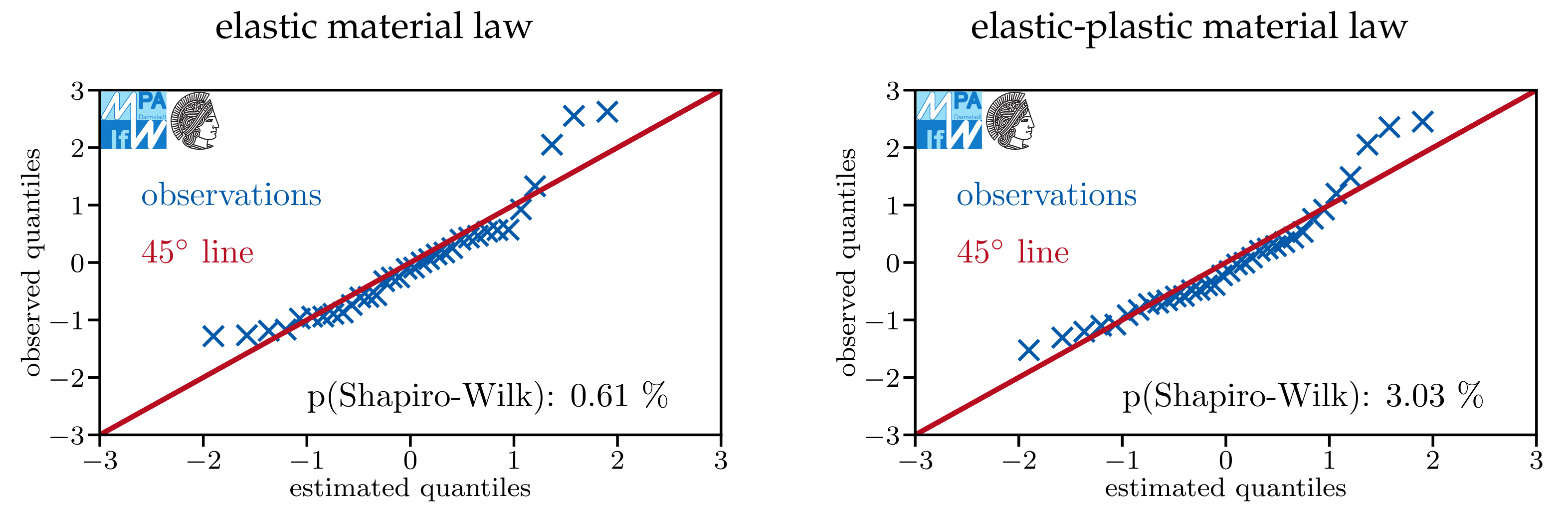
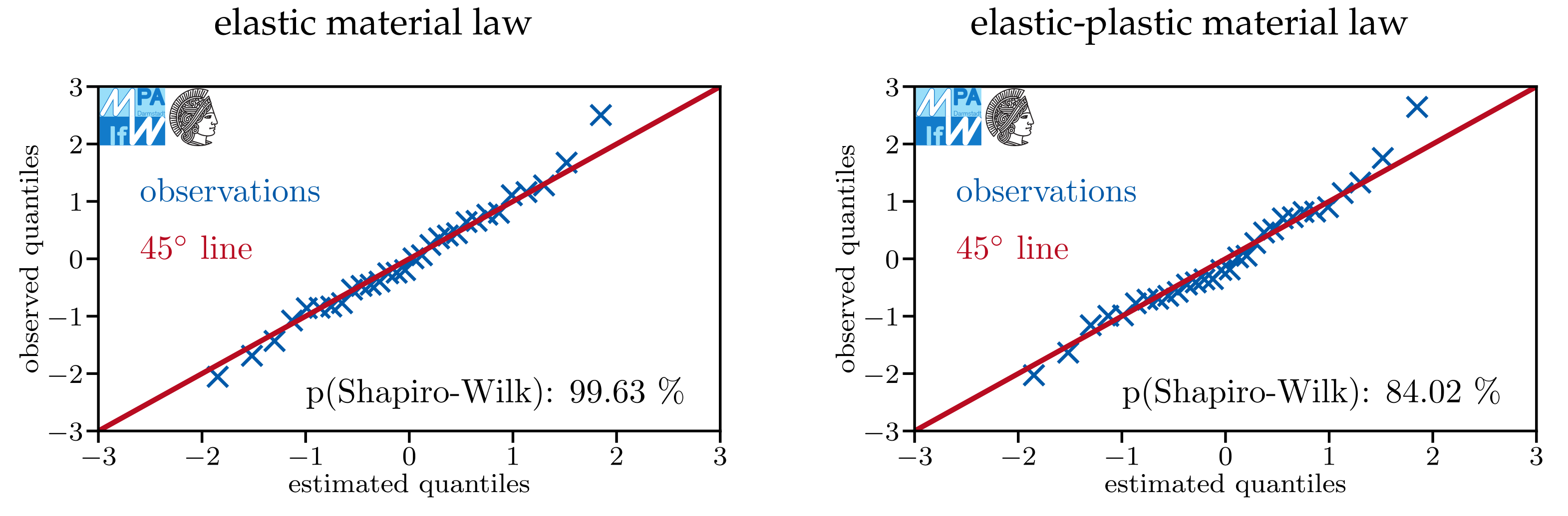
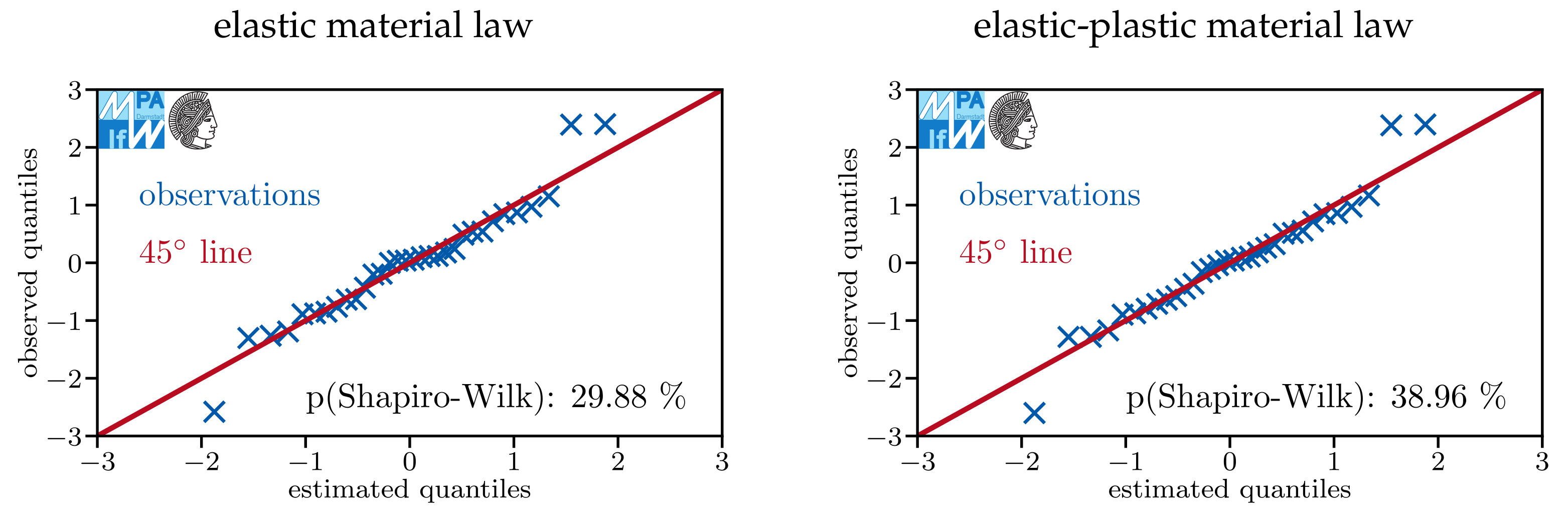
Appendix A. Do Models Assuming Log-Normal Distributions Describe the Data Sets Well?


References
- Dowling, N.E. Mechanical Behavior of Materials: Engineering Methods for Deformation, Fracture, and Fatigue; Pearson: Boston, MA, USA, 2012. [Google Scholar]
- Bathias, C. There is no infinite fatigue life in metallic materials. Fatigue Fract. Eng. Mater. Struct. 1999, 22, 559–565. [Google Scholar] [CrossRef]
- Bathias, C.; Drouillac, L.; Le Francois, P. How and why the fatigue S-N curve does not approach a horizontal asymptote. Int. J. Fatigue 2001, 23, 143–151. [Google Scholar] [CrossRef]
- Schwerdt, D. Schwingfestigkeit und Schädigungsmechanismen der Aluminiumlegierungen EN AW-6056 und EN AW-6082 sowie des Vergütungsstahls 42CrMo4 bei sehr hohen Schwingspielzahlen; TU Darmstadt: Darmstadt, Germany, 2011. [Google Scholar]
- Oechsner, M.; Hanselka, H.; Schneider, N.; Eufinger, J.; Pyttel, B.; Berger, C. Schlussbericht zu BMWi 324 ZN: Bauteilauslegung unter Berücksichtigung von Beanspruchungen mit variablen Amplituden und sehr hohen Schwingspielzahlen; MPA-IfW—Technische Universität Darmstadt: Darmstadt, Germany, 2012. [Google Scholar]
- Schneider, N. Ermüdungsfestigkeit bei sehr hohen Schwingspielzahlen unter Berücksichtigung des Einflusses der Prüffrequenz. Ph.D. Thesis, TU Darmstadt, Darmstadt, Germany, 2014. [Google Scholar]
- Schneider, N.; Schwerdt, D.; Wuttke, U.; Oechsner, M. Fatigue at high number of cyclic loads: Testing methods and failure mechanism. Mater. Und Werkst. 2015, 46, 931–941. [Google Scholar] [CrossRef]
- Krupp, U.; Giertler, A.; Koschella, K. Microscopic Damage Evolution During Very High Cycle Fatigue (VHCF) of Tempered Martensitic Steel. Procedia Eng. 2016, 160, 231–238. [Google Scholar] [CrossRef][Green Version]
- Schneider, N.; Bödecker, J.; Berger, C.; Oechsner, M. Frequency effect and influence of testing technique on the fatigue behaviour of quenched and tempered steel and aluminium alloy. Int. J. Fatigue 2016, 93, 224–231. [Google Scholar] [CrossRef]
- Oechsner, M.; Melz, T.; Kaffenberger, M.; Störzel, K. Schlussbericht zu AiF A 18198 N: Bauteilauslegung unter Berücksichtigung von Beanspruchungen mit variablen Amplituden und sehr hohen Schwingspielzahlen; MPA-IfW—Technische Universität Darmstadt: Darmstadt, Germany, 2017. [Google Scholar]
- Pyttel, B.; Brunner, I.; Kaiser, B.; Berger, C.; Mahendran, M. Fatigue behaviour of helical compression springs at a very high number of cycles—Investigation of various influences. Int. J. Fatigue 2014, 60, 101–109. [Google Scholar] [CrossRef]
- Pyttel, B.; Fernández Canteli, A.; Argente Ripoll, A. Comparison of different statistical models for description of fatigue including very high cycle fatigue. Int. J. Fatigue 2016, 93, 435–442. [Google Scholar] [CrossRef]
- Mayer, H.; Schuller, R.; Karr, U.; Fitzka, M.; Irrasch, D.; Hahn, M.; Bacher-Höchst, M. Mean stress sensitivity and crack initiation mechanisms of spring steel for torsional and axial VHCF loading. Int. J. Fatigue 2016, 93, 309–317. [Google Scholar] [CrossRef]
- Mayer, H. Recent developments in ultrasonic fatigue. Fatigue Fract. Eng. Mater. Struct. 2016, 39, 3–29. [Google Scholar] [CrossRef]
- Jeddi, D.; Palin-Luc, T. A review about the effects of structural and operational factors on the gigacycle fatigue of steels. Fatigue Fract. Eng. Mater. Struct. 2018, 41, 969–990. [Google Scholar] [CrossRef]
- Bach, J. Ermüdungsverhalten von Niedrig Legierten Stählen im HCF-und VHCF-Bereich. Ph.D. Thesis, Friedrich-Alexander-Universität Erlangen-Nürnberg, Erlangen, Germany, 2018. [Google Scholar]
- Bach, J.; Göken, M.; Höppel, H.W. Fatigue of low alloyed carbon steels in the HCF/VHCF-regimes. In Fatigue of Materials at Very High Numbers of Loading Cycles; Springer Fachmedien Wiesbaden: Wiesbaden, Germany, 2018; pp. 1–23. [Google Scholar]
- Cai, Y.; Zhao, Y.; Ma, X.; Yang, Z.; Ding, Y. An extended model for fatigue life prediction and acceleration considering load frequency effect. IEEE Access 2018, 6, 21064–21074. [Google Scholar] [CrossRef]
- Hu, Y.; Sun, C.; Xie, J.; Hong, Y. Effects of loading frequency and loading type on high-cycle and very-high-cycle fatigue of a high-strength steel. Materials 2018, 11, 1456. [Google Scholar] [CrossRef] [PubMed]
- Geilen, M.B.; Klein, M.; Oechsner, M. Very high cycle fatigue behaviour of compression springs under constant and variable amplitude loading. Mater. Und Werkst. 2019, 50, 1301–1316. [Google Scholar] [CrossRef]
- Geilen, M.B.; Klein, M.; Oechsner, M.; Kaffenberger, M.; Störzel, K.; Melz, T. A Method for the Strain Rate Dependent Correction for Control Type of Fatigue Tests. Int. J. Fatigue 2020, 138, 105726. [Google Scholar] [CrossRef]
- Atrens, A.; Hoffelner, W.; Duerig, T.W.; Allison, J.E. Subsurface crack initiation in high cycle fatigue in Ti6A14V and in a typical martensitic stainless steel. Scr. Metall. 1983, 17, 601–606. [Google Scholar] [CrossRef]
- Furuya, Y.; Matsuoka, S.; Abe, T.; Yamaguchi, K. Gigacycle fatigue properties for high-strength low-alloy steel at 100 Hz, 600 Hz, and 20 kHz. Scr. Mater. 2002, 46, 157–162. [Google Scholar] [CrossRef]
- Furuya, Y.; Matsuoka, S. Gigacycle fatigue properties of a modified-ausformed Si-Mn steel and effects of microstructure. Metall. Mater. Trans. A 2004, 35, 1715–1723. [Google Scholar] [CrossRef]
- Tsutsumi, N.; Murakami, Y.; Doquet, V. Effect of test frequency on fatigue strength of low carbon steel. Fatigue Fract. Eng. Mater. Struct. 2009, 32, 473–483. [Google Scholar] [CrossRef]
- Müller-Bollenhagen, C.; Zimmermann, M.; Christ, H.J. Adjusting the very high cycle fatigue properties of a metastable austenitic stainless steel by means of the martensite content. Procedia Eng. 2010, 2, 1663–1672. [Google Scholar] [CrossRef]
- Pyttel, B.; Schwerdt, D.; Berger, C. Fatigue strength and failure mechanisms in the VHCF-region for quenched and tempered steel 42CrMoS4 and consequences to fatigue design. Procedia Eng. 2010, 2, 1327–1336. [Google Scholar] [CrossRef]
- Setowaki, S.; Ichikawa, Y.; Nonaka, I. Effect of frequency on high cycle fatigue strength of railway axle steel. Proceedings of fifth International Conference on Very High Cycle Fatigue VHCF5, Berlin, Germany, 28–30 June 2011; pp. 153–158. [Google Scholar]
- Nonaka, I.; Setowaki, S.; Ichikawa, Y. Effect of load frequency on high cycle fatigue strength of bullet train axle steel. Int. J. Fatigue 2014, 60, 43–47. [Google Scholar] [CrossRef]
- Guennec, B.; Ueno, A.; Sakai, T.; Takanashi, M.; Itabashi, Y. Effect of the loading frequency on fatigue properties of JIS S15C low carbon steel and some discussions based on micro-plasticity behavior. Int. J. Fatigue 2014, 66, 29–38. [Google Scholar] [CrossRef]
- Zhu, M.L.; Liu, L.L.; Xuan, F.Z. Effect of frequency on very high cycle fatigue behavior of a low strength Cr–Ni–Mo–V steel welded joint. Int. J. Fatigue 2015, 77, 166–173. [Google Scholar] [CrossRef]
- Torabian, N.; Favier, V.; Dirrenberger, J.; Adamski, F.; Ziaei-Rad, S.; Ranc, N. Correlation of the high and very high cycle fatigue response of ferrite based steels with strain rate-temperature conditions. Acta Mater. 2017, 134, 40–52. [Google Scholar] [CrossRef]
- Mayer, H.; Papakyriacou, M.; Pippan, R.; Stanzl-Tschegg, S. Influence of loading frequency on the high cycle fatigue properties of AlZnMgCu1. 5 aluminium alloy. Mater. Sci. Eng. A 2001, 314, 48–54. [Google Scholar] [CrossRef]
- Papakyriacou, M.; Mayer, H.; Pypen, C.; Plenk, H., Jr.; Stanzl-Tschegg, S. Influence of loading frequency on high cycle fatigue properties of bcc and hcp metals. Mater. Sci. Eng. A 2001, 308, 143–152. [Google Scholar] [CrossRef]
- Mayer, H.; Ede, C.; Allison, J.E. Influence of cyclic loads below endurance limit or threshold stress intensity on fatigue damage in cast aluminium alloy 319-T7. Int. J. Fatigue 2005, 27, 129–141. [Google Scholar] [CrossRef]
- Engler-Pinto, C.C., Jr.; Frisch Sr, R.J.; Lasecki, J.V.; Mayer, H.; Allison, J.E. Effect of frequency and environment on high cycle fatigue of cast aluminum alloys. In Proceedings of the VHCF-Fourth International Conference on Very High Cycle Fatigue, Ann Arbor, MI, USA, 19–22 August 2007; pp. 421–427. [Google Scholar]
- Takeuchi, E.; Furuya, Y.; Nagashima, N.; Matsuoka, S. The effect of frequency on the giga–cycle fatigue properties of a Ti–6Al–4V alloy. Fatigue Fract. Eng. Mater. Struct. 2008, 31, 599–605. [Google Scholar] [CrossRef]
- Zhu, X.; Jones, J.W.; Allison, J.E. Effect of frequency, environment, and temperature on fatigue behavior of E319 cast aluminum alloy: Stress-controlled fatigue life response. Metall. Mater. Trans. A 2008, 39, 2681–2688. [Google Scholar] [CrossRef]
- Begum, S.; Chen, D.L.; Xu, S.; Luo, A.A. Effect of strain ratio and strain rate on low cycle fatigue behavior of AZ31 wrought magnesium alloy. Mater. Sci. Eng. A 2009, 517, 334–343. [Google Scholar] [CrossRef]
- Protz, R.; Kosmann, N.; Gude, M.; Hufenbach, W.; Schulte, K.; Fiedler, B. Voids and their effect on the strain rate dependent material properties and fatigue behaviour of non-crimp fabric composites materials. Compos. Part B Eng. 2015, 83, 346–351. [Google Scholar] [CrossRef]
- Jost, B.; Klein, M.; Beck, T.; Eifler, D. Temperature dependent cyclic deformation and fatigue life of EN-GJS-600 (ASTM 80-55-06) ductile cast iron. Int. J. Fatigue 2017, 96, 102–113. [Google Scholar] [CrossRef]
- Jost, B.; Klein, M.; Beck, T.; Eifler, D. Temperature and frequency influence on the cyclic deformation behavior of EN-GJS-600 (ASTM 80-55-06) ductile cast iron at 0.005 and 5 Hz. Int. J. Fatigue 2018, 110, 225–237. [Google Scholar] [CrossRef]
- Wang, M.; Pang, J.C.; Liu, H.Q.; Zou, C.L.; Li, S.X.; Zhang, Z.F. Deformation mechanism and fatigue life of an Al-12Si alloy at different temperatures and strain rates. Int. J. Fatigue 2019, 127, 268–274. [Google Scholar] [CrossRef]
- Campbell, J.D.; Ferguson, W.G. The temperature and strain-rate dependence of the shear strength of mild steel. Philos. Mag. 1970, 21, 63–82. [Google Scholar] [CrossRef]
- Jaske, C.E.; Leis, B.N.; Pugh, C.E. Monotonic and Cyclic Stress-Strain Response of Annealed 2 1/4 Cr–1 Mo Steel; Oak Ridge National Lab: Oak Ridge, TN, USA, 1975. [Google Scholar]
- El-Magd, E. Influence of strain rate on ductility of metallic materials. Steel Res. 1997, 68, 67–71. [Google Scholar] [CrossRef]
- Bleck, W.; Schael, I. Determination of crash–relevant material parameters by dynamic tensile tests. Steel Res. 2000, 71, 173–178. [Google Scholar] [CrossRef]
- Børvik, T.; Hopperstad, O.S.; Berstad, T. On the influence of stress triaxiality and strain rate on the behaviour of a structural steel. Part II. Numerical study. Eur. J. Mech.-A/Solids 2003, 22, 15–32. [Google Scholar] [CrossRef]
- Hopperstad, O.S.; Børvik, T.; Langseth, M.; Labibes, K.; Albertini, C. On the influence of stress triaxiality and strain rate on the behaviour of a structural steel. Part I. Experiments. Eur. J. Mech.-A/Solids 2003, 22, 1–13. [Google Scholar] [CrossRef]
- Lee, W.S.; Liu, C.Y. The effects of temperature and strain rate on the dynamic flow behaviour of different steels. Mater. Sci. Eng. A 2006, 426, 101–113. [Google Scholar] [CrossRef]
- Böhme, W.; Luke, M.; Blauel, J.G.; Sun, D.-Z.; Rohr, I.; Harwick, W. FAT-Richtlinie Dynamische Werkstoffkennwerte für die Crashsimulation; FAT-Schriftenreihe: Frankfurt am Main, Germany, 2007; Volume 211. [Google Scholar]
- Emde, T. Mechanisches Verhalten metallischer Werkstoffe über weite Bereiche der Dehnung, der Dehnrate und der Temperatur; Verlagshaus Mainz GmbH: Aachen, Germany, 2009. [Google Scholar]
- Benson, D.K.; Hancock, J.R. The effect of strain rate on the cyclic response of metals. Metall. Trans. 1974, 5, 1711–1715. [Google Scholar] [CrossRef]
- Pineau, A.; Benzerga, A.A.; Pardoen, T. Failure of metals I: Brittle and ductile fracture. Acta Mater. 2016, 107, 424–483. [Google Scholar] [CrossRef]
- Hodowany, J.; Ravichandran, G.; Rosakis, A.J.; Rosakis, P. Partition of plastic work into heat and stored energy in metals. Exp. Mech. 2000, 40, 113–123. [Google Scholar] [CrossRef]
- Cho, K.M.; Lee, S.; Nutt, S.R.; Duffy, J. Adiabatic shear band formation during dynamic torsional deformation of an HY-100 steel. Acta Metall. Mater. 1993, 41, 923–932. [Google Scholar] [CrossRef]
- Kapoor, R.; Nemat-Nasser, S. Determination of temperature rise during high strain rate deformation. Mech. Mater. 1998, 27, 1–12. [Google Scholar] [CrossRef]
- Rosakis, P.; Rosakis, A.J.; Ravichandran, G.; Hodowany, J. A thermodynamic internal variable model for the partition of plastic work into heat and stored energy in metals. J. Mech. Phys. Solids 2000, 48, 581–607. [Google Scholar] [CrossRef]
- Holzer, A.J.; Brown, R.H. Mechanical behavior of metals in dynamic compression. J. Eng. Mater. Technol. 1979, 101, 238–247. [Google Scholar] [CrossRef]
- Klepaczko, J.R. An experimental technique for shear testing at high and very high strain rates. The case of a mild steel. Int. J. Impact Eng. 1994, 15, 25–39. [Google Scholar] [CrossRef]
- Johnson, G.R.; Cook, W.H. Fracture characteristics of three metals subjected to various strains, strain rates, temperatures and pressures. Eng. Fract. Mech. 1985, 21, 31–48. [Google Scholar] [CrossRef]
- Zerbst, U.; Vormwald, M.; Pippan, R.; Gänser, H.P.; Sarrazin-Baudoux, C.; Madia, M. About the fatigue crack propagation threshold of metals as a design criterion–a review. Eng. Fract. Mech. 2016, 153, 190–243. [Google Scholar] [CrossRef]
- Tanaka, H.; Homma, N.; Matsuoka, S.; Murakami, Y. Effect of hydrogen and frequency on fatigue behavior of SCM435 steel for storage cylinder of hydrogen station. Nihon Kikai Gakkai Ronbunshu Hen/Trans. Jpn. Soc. Mech. Eng. Part A 2007, 73, 1358–1365. [Google Scholar]
- Murakami, Y.; Matsuoka, S. Effect of hydrogen on fatigue crack growth of metals. Eng. Fract. Mech. 2010, 77, 1926–1940. [Google Scholar] [CrossRef]
- Suresh, S.; Ritchie, R.O. Near-threshold fatigue crack propagation: A perspective on the role of crack closure. In Fatigue Crack Growth Threshold Concepts; The Metallurgical Society Inc.: Warrendale, PA, USA, 1983. [Google Scholar]
- Blom, A.F.; Holm, D.K. An experimental and numerical study of crack closure. Eng. Fract. Mech. 1985, 22, 997–1011. [Google Scholar] [CrossRef]
- Vasudeven, A.K.; Sadananda, K.; Louat, N. A review of crack closure, fatigue crack threshold and related phenomena. Mater. Sci. Eng. A 1994, 188, 1–22. [Google Scholar] [CrossRef]
- Chermahini, R.G.; Shivakumar, K.N.; Newman, J.C., Jr.; Blom, A.F. Three-dimensional aspects of plasticity-induced fatigue crack closure. Eng. Fract. Mech. 1989, 34, 393–401. [Google Scholar] [CrossRef]
- Pippan, R.; Hohenwarter, A. Fatigue crack closure: A review of the physical phenomena. Fatigue Fract. Eng. Mater. Struct. 2017, 40, 471–495. [Google Scholar] [CrossRef]
- Jiang, Y.; Feng, M.; Ding, F. A reexamination of plasticity-induced crack closure in fatigue crack propagation. Int. J. Plast. 2005, 21, 1720–1740. [Google Scholar] [CrossRef]
- Weibull, W. A Statistical Theory of Strength of Materials; Generalstabens litografiska anstalts förlag: Stockholm, Sweden, 1939. [Google Scholar]
- Kuhn, P. Effect of geometric size on notch fatigue. In Colloquium on Fatigue; Springer: Berlin/Heidelberg, Germany, 1956; pp. 131–140. [Google Scholar]
- Böhm, J.; Heckel, K. Die Vorhersage der Dauerschwingfestigkeit unter Berücksichtigung des statistischen Größeneinflusses. Mater. Und Werkst. 1982, 13, 120–128. [Google Scholar] [CrossRef]
- Liu, J.; Zenner, H. Berechnung der Dauerschwingfestigkeit unter Berücksichtigung der spannungsmechanischen und statistischen Stützziffer. Mater. Und Werkst. 1991, 22, 187–196. [Google Scholar] [CrossRef]
- Liu, J.; Zenner, H. Berechnung von Bauteilwöhlerlinien unter Berücksichtigung der statistischen und spannungsmechanischen Stützziffer. Mater. Und Werkst. 1995, 26, 14–21. [Google Scholar] [CrossRef]
- Kloos, K.H.; Kaiser, B.; Friederich, H. Einfluß der Probengröße auf das Verformungs–und Versagensverhalten von Vergütungsstahl 42 CrMo 4 unter Schwingbeanspruchung. Mater. Und Werkst. 1995, 26, 330–336. [Google Scholar] [CrossRef]
- Friederich, H.; Kaiser, B.; Kloos, K.H. Anwendung der Fehlstellentheorie nach Weibull zur Berechnung des statistischen Größeneinflusses bei Dauerschwingbeanspruchung. Mater. Und Werkst. 1998, 29, 178–184. [Google Scholar] [CrossRef]
- Bomas, H.; Linkewitz, T.; Mayr, P. Application of a weakest–link concept to the fatigue limit of the bearing steel SAE 52100 in a bainitic condition. Fatigue Fract. Eng. Mater. Struct. 1999, 22, 733–741. [Google Scholar] [CrossRef]
- Makkonen, M. Statistical size effect in the fatigue limit of steel. Int. J. Fatigue 2001, 23, 395–402. [Google Scholar] [CrossRef]
- Flacelière, L.; Morel, F. Probabilistic approach in high–cycle multiaxial fatigue: Volume and surface effects. Fatigue Fract. Eng. Mater. Struct. 2004, 27, 1123–1135. [Google Scholar] [CrossRef]
- Castillo, E.; Fernandez-Canteli, A. A Unified Statistical Methodology for Modeling Fatigue Damage; Springer Science & Business Media: Berlin/Heildelberg, Germay, 2009. [Google Scholar]
- Hertel, O.; Vormwald, M. Statistical and geometrical size effects in notched members based on weakest-link and short-crack modelling. Eng. Fract. Mech. 2012, 95, 72–83. [Google Scholar] [CrossRef]
- Ai, Y.; Zhu, S.P.; Liao, D.; Correia, J.A.; de Jesus, A.M.P.; Keshtegar, B. Probabilistic modelling of notch fatigue and size effect of components using highly stressed volume approach. Int. J. Fatigue 2019, 127, 110–119. [Google Scholar] [CrossRef]
- Vaara, J.; Väntänen, M.; Kämäräinen, P.; Kemppainen, J.; Frondelius, T. Bayesian analysis of critical fatigue failure sources. Int. J. Fatigue 2020, 130, 105282. [Google Scholar] [CrossRef]
- Rennert, R.; Kullig, E.; Vormwald, M.; Esderts, A.; Siegele, D. Rechnerischer Festigkeitsnachweis für Maschinenbauteile aus Stahl, Eisenguss- und Aluminiumwerkstoffen, 6th ed.; FKM-Richtlinie, VDMA Verlag: Frankfurt am Main, Germany, 2012. [Google Scholar]
- Fiedler, M.; Wächter, M.; Varfolomeev, I.; Vormwald, M.; Esderts, A. Rechnerischer Festigkeitsnachweis unter Expliziter Erfassung Nichtlinearen Werkstoffverhaltens für Maschinenbauteile aus Stahl, Stahlguss und Aluminiumknetlöegierungen, 1st ed.; FKM-Richtlinie, VDMA Verlag: Frankfurt am Main, Germany, 2019. [Google Scholar]
- Kletzin, U.; Reich, R.; Oechsner, M.; Spies, A.; Pyttel, B.; Hanning, G.; Rennert, R.; Kullig, E. Rechnerischer Festigkeitsnachweis für Federn und Federelemente, 1st ed.; FKM-Richtlinie, VDMA Verlag: Frankfurt am Main, Germany, 2020. [Google Scholar]
- Skelton, R.P.; Haigh, J.R. Fatigue crack growth rates and thresholds in steels under oxidising conditions. Mater. Sci. Eng. 1978, 36, 17–25. [Google Scholar] [CrossRef]
- Suresh, S.; Zamiski, G.F.; Ritchie, D.R.O. Oxide-induced crack closure: An explanation for near-threshold corrosion fatigue crack growth behavior. Metall. Mater. Trans. A 1981, 12, 1435–1443. [Google Scholar] [CrossRef]
- Liaw, P.K.; Leax, T.R.; Williams, R.S.; Peck, M.G. Influence of oxide-induced crack closure on near-threshold fatigue crack growth behavior. Acta Metall. 1982, 30, 2071–2078. [Google Scholar] [CrossRef]
- Maierhofer, J.; Simunek, D.; Gänser, H.P.; Pippan, R. Oxide induced crack closure in the near threshold regime: The effect of oxide debris release. Int. J. Fatigue 2018, 117, 21–26. [Google Scholar] [CrossRef]
- Riemelmoser, F.O.; Gumbsch, P.; Pippan, R. Dislocation modelling of fatigue cracks: An overview. Mater. Trans. 2001, 42, 2–13. [Google Scholar] [CrossRef]
- Lee, H.H.; Uhlig, H.H. Corrosion fatigue of type 4140 high strength steel. Metall. Mater. Trans. B 1972, 3, 2949–2957. [Google Scholar] [CrossRef]
- Shives, T.R.; Bennett, J.A. The Effect of Environment on the Fatigue Strengths of Four Selected Alloys; National Aeronautics and Space Administration: Washington, DC, USA, 1965. [Google Scholar]
- Wadsworth, N.J. The influence of atmospheric corrosion on the fatigue limit of iron-0.5% carbon. Philos. Mag. 1961, 6, 397–401. [Google Scholar] [CrossRef]
- Yoshinaka, F.; Nakamura, T. Effect of vacuum environment on fatigue fracture surfaces of high strength steel. Mech. Eng. Lett. 2016, 2, 15–00730. [Google Scholar] [CrossRef][Green Version]
- Spriestersbach, D. VHCF-Verhalten des hochfesten Stahls 100Cr6: Rissinitiierungsmechanismen und Schwellenwerte. Ph.D. Thesis, TU Kaiserslaurtern, Kaiserslautern, Germany, 2020. [Google Scholar]
- Wei, R.; Talda, P.; Li, C.Y. Fatigue-crack propagation in some ultrahigh-strength steels. In Fatigue Crack Propagation; ASTM International: West Conshohocken, PA, USA, 1967. [Google Scholar]
- Dahlberg, E.P. Fatigue-crack propagation in high-strength 4340 steel in humid air(Water vapor effects on fatigue crack propagation rates in high strength 4340 steel examined by optical and electron fractography). ASM Trans. Q. 1965, 58, 46–53. [Google Scholar]
- Achter, M. Effect of environment on fatigue cracks. In Fatigue Crack Propagation; ASTM International: West Conshohocken, PA, USA, 1967. [Google Scholar]
- Henaff, G.; Marchal, K.; Petit, J. On fatigue crack propagation enhancement by a gaseous atmosphere: experimental and theoretical aspects. Acta Metall. Mater. 1995, 43, 2931–2942. [Google Scholar] [CrossRef]
- Spriestersbach, D.; Grad, P.; Brodyanski, A.; Lösch, J.; Kopnarski, M.; Kerscher, E. Very high cycle fatigue crack initiation: Investigation of fatigue mechanisms and threshold values for 100Cr6. In Fatigue of Materials at Very High Numbers of Loading Cycles; Springer: Berlin, Germany, 2018; pp. 167–210. [Google Scholar]
- Thompson, N.; Wadsworth, N.J.; Louat, N. The origin of fatigue fracture in copper. Philos. Mag. 1956, 1, 113–126. [Google Scholar] [CrossRef]
- Duquette, D.J. Environmental Effects on General Fatigue Resistance and Crack Nucleation in Metals and Alloys; Technical Report; Office of Naval Research: Troy, NY, USA, 1978. [Google Scholar]
- Hudson, C.M.; Seward, S.K. A literature review and inventory of the effects of environment on the fatigue behavior of metals. Eng. Fract. Mech. 1976, 8, 315–329. [Google Scholar] [CrossRef]
- Krupp, U. Mikrostrukturelle Aspekte der Rissinitiierung und-ausbreitung in metallischen Werkstoffen. Habilitation Thesis, Universität Siegen, Siegen, Germany, 2004. [Google Scholar]
- Bradhurst, D.H.; Leach, J.L. The mechanical properties of thin anodic films on aluminum. J. Electrochem. Soc. 1966, 113, 1245. [Google Scholar] [CrossRef]
- Grosskreutz, J.C. The effect of oxide films on dislocation-surface interactions in aluminum. Surf. Sci. 1967, 8, 173–190. [Google Scholar] [CrossRef]
- Nakamura, T.; Oguma, H.; Shinohara, Y. The effect of vacuum-like environment inside sub-surface fatigue crack on the formation of ODA fracture surface in high strength steel. Procedia Eng. 2010, 2, 2121–2129. [Google Scholar] [CrossRef]
- Petit, J.; Sarrazin-Baudoux, C. An overview on the influence of the atmosphere environment on ultra-high-cycle fatigue and ultra-slow fatigue crack propagation. Int. J. Fatigue 2006, 28, 1471–1478. [Google Scholar] [CrossRef]
- Murakami, Y.; Nomoto, T.; Ueda, T.; Murakami, Y. On the mechanism of fatigue failure in the superlong life regime (N> 10000000 cycles). Part 1: Influence of hydrogen trapped by inclusions. Fatigue Fract. Eng. Mater. Struct. 2000, 23, 893–902. [Google Scholar] [CrossRef]
- Murakami, Y.; Nomoto, T.; Ueda, T.; Murakami, Y. On the mechanism of fatigue failure in the superlong life regime (N> 10000000 cycles). Part II: Influence of hydrogen trapped by inclusions. Fatigue Fract. Eng. Mater. Struct. 2000, 23, 903–910. [Google Scholar] [CrossRef]
- Barrera, O.; Tarleton, E.; Tang, H.W.; Cocks, A.C. Modelling the coupling between hydrogen diffusion and the mechanical behaviour of metals. Comput. Mater. Sci. 2016, 122, 219–228. [Google Scholar] [CrossRef]
- Barrera, O.; Bombac, D.; Chen, Y.; Daff, T.D.; Galindo-Nava, E.; Gong, P.; Haley, D.; Horton, R.; Katzarov, I.; Kermode, J.R. Understanding and mitigating hydrogen embrittlement of steels: A review of experimental, modelling and design progress from atomistic to continuum. J. Mater. Sci. 2018, 53, 6251–6290. [Google Scholar] [CrossRef]
- Giertler, A. Volume 2020, Band 2, Berichte aus dem Institut für Eisenhüttenkunde. In Mechanismen der Rissentstehung und -ausbreitung im Vergütungsstahl 50CrMo4 bei sehr hohen Lastspielzahlen; Shaker Verlag: Düren, Germany, 2020. [Google Scholar]
- Glaser, A. Mittelspannungseinfluß auf das Verformungsverhalten von Ck 45 und 42 CrMo 4 bei Spannungs-Und Dehnungskontrollierter Homogen-Einachsiger Schwingbeanspruchung. Ph.D. Thesis, KIT, Karlsruhe, Germany, 1988. [Google Scholar]
- Ramberg, W.; Osgood, W.R. Description of Stress-Strain Curves by Three Parameters; National Advisory Comitee for Aeronatuics: Washington, DC, USA, 1943. [Google Scholar]
- Neuber, H. Über die Berücksichtigung der Spannungskonzenlration bei Festigkeitsproblemen. Konstr. Berl. 1968, 20, 245–251. [Google Scholar]
- Topper, T.; Wetzel, R.M.; Morrow, J. Neuber’s Rule Applied to Fatigue of Notched Specimens; U.S. Naval Air Engineering Center: Philadelphia, PA, USA, 1967. [Google Scholar]
- Wächter, M. Zur Ermittlung von zyklischen Werkstoffkennwerten und Schädigungsparameterwöhlerlinien; Technische Universität Clausthal: Clausthal-Zellerfeld, Germany, 2016. [Google Scholar]
- Müller, C. Zur Statistischen Auswertung Experimenteller Wöhlerlinien; Universitätsbibliothek Clausthal: Clausthal-Zellerfeld, Germany, 2015. [Google Scholar]
- Müller, C.; Wächter, M.; Masendorf, R.; Esderts, A. Distribution functions for the linear region of the SN curve. Mater. Test. 2017, 59, 625–629. [Google Scholar] [CrossRef]
- Radaj, D.; Vormwald, M. Ermüdungsfestigkeit; Springer: Berlin, Germany, 2007. [Google Scholar]
- Virtanen, P.; Gommers, R.; Oliphant, T.E.; Haberland, M.; Reddy, T.; Cournapeau, D.; Burovski, E.; Peterson, P.; Weckesser, W.; Bright, J. SciPy 1.0–Fundamental Algorithms for Scientific Computing in Python. arXiv 2019, arXiv:1907.10121. [Google Scholar] [CrossRef]
- Geilen, M.B.; Klein, M.; Oechsner, M. On the Influence of Ultimate Number of Cycles on Lifetime Prediction for Compression Springs Manufactured from VDSiCr Class Spring Wire. Materials 2020, 13, 3222. [Google Scholar] [CrossRef]
- Bomas, H.; Burkart, K.; Zoch, H.W. Evaluation of S–N curves with more than one failure mode. Int. J. Fatigue 2011, 33, 19–22. [Google Scholar] [CrossRef]
- Paolino, D.S.; Chiangdussi, G.; Rosetto, M. A unified statistical model for S–N fatigue curves: Probabilistic definition. Fatigue Fract. Eng. Mater. Struct. 2013, 36, 187–201. [Google Scholar] [CrossRef]
- Haydn, W.; Schwabe, F. Ermittlung geschlossener probabilistischer Auslegungskennlinien für einstufige Schwingfestigkeitsbeanspruchungen vom LCF- bis VHCF-Bereich. Mater. Und Werkst. 2015, 46, 591–602. [Google Scholar] [CrossRef]
- Fernández-Canteli, A.; Blasón, S.; Pyttel, B.; Muniz-Calvente, M.; Castillo, E. Considerations about the existence or non-existence of the fatigue limit: Implications on practical design. Int. J. Fract. 2020, 223, 189–196. [Google Scholar] [CrossRef]
- Muniz-Calvente, M.; Fernández-Canteli, A.; Pyttel, B.; Castillo, E. Probabilistic assessment of VHCF data as pertaining to concurrent populations using a Weibull regression model. Fatigue Fract. Eng. Mater. Struct. 2017, 40, 1772–1782. [Google Scholar] [CrossRef]
- Kobelev, V. A proposal for unification of fatigue crack growth. J. Phys. Conf. Ser. 2018, 843, 012022. [Google Scholar] [CrossRef]


| Material Batch | C | Cr | Mo | Mn | P | S |
|---|---|---|---|---|---|---|
| 919 MPa [5] | 0.53 | 1.06 | 0.19 | 0.69 | <0.01 | <0.01 |
| 1096 MPa [8] | 0.48 | 1.00 | 0.18 | 0.71 | 0.013 | 0.010 |
| 1170 MPa [10] | 0.49 | 1.01 | 0.19 | 0.69 | <0.01 | 0.011 |
| 1475 MPa [10] | 0.48 | 1.06 | 0.19 | 0.68 | 0.01 | 0.012 |
| 1726 MPa [6] | 0.51 | 1.09 | 0.19 | 0.73 | 0.016 | <0.01 |
| Material Batch | Young’s Modulus E in GPa | 0.2% Offset Yield Strength in MPa | Ultimate Tensile Strength in MPa |
|---|---|---|---|
| 919 MPa [5] | 206 | 842 | 919 |
| 1096 MPa [8] | 202 | 1000 | 1096 |
| 1170 MPa [10] | 208 | 1025 | 1170 |
| 1475 MPa [10] | 204 | 1345 | 1475 |
| 1726 MPa [6] | 215 | 1544 | 1726 |
| Material Batch | Young’s Modulus E in GPa | Hardening Coefficient in MPa | Hardening Exponent |
|---|---|---|---|
| 919 MPa | 206 | 1341 | 0.135 |
| 1096 MPa | 202 | 2816 | 0.237 |
| 1170 MPa | 204 | 1162 | 0.068 |
| 1475 MPa | 204 | 1436 | 0.073 |
| 1726 MPa | 215 | 1687 | 0.060 |
| Atmosphere | Corrected? | |||||||||
|---|---|---|---|---|---|---|---|---|---|---|
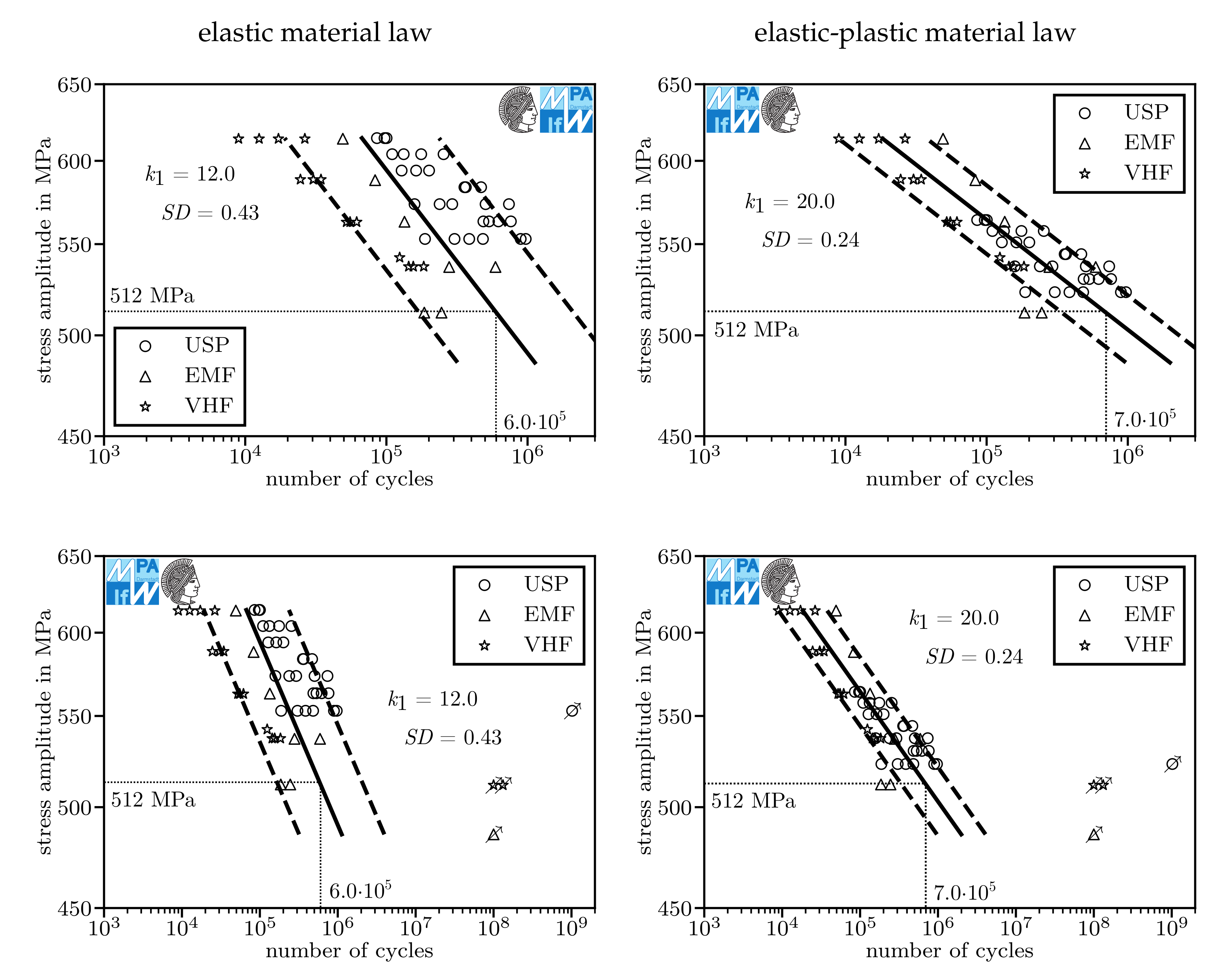
| Figure 8 | 919 MPa | 1 | lab air | no | 512 MPa | 6.0×10 | 12.0 | 0.43 | −28.4 | 50 |
| Figure 8 | 919 MPa | 1 | lab air | yes | 512 MPa | 7.0×10 | 20.0 | 0.24 | −0.4 | |
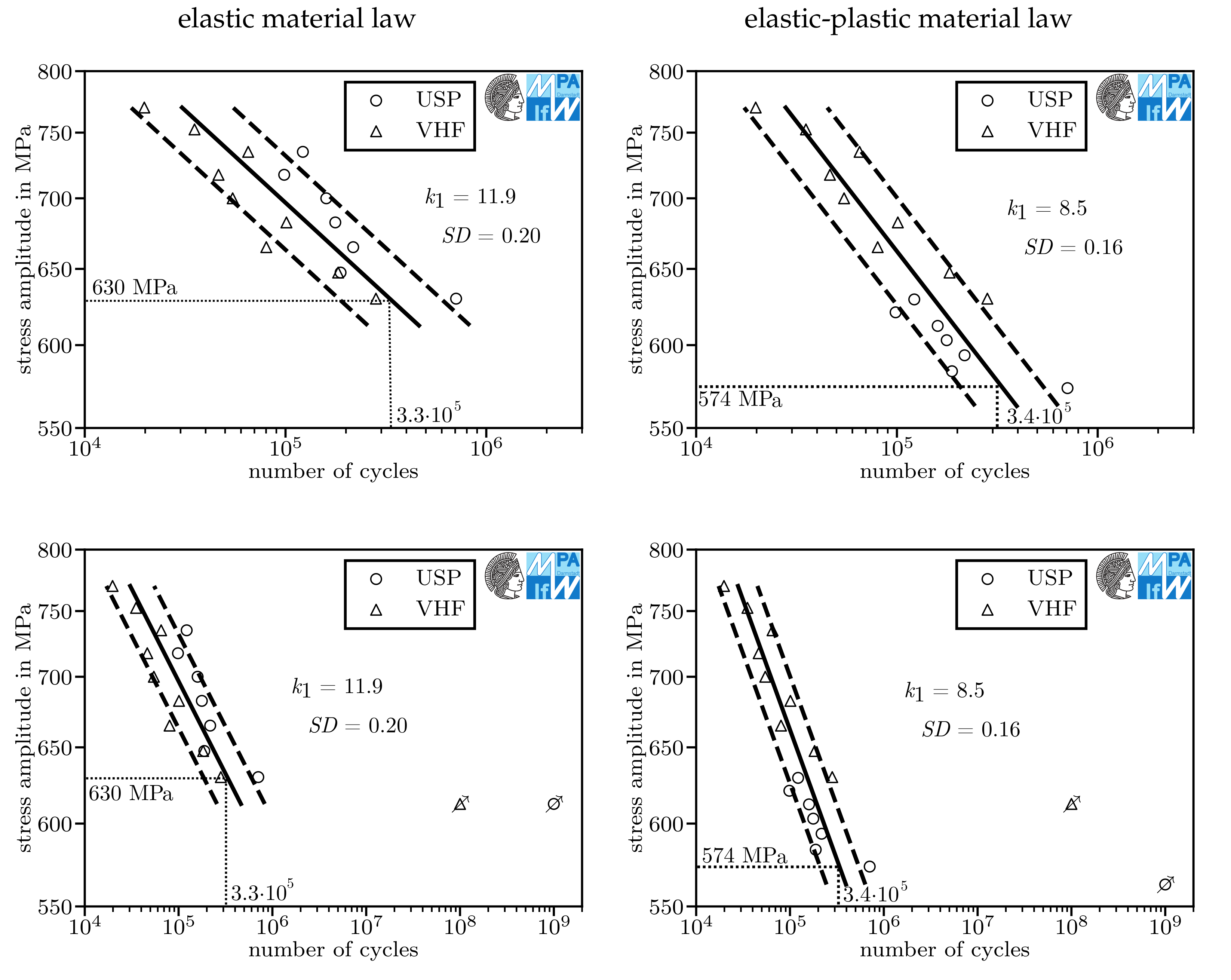
| Figure 9 | 919 MPa | 1.75 | lab air | no | 630 MPa | 3.3×10 | 11.9 | 0.20 | 3.2 | 16 |
| Figure 9 | 919 MPa | 1.75 | lab air | yes | 574 MPa | 3.4×10 | 8.5 | 0.16 | 6.5 | |
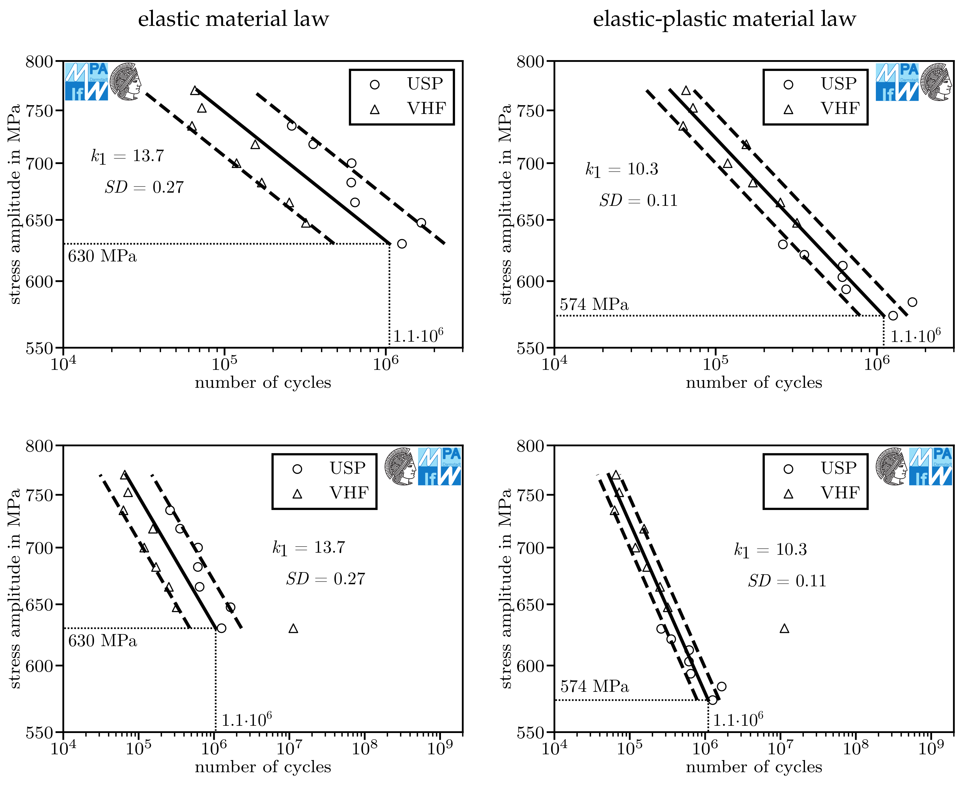
| Figure 10 | 919 MPa | 1.75 | argon | no | 630 MPa | 1.1×10 | 13.7 | 0.27 | −1.5 | 16 |
| Figure 10 | 919 MPa | 1.75 | argon | yes | 574 MPa | 1.1×10 | 10.3 | 0.11 | 11.2 | |
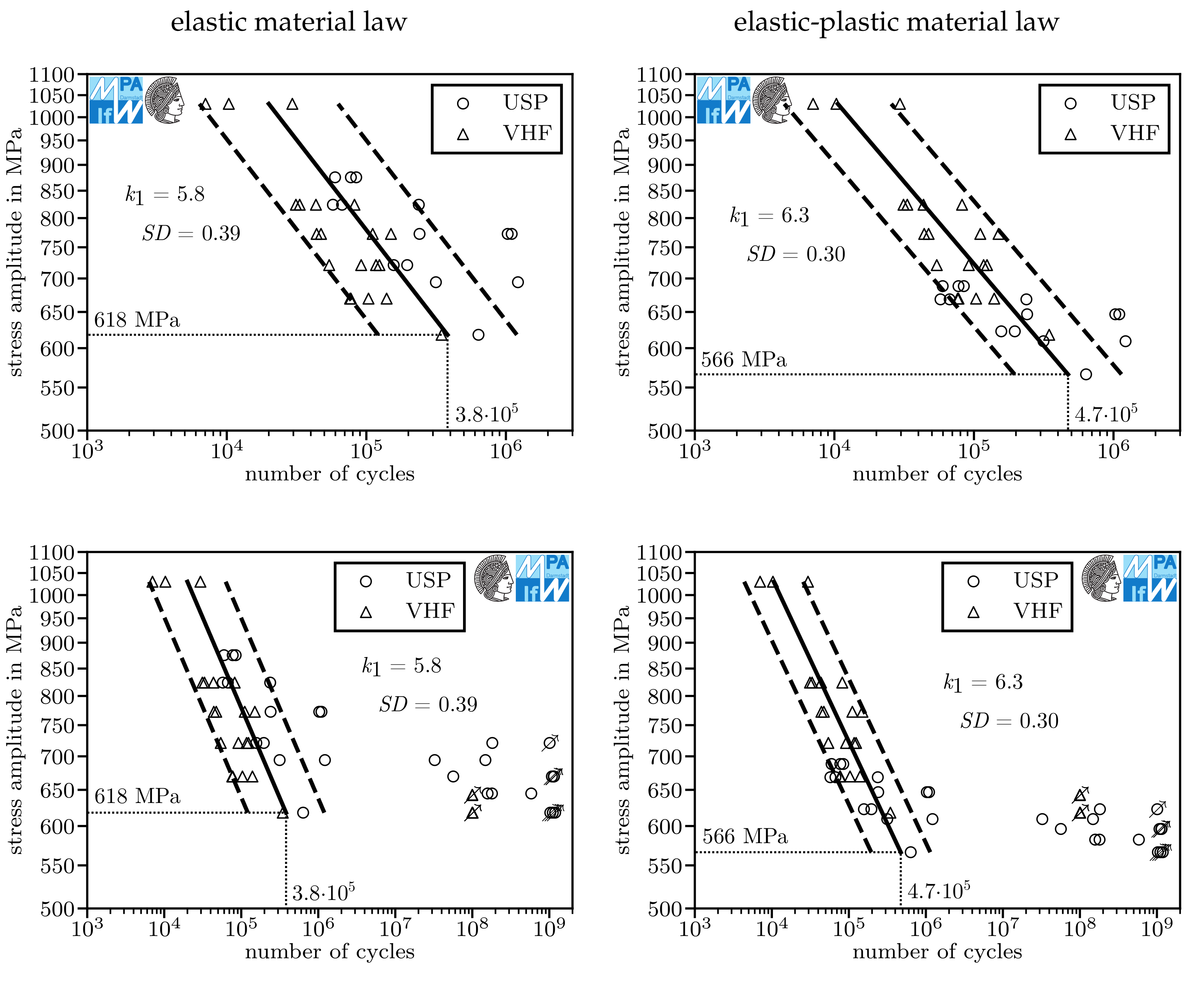
| Figure 11 | 919 MPa | 2.06 | lab air | no | 618 MPa | 3.8×10 | 5.8 | 0.39 | −16.1 | 41 |
| Figure 11 | 919 MPa | 2.06 | lab air | yes | 566 MPa | 4.7×10 | 6.3 | 0.30 | −7.2 | |
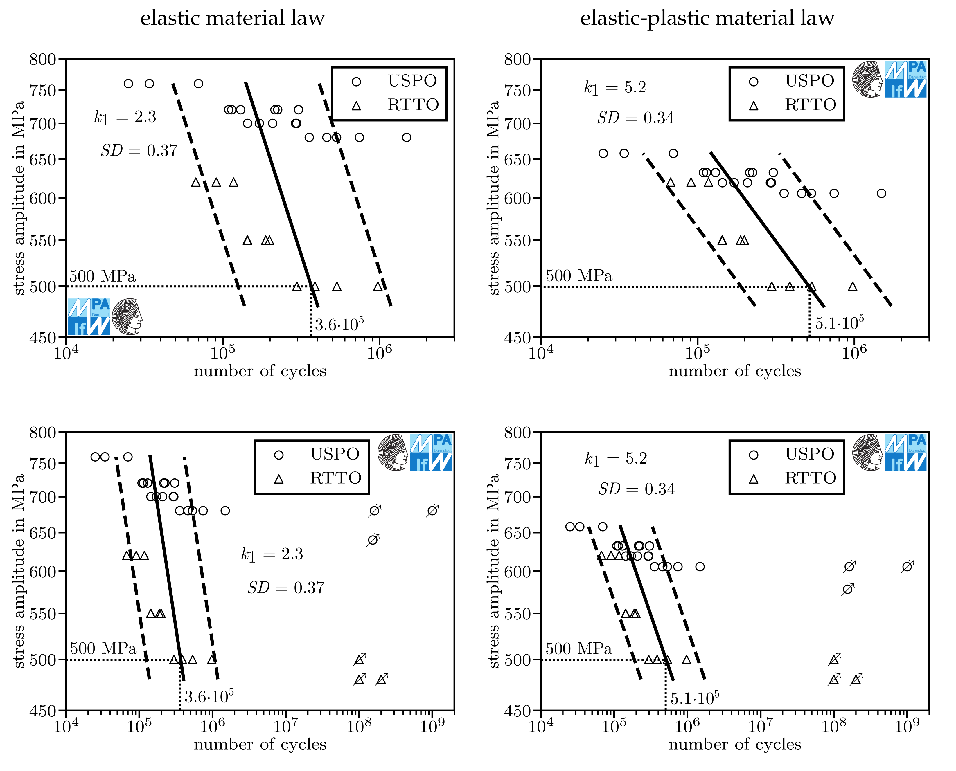
| Figure 12 | 1096 MPa | 1.2 | lab air | no | 500 MPa | 3.6×10 | 2.3 | 0.37 | −12.34 | 30 |
| Figure 12 | 1096 MPa | 1.2 | lab air | yes | 500 MPa | 5.1×10 | 5.2 | 0.34 | −10.2 | |
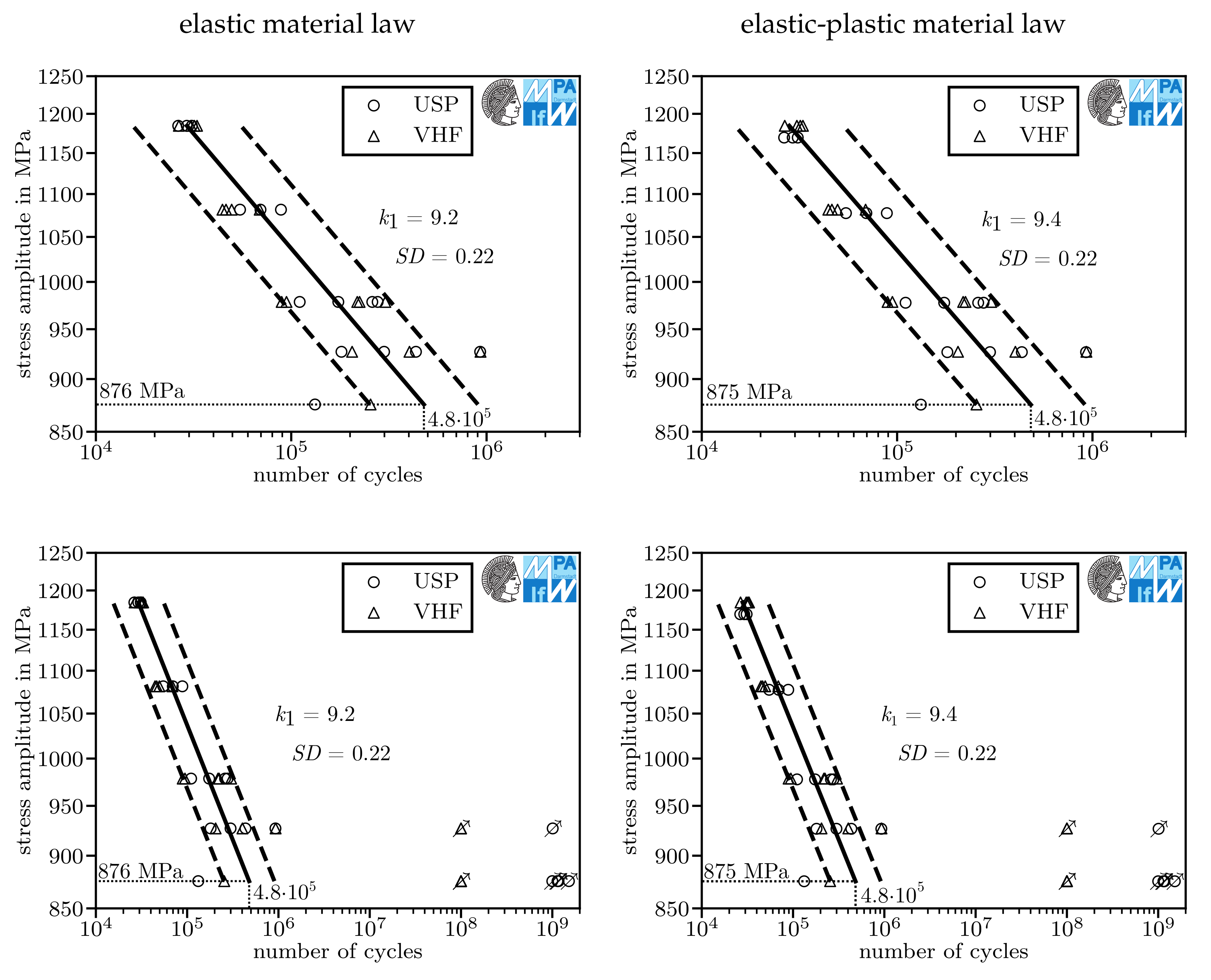
| Figure 13 | 1726 MPa | 2.06 | lab air | no | 876 MPa | 4.8×10 | 9.2 | 0.22 | 3.6 | 32 |
| Figure 13 | 1726 MPa | 2.06 | lab air | yes | 875 MPa | 4.8×10 | 9.4 | 0.22 | 3.6 |
Publisher’s Note: MDPI stays neutral with regard to jurisdictional claims in published maps and institutional affiliations. |
© 2020 by the authors. Licensee MDPI, Basel, Switzerland. This article is an open access article distributed under the terms and conditions of the Creative Commons Attribution (CC BY) license (http://creativecommons.org/licenses/by/4.0/).
Share and Cite
Geilen, M.B.; Schönherr, J.A.; Klein, M.; Leininger, D.S.; Giertler, A.; Krupp, U.; Oechsner, M. On the Influence of Control Type and Strain Rate on the Lifetime of 50CrMo4. Metals 2020, 10, 1458. https://doi.org/10.3390/met10111458
Geilen MB, Schönherr JA, Klein M, Leininger DS, Giertler A, Krupp U, Oechsner M. On the Influence of Control Type and Strain Rate on the Lifetime of 50CrMo4. Metals. 2020; 10(11):1458. https://doi.org/10.3390/met10111458
Chicago/Turabian StyleGeilen, Max Benedikt, Josef Arthur Schönherr, Marcus Klein, Dominik Sebastian Leininger, Alexander Giertler, Ulrich Krupp, and Matthias Oechsner. 2020. "On the Influence of Control Type and Strain Rate on the Lifetime of 50CrMo4" Metals 10, no. 11: 1458. https://doi.org/10.3390/met10111458
APA StyleGeilen, M. B., Schönherr, J. A., Klein, M., Leininger, D. S., Giertler, A., Krupp, U., & Oechsner, M. (2020). On the Influence of Control Type and Strain Rate on the Lifetime of 50CrMo4. Metals, 10(11), 1458. https://doi.org/10.3390/met10111458