Modelling of Fracture Toughness of X80 Pipeline Steels in DTB Transition Region Involving the Effect of Temperature and Crack Growth

Abstract

This work presents an investigation of the effects of temperature and crack growth on cleavage fracture toughness for weld thermal simulated X80 pipeline steels in the ductile-to-brittle transition (DBT) regime. A great bulk of fracture toughness (crack tip opening displacement—CTOD) tests and numerical simulations are carried out by deep-cracked single-edge-notched bending (SENB) and shallow-cracked single-edge-notched tension (SENT) specimens at various temperatures (−90 °C, −60 °C, −30 °C, and 0 °C). Three-dimensional (3D) finite element (FE) models of tested specimens have been employed to obtain computational data. The results show that temperature exerts only a slight effect on the material hardening behavior, which indicates the crack tip constraint (as denoted by Q-parameter) is less dependent on the temperature. The measured CTOD-values give considerable scatter but confirm well-established trends of increasing toughness with increasing temperature and reducing constraint. Crack growth and 3D effect exhibited significant influences on CTOD-CMOD relations at higher temperatures, −30 °C and 0 °C for the SENT specimen.

1. Introduction

Significant effects of crack size and loading mode (bending vs. tension) on fracture toughness values have been revealed from fracture mechanics testing of ferritic structural steels [1]. Previous numerical investigations [2,3] illustrate the strong dependence of crack-tip fields on specimen geometry and remote loading. According to experimental studies by, e.g., Sorem et al., [4] Joyce and Link [5], and others, significant elevations in fracture toughness (characterized as $J_C$ or $K_I{}_C$) for shallow-cracked specimens and/or subjected to tensile loading have been shown. With increasing loads in specific objects, such as a cracked specimen or a structural component, the crack-tip plastic zone is increasingly affected by the nearby traction free boundary according to small-scale yielding (SSY) theory. Due to the crack tip stress relaxation, the constraint level of specimens decreases and further contributes to the apparently increased toughness of shallow-cracked and tension-loaded geometries from fracture mechanics testing [6,7,8]. The stress field surrounding the crack is influenced by the crack tip constraint, which cannot be characterized by single fracture mechanics indicator. The second parameter, such as T-stress [9] or Q-parameter [10,11], has been proposed and developed to further describe the crack-tip stress fields and quantify constraint levels for various geometries and loading modes.

High-strength low-alloyed (HSLA) steels increasingly used for high-pressure pipeline operation and offshore structural installation. The installation of pipelines used for transporting oil and gas sometimes takes place in severe environments, such as in the low-temperature region, where the pipelines must have low-temperature toughness [12]. Thus, the major motivation for the improvement of HSLA steels has been provided by the demands for higher strength as well as improved toughness, ductility, and weldability at low temperatures [13,14]. Though the HSLA steels own the excellent properties of tensile strength and ductile to brittle transition (DBT), according to the Charpy-impact test investigation, the ductile brittle transition (DBT) on the basis of microscopic mechanism occurs with decreases of temperature. On the other hand, X80 steel pipelines are exposed in extreme low-temperature environments, and it is meaningful to characterize the fracture toughness with temperature variations during the processing of DBT. The balance of high strength and toughness can be deteriorated by welding thermal cycles, producing local poor toughness in the welded joints [15]. The heat-affected zone (HAZ) of a weldment is in many cases considered to be the weakest part and is crucial in the failure of steel structures because of its heterogeneous microstructure produced during the welding process [16,17]. Therefore, treatment of brittle fracture in weldment and HAZ is challenging. In the 1990s, there was a significant focus on characterizing the local stress fields in weldment and HAZ. SINTEF/NTNU developed the so-called J-Q-M theory (see, e.g., Zhang et al. [18,19,20]) where both constraint effects due to geometry and material mismatch were included in characterization of the local stress field ahead of the crack tip. In addition, some researchers have investigated the related HAZ properties of high-strength steels on the basis of physical simulation, welding heat input effect on HAZ in S960QL steel, and the matching effect on fatigue crack growth behavior of high-strength steels GMA welded joints [21,22,23,24].

This paper mainly focuses on the single-edge-notched tension (SENT) and single-edge-notched bending (SENB) specimens, which are usually used to characterize pipeline steels with thin-walled thickness, as specified recently by a so-called SENT methodology to identify a SENT specimen(s) to match the crack tip constraint of cracked pipe sections. The effect of constraint on the fracture toughness of weld thermal simulated X80 pipeline steels in the ductile-to-brittle transition relationship is clarified by combination of experimental assessment and numerical simulation. The fracture toughness comparison of X80 steel SENB specimens (a/W = 0.5) under different temperature have been presented in [25]. The material is determined by the increasing demand due to a great account of applications for manufacturing high-strength pipes for the oil and gas industry. Fracture toughness (as denoted by crack tip opening displacement (CTOD)) tests are performed at different temperatures, −90 °C, −60 °C, −30 °C, and 0 °C. Both the traditionally used deeply cracked SENB specimens with a/W = 0.5 and SENT specimens with a/W = 0.3 are used to characterize the crack tip constraint effect on the fracture toughness in the ductile-to-brittle transition region. 3D nonlinear finite element models are employed to analyze the crack-tip stress fields of tested specimens by considering the effects of the constraint and without/with crack growth on fracture toughness. The numerical analysis is compared with the experimental results.

2. Experimental Details

2.1. Material Description

The material used in our study is the HSLA X80-grade steel, which has a minimum yield strength of 555 MPa (tensile strength 625 MPa). The nominal outer diameter of the pipe is 510 mm, and the nominal wall thickness is 14.6 mm. The typical chemical composition of this material is listed in

Table 1. Chemical composition of the X80 steel (wt. %).

Steel	C	Si	Mn	P	S	Others
X80	0.04~0.07	~0.25	≤1.8	≤0.01	≤0.001	Mo, Ni, Cu, Ti, Nb, V, Al

.

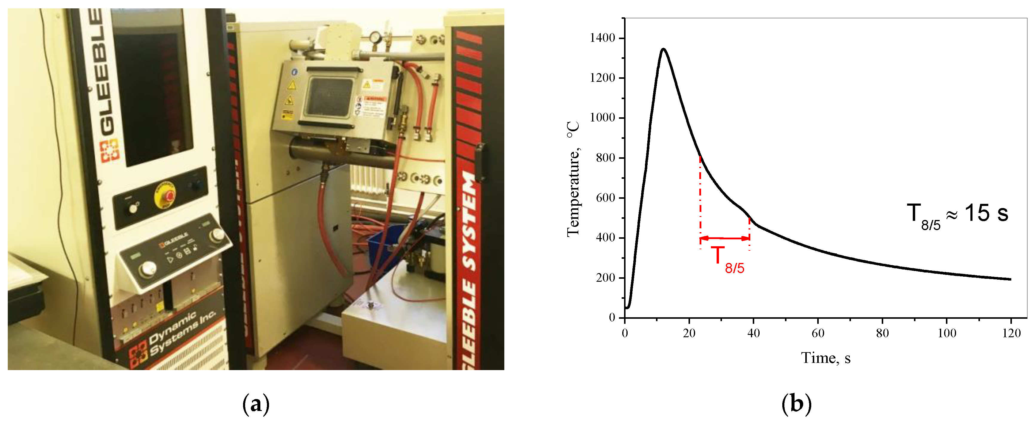
2.2. Weld Thermal Simulation Technique

The weld thermal simulation technique is used to obtain the tested specimens. The single welding cycle simulation is intended to represent the coarse-grained HAZ (CGHAZ) of the welds [26], which has been used in the preparation of weld thermally simulated specimens. In this study, the specimens were heated to the maximum temperature of 1350 °C by resistance-heating in a computer-controlled Gleeble weld thermal simulator (Figure 1a). The whole temperature vs. time history applied during the weld thermal simulation can be seen in Figure 1b. The thermal history is described as a sequence of heating and cooling intervals. The simulation was performed by heating the sample to 1350 °C for 2 s followed by controlled cooling; the cooling intervals were 2 s in the 1350 °C–1200 °C range, and 15 s between 800 °C–500 °C. Thus, the T8/5 is 15 s. The synthetic CGHAZ microstructure was thereafter produced in a certain region in the specimen where the fatigue pre-crack is introduced after being machined. The prior austenite grain size of CGHAZ was measured to be about 50 µm.

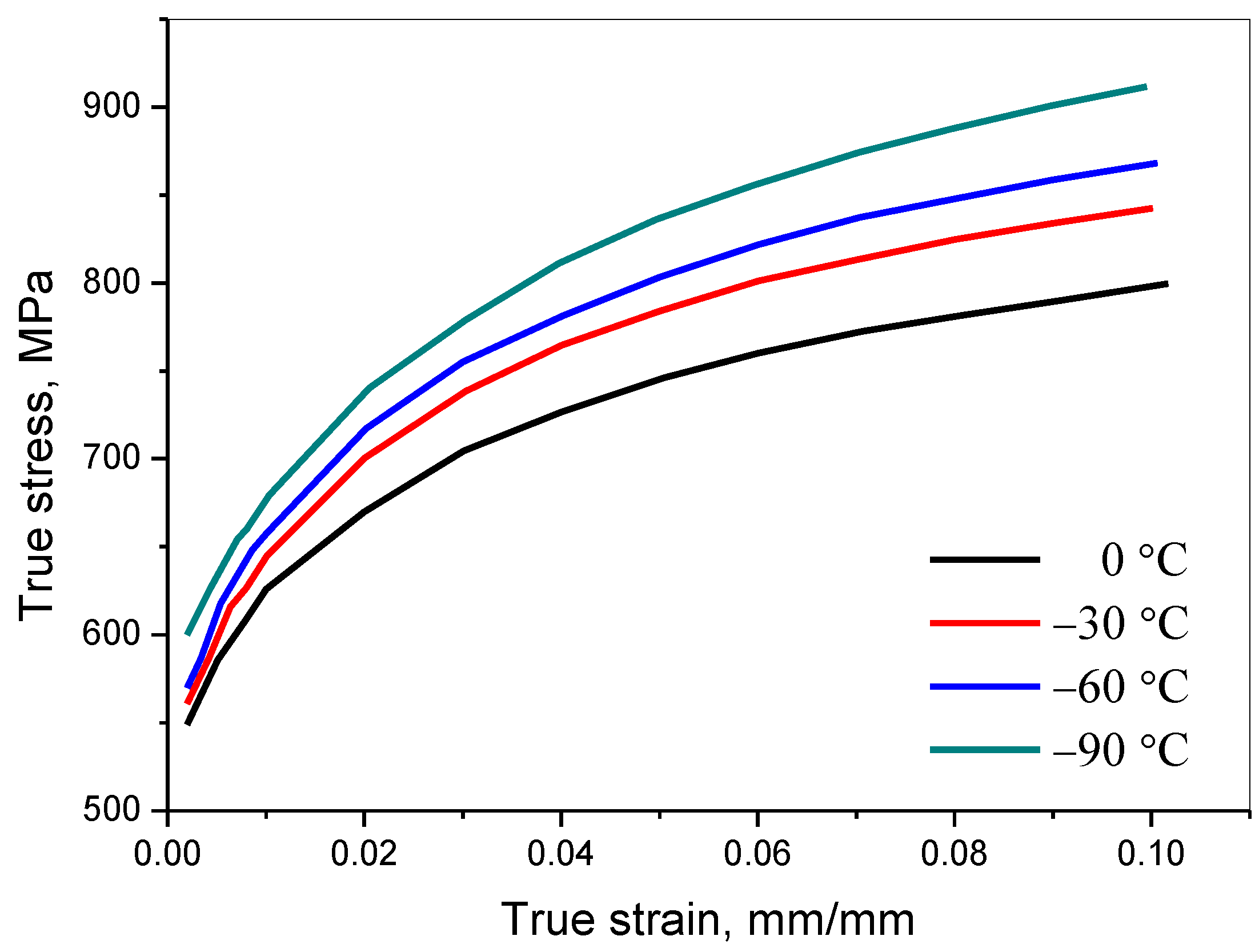
2.3. The True Stress-Strain Curves

To characterize the material flow properties in 3D finite element model, the true stress-strain curves of material (CGHAZ in X80) were measured by smooth round bar tensile tests at four temperatures as shown in Figure 2. The results show that yield strength here slightly increases with decreasing temperatures. There is also a weak trend of increasing work hardening with decreasing temperatures.

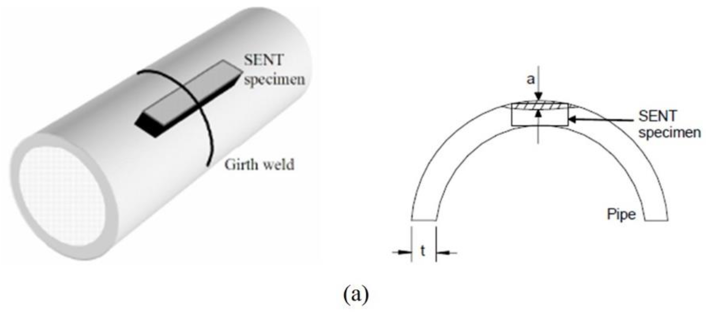
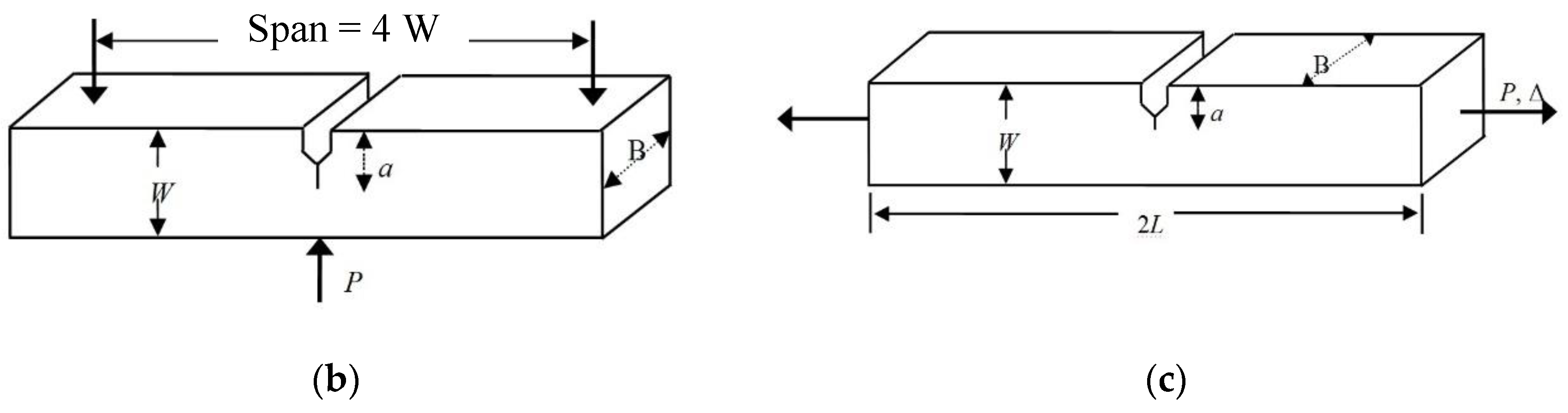
2.4. Specimen Configurations and Test Program

The geometrical configurations are schematically drawn in Figure 3 for SENB and SENT specimens, which are directly extracted from the X80 pipeline with specimen length along the pipeline longitudinal direction and crack propagation following the pipe thickness orientation, as shown in Figure 3a. For all specimens, a thickness of B = 10 mm and width of W = 10 mm with crack length (denoted by a), to width ratio of a/W = 0.5 for SENB and a/W = 0.3 for SENT specimens have been considered. The span of the specimen, S, is chosen to be four times of width, W, for SENB (S/W = 4) and L/W = 3 for SENT.

The SENB specimens are prepared and tested according to the standard of BS 7448 [27], while the SENT fracture specimens are machined in accordance with the “Recommended Practice DNV-RP-F108” [28]. Double clip gauge was used to digitally record the load-CMOD (crack mouth opening displacement) curves during the tests. The CTOD values are determined at the maximum load through measured load-CMOD records. The tensile and bending tests were performed at four different temperatures, −90 °C, −60 °C, −30 °C, and 0 °C. The testing rate is 0.5 mm/min of crosshead displacement for each specimen. For each specimen geometry, 10 parallel tests have been carried out at each temperature. After each test, the fatigue pre-cracking length and ductile crack extension that occurred during the test were measured using an optical microscope. The notches were located in the center of the weld, as can be seen in Figure 3.

3. Numerical Procedures

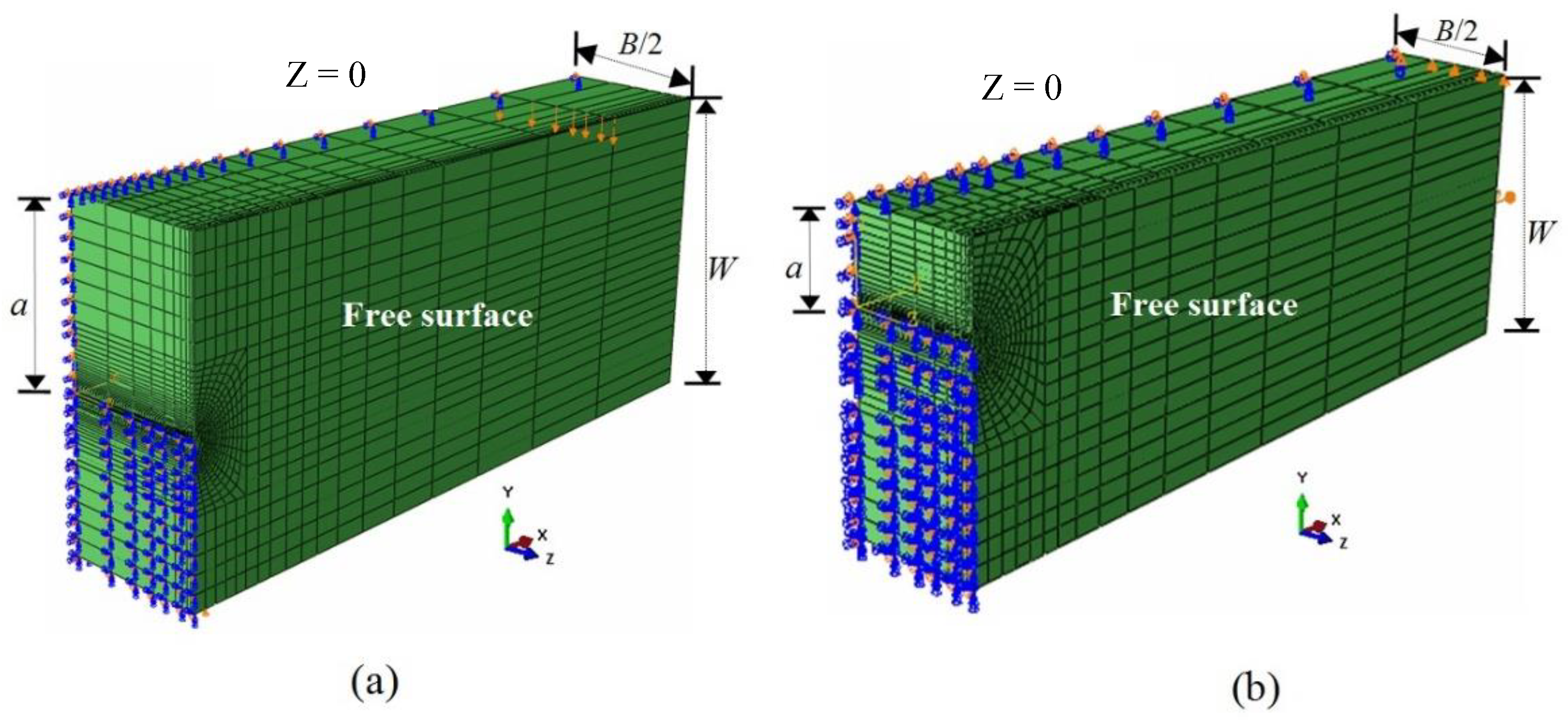
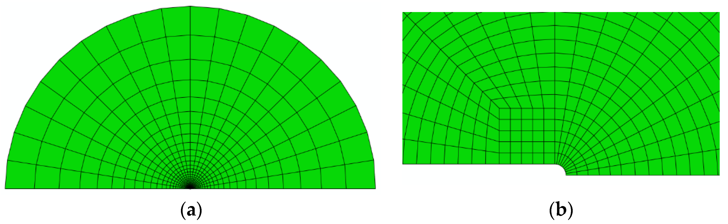
3.1. 3D Finite Element Models

3D finite element models were built using ABAQUS [29] for SENB and SENT specimens as shown in Figure 4. Due to symmetry, one-quarter of the specimen is modeled for finite element analysis considering the geometrical symmetry. A typical mesh configuration of elements surrounding the crack front is used with a small notch (with a notch root radius of r = 2 μm) in front of the crack tip. A 3D continuum element with eight-node, full integration (ABAQUS: C3D8), is used for FE calculations. The X80 steel true stress-strain curves obtained from the smooth round bar tensile tests at corresponding temperatures are applied for 3D model calculations. Meanwhile, the nonlinear geometric effect (NLG) is considered in all the finite element analyses. The CTOD-value is extracted from the displacement of a node in front of the initial crack tip [30].

3.2. The MBL (Modified Boundary Layer) Model

In calculating the Q-parameter (quantitative characterization of crack tip constraint), the MBL model solution with T = 0 (here, T is the elastic T-stress, which is defined as constant stress acting parallel to the crack and its magnitude is proportional to the nominal stress in the vicinity of the crack) is adopted herein to represent the reference stress field for each case. Due to symmetry, only one-half of the model has been used in the MBL model, as shown in Figure 5. The global finite element mesh for the MBL model is drawn in Figure 5a. Similar models have been used in other studies [31,32,33]. Details of the mesh in the local region of the crack tip can be seen in Figure 5b. The MBL is a plane strain model with the same mesh arrangement in front of the crack tip (with a notch root radius of r = 2 µm) as in 3D models.

4. Results and Discussion

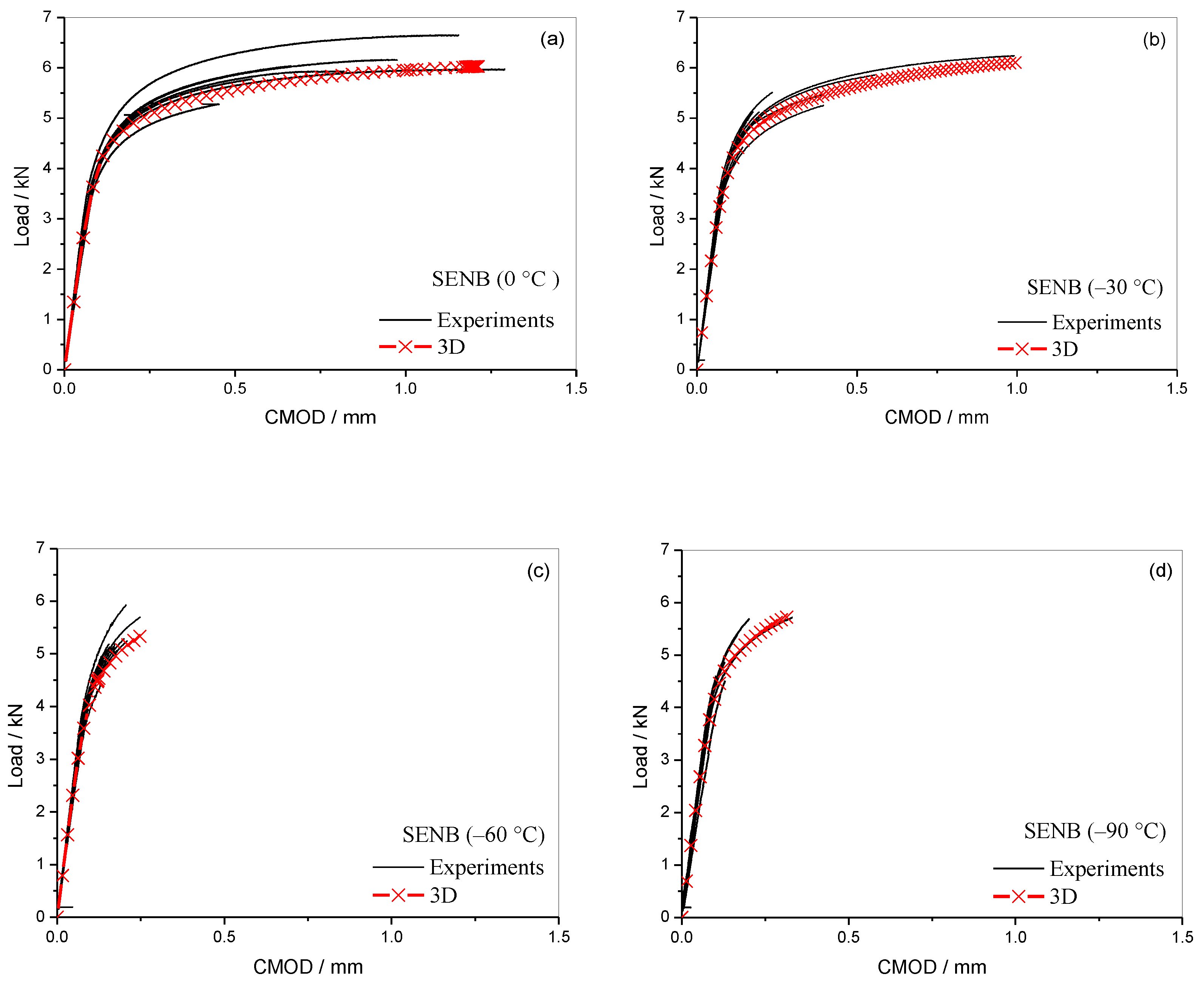
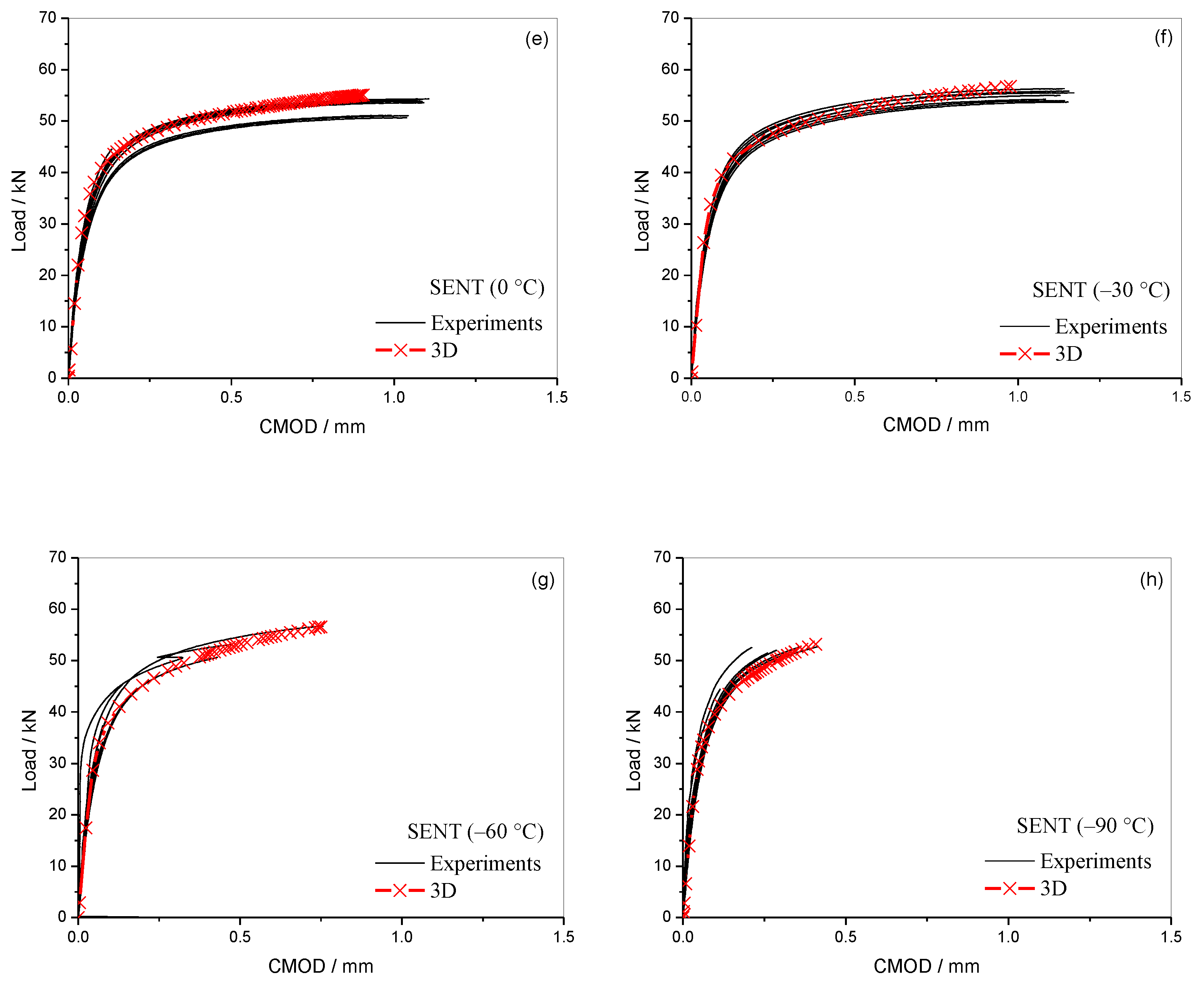
4.1. Measured and Calculated Load-CMOD Curves

The measured and calculated load-CMOD curves for all specimens at various temperatures are plotted in Figure 6. Only mid-thickness values of CMODs are extracted through the specimen thickness for all cases in this subsection. It can be seen that numerical simulations of load-CMOD curves are in good accord with experimental results for all temperatures. The material becomes quite brittle, which can be clearly seen from the flat fracture surface, and no significant crack growth has been observed from optical microscope observations for both the SENB and SENT specimens at lower temperatures, for example −90 °C and −60 °C. For the SENB specimens at −30 °C and 0 °C, small subcritical (mostly less than 0.2 mm) crack growth has been observed; whereas evident crack growth ($\Delta a$ > 0.2 mm) have been observed for the SENT specimens at −30 °C and 0 °C. For the sake of simplicity, no crack growth has been considered in the 3D models in this subsection.

According to test demands of SENT and SENB specimen, 10 parallel tests have been carried out at each temperature. In addition, it can be argued that the transferability of the true $\sigma -\epsilon$ curve from round thermal simulated tensile bar to the fracture mechanics specimens is quiet well. One thing that should be noted is that the average crack depth for both the SENB and SENT specimens at each temperature is used in these 3D models.

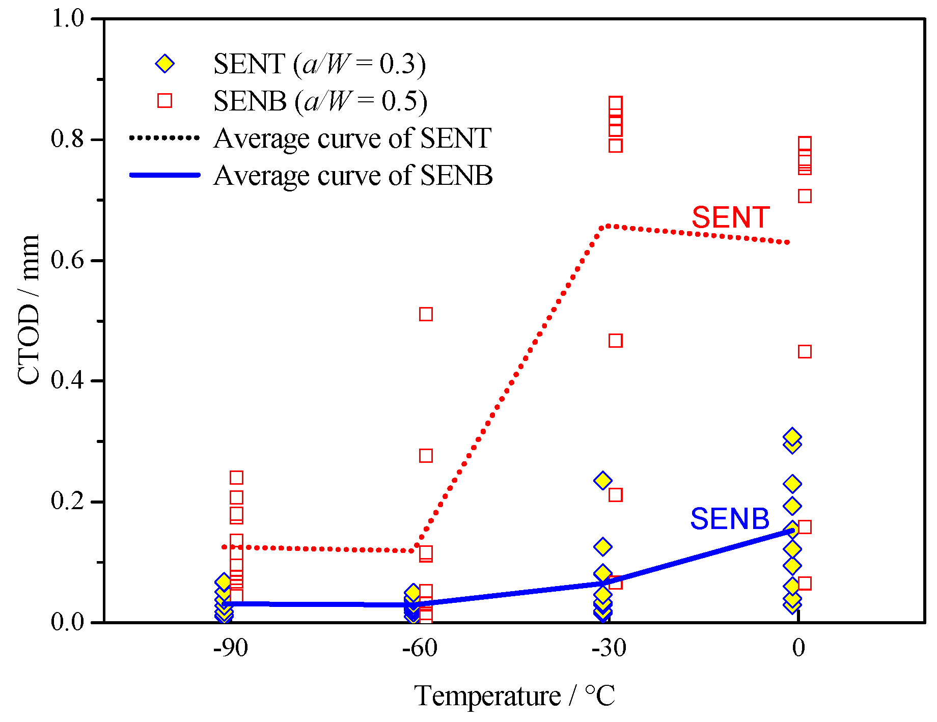
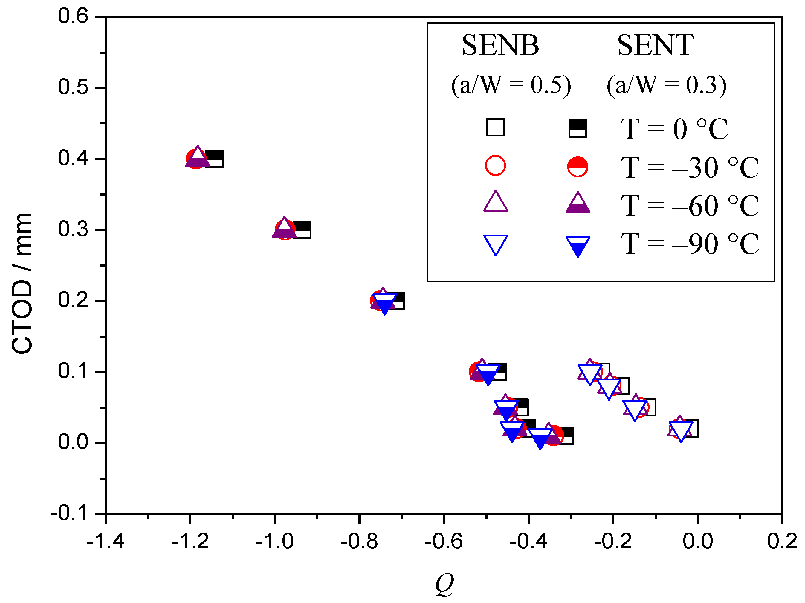
4.2. Measured CTOD-Values and Calculated Q-CTOD Relations at Different Temperatures

The results of fracture toughness (CTOD-value) as a function of temperature and their related average curves for SENT and SENB specimens are presented in Figure 7. It shows that the average CTOD values of SENT specimens at each temperature are obviously higher than that of SENB specimens. To illustrate the scatter degree of fracture toughness test data in Figure 7, the statistical characteristics are conducted quantitatively. The related analysis results for SENB and SENT specimens are summarized in

Table 2. Statistical characteristics of test data for SENB and SENT specimens.

Specimens	Statistical Characteristics	−90 °C	−60 °C	−30 °C	0 °C
SENB	Average values (mm)	0.031	0.029	0.065	0.152
	Standard deviation	0.021	0.011	0.064	0.096
	Standard deviation coefficient	0.703	0.392	0.979	0.632
SENT	Average values (mm)	0.125	0.119	0.658	0.63
	Standard deviation	0.055	0.151	0.284	0.098
	Standard deviation coefficient	0.439	1.274	0.432	0.155

. According to the average CTOD variations in statistical characteristics, these data increase with the temperature elevation from −90 °C to 0 °C for these two specimen types. In addition, from the perspective of standards variation coefficient, it stands for the ratio of the standard deviation to the mean. The higher the coefficient of variation, the greater the level of dispersion around the mean. It can be seen from Table 2 that the dispersion of −30 °C test data is the largest for SENB specimens, and −60 °C test data dispersion is the largest for SENT specimens. Thus, a definite temperature-dependence on dispersion characteristic cannot be drawn from these test data.

It shows that the fracture toughness tends to be scattered at each temperature. Also, the scatter of fracture toughness increases rapidly with increasing temperatures (upper transition region), for instance −30 °C and 0 °C, where a ductile mechanism is involved and cleavage instability may intervene after a certain amount of ductile crack growth as have been observed from the tests, especially for SENT specimens.

Additionally, the average fracture toughness values are higher for SENT specimens with a shorter crack of a/W = 0.3 compared to the SENB specimens with a/W = 0.5 at each test temperature. Moreover, this difference becomes larger with increasing temperatures.

The detailed effects of temperature and specimen geometry (as quantitatively characterized by crack tip constraint—Q-parameter) on fracture toughness will be studied in the following. As has been known, the J-Q methodology gives a direct measurement of the crack-tip stress field of interest that is related to a reference field [10,11], and can therefore describe the evolution of constraint ahead of the crack tip throughout the loading to large-scale yielding (LSY), where J sets the deformation level and Q is a stress triaxiality parameter. In this paper, the Q-parameter has been used to quantify the crack tip constraint for each specimen at each temperature.

The Q-parameter was originally defined as follows [10],

$$Q=\frac{{\sigma }_{\theta \theta }-{({\sigma }_{\theta \theta }{}^{\mathrm{Re}f})}_{T=0}}{{\sigma }_0}, x/(J/{\sigma }_0)=2, \theta =0.$$

(1)

where ${\sigma }_{\theta \theta }$ is the opening stress component of interest, $({\sigma }_{\theta \theta }{}^{\mathit{Ref}}{)}_{T=0}$ is the reference stress component characterized by MBL model solution with T = 0, ${\sigma }_0$ is the yield stress, and x denotes the distance from the crack tip along the crack plane (θ = 0).

CTOD is selected as the crack driving force in our stud; the following constrain effect definition of Q has been used [27,28]:

$$Q=\frac{{\sigma }_{\theta \theta }{}^{specimen}-{({\sigma }_{\theta \theta }{}^{\mathrm{Re}f})}_{T=0}}{{\sigma }_0},\mathrm{at}\mathrm{x}/\mathrm{CTOD}=4,\theta =0.$$

(2)

where ${\sigma }_{\theta \theta }{}^{specimen}$ is the opening stress component of the specimen at a certain temperature, $({\sigma }_{\theta \theta }{}^{\mathit{Ref}}{)}_{T=0}$ is the reference stress component at the same temperature, and other parameters are the same as defined in Equation (1). Only the distribution of the crack tip opening stress (${\sigma }_{22}$ at $\theta =0$) has been studied. In the following, the results of crack tip opening stress distribution at different CTODs are presented in Figure 8 for specimens at 0 °C.

For SENT specimen as shown in Figure 8b, it demonstrates that the opening stress distribution in front of the crack tip is nearly parallel to the reference stress field. However, global bending causes the slope of the opening stress distribution to gradually deviate from the reference field for SENB specimen, but still remainsquite similar, as can be seen in Figure 8a. Similar observations have also been found for specimens at other temperatures while the results are not included herein for the sake of simplicity.

The calculated Q-CTODs relations are displayed in Figure 9 for SENB and SENT specimens at various temperatures. Only the mid-thickness layer was used to compute Q-parameter herein. The Q-parameter stands for constraint effect decreases with the increases of CTODs. Meanwhile, the Q-parameter for SENB specimen for each temperature level is considerably larger than that of SENT at same CTODs, which means the crack tip constraint of SENB specimen is higher than that of SENT as has been observed. Nearly constant Q-parameters have been computed for all temperatures considered at the same CTOD values. The results present a weak dependence of temperature on the constraint ahead of the crack tip that can be expected for SENT specimen compared with that of SENB specimen.

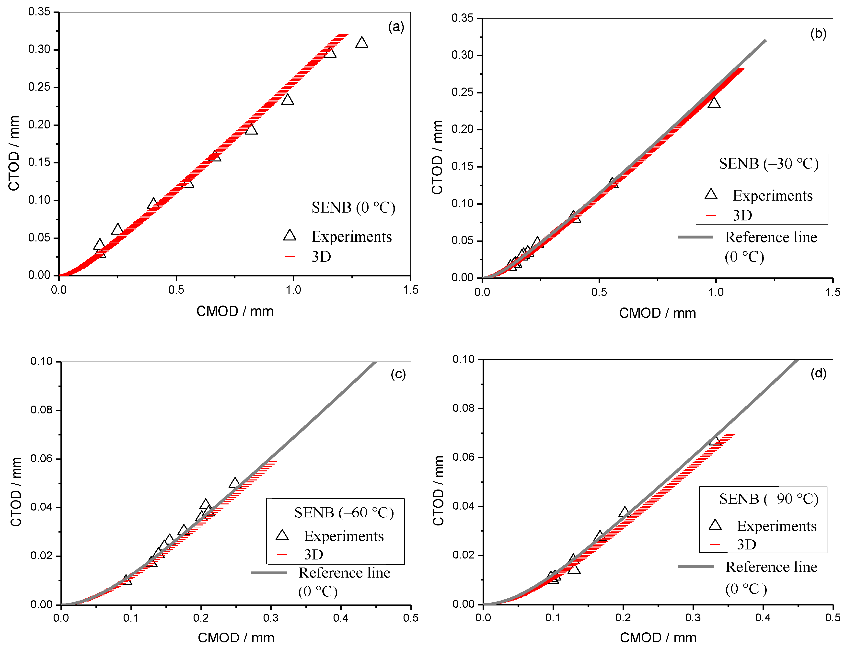
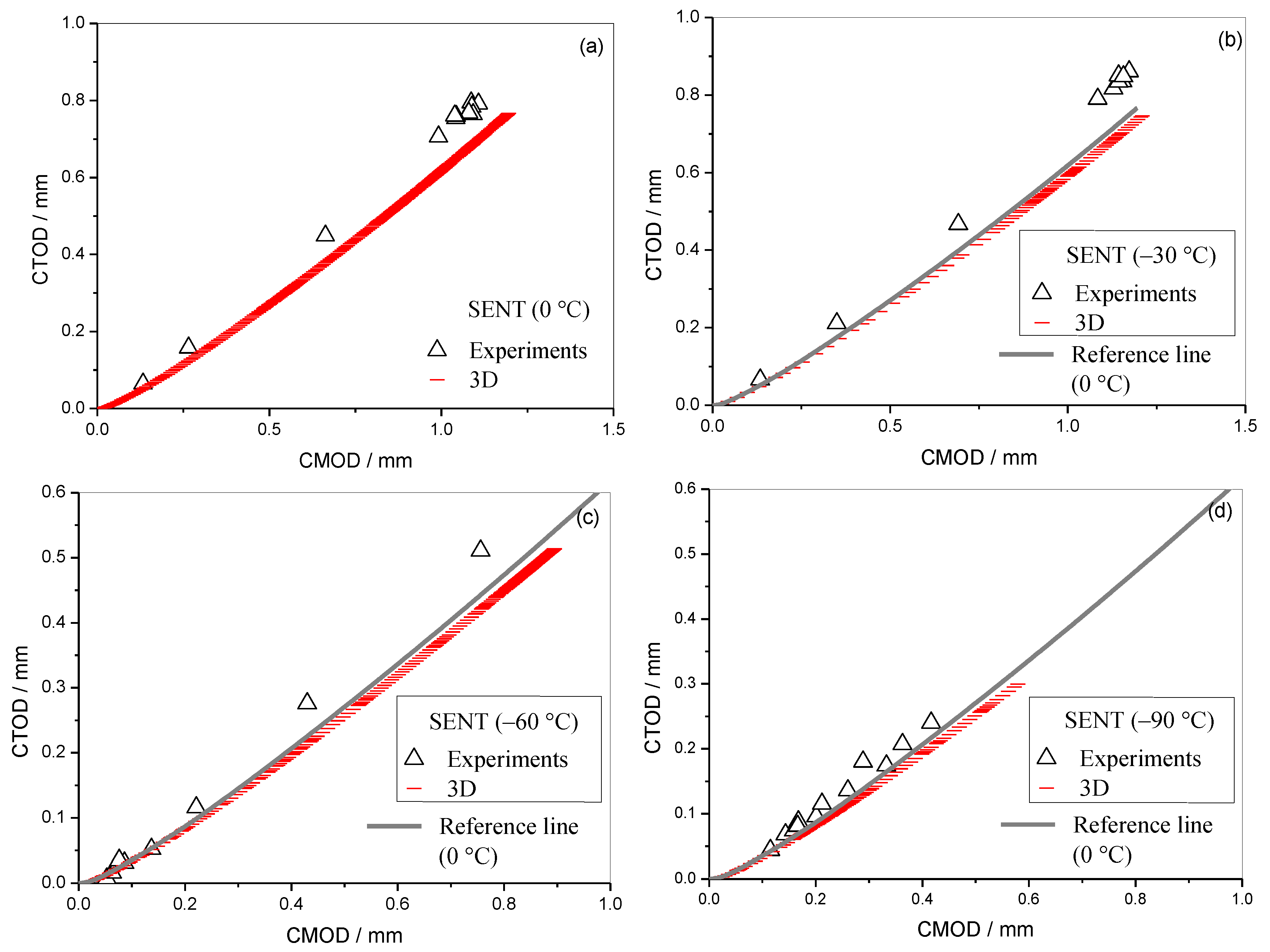
4.3. Measured and Calculated CTOD-CMOD Relations

As has been shown in Section 4.1, the experimental results are in good accordance with numerical simulations for the load-CMOD curves for all specimens at each temperature; how the 3D finite element models work for predicting the local fracture parameter as denoted by CTOD will be discussed in this subsection.

Figure 10 and Figure 11 draws the CTODs vs. CMODs relationship obtained from both experiments and numerical calculations for all specimens at various temperatures without considering crack growth. Still, only mid-thickness values of CTODs versus CMODs are extracted herein. It can be seen that the tested results of CTOD-CMOD relations for the SENB specimens (Figure 10) can be quite well predicted by 3D FEA results at all temperatures.

As for the SENT specimens (Figure 11), a certain difference between experiments and 3D FE simulations can be observed at all temperatures. For small CTODs (less than 0.2 mm), quite good accordance can be obtained between experiments and simulations for all temperatures. However, the predicted CTOD values from the 3D models start to deviate from experimental results with the increases of CTODs, especially for the cases at higher temperatures, 0 °C and −30 °C. This is a remaining issue and more efforts are needed in further work, for example, the influences of local inhomogeneity of microstructure in HAZ and ductile crack propagation can be considered to further modify the models so as to improve the validity and accuracy of simulations with respect to the experiments. In this respect, it is noted that no standard for CTOD measurements in SENT specimens currently exists. The results in this paper warrant the need for further work in order to arrive at a method for experimental measurements of CTOD in SENT specimens, which could eventually form the basis for a standard document.

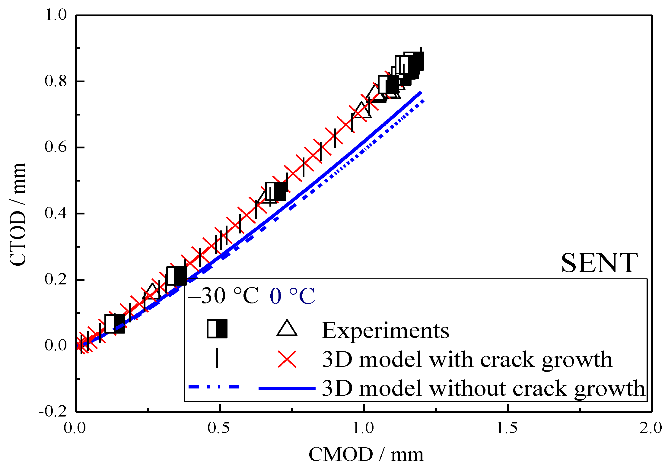
4.4. The Effect of Crack Growth on the CTOD-CMOD Relations

In this subsection, the effect of crack growth on CTOD-CMOD relations for the SENT specimen at 0 °C and −30 °C are considered in 3D models. Only mid-thickness values for both the CTODs and the CMODs are plotted in Figure 12. The complete Gurson model (see Reference [34]) is involved in calculating crack growth in 3D models. It can be seen that a significant elevation in fracture toughness for SENT specimens by considering crack growth. Also, a wonderful agreement between experiments and 3D FE simulations can be achieved by considering the influence of crack growth on fracture toughness for SENT specimens at both 0 °C and −30 °C. It can be concluded that the ductile crack extension is dependent on the temperature. In the low temperature range, it almost occurs at the cleavage fracture. The ductile crack extension mechanism involved in the upper transition zone of DBT, which cannot be ignored to predict CTOD-value for pipeline steel integrity assessment.

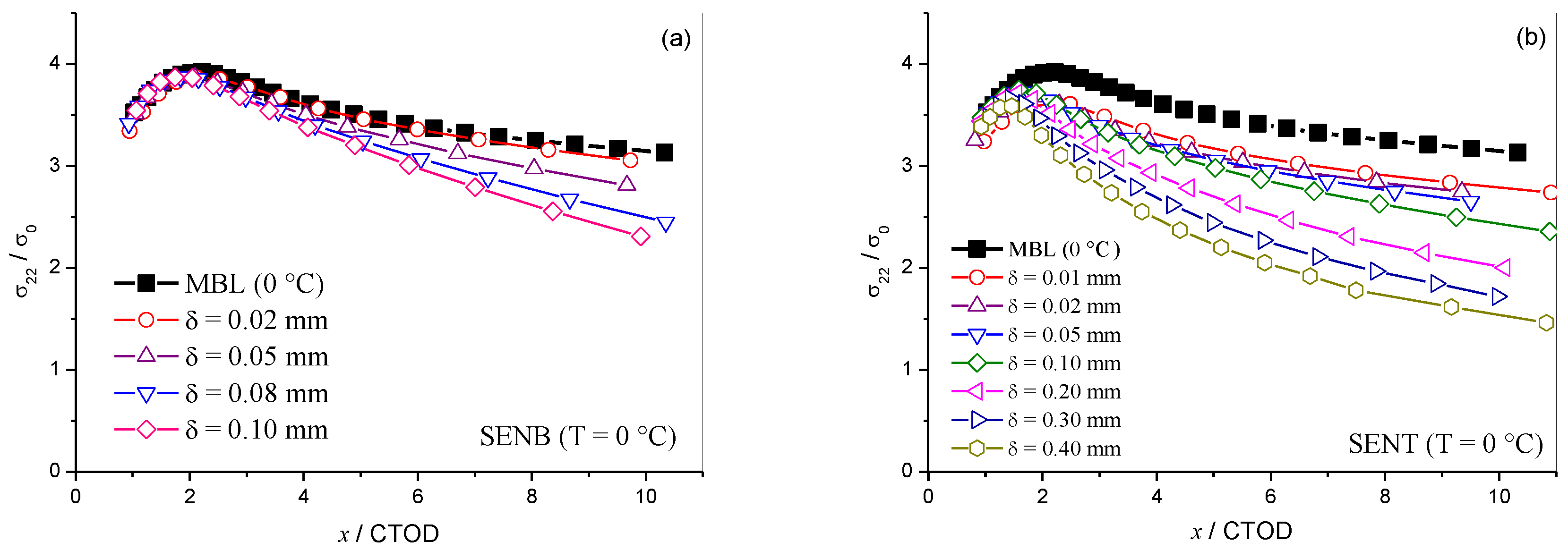
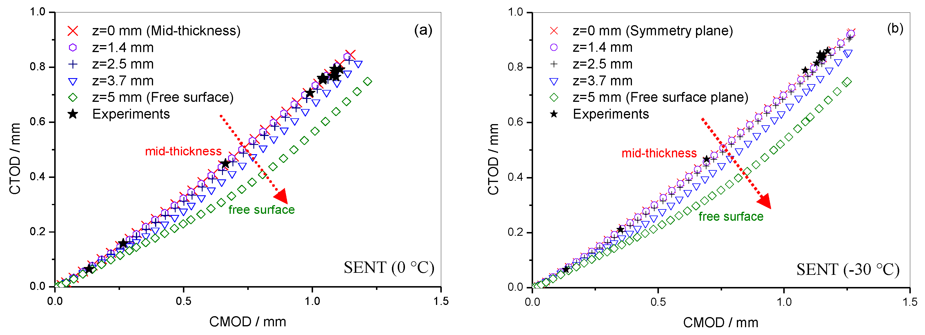
4.5. The Influence of 3D Effect on the Fracture Toughness

In order to find the influence of 3D effect on fracture toughness, the calculated CTOD-CMOD relations at different layers through the specimen thickness compared with experiments are displayed in Figure 13. Two cases of SENT specimens considering crack growth at 0 °C and −30 °C are selected for this question. It can be seen that CTOD-CMOD values change considerably through the specimen thickness. The greater the distance from the specimen mid-thickness, the greater the deviation from experiments. In addition, the predicted CTOD-CMOD relations near the mid-thickness layer are coincident well with the experiments.

5. Conclusions

In this paper, the HAZ of X80 high-strength steel is studied by experimental and simulation methods. The following conclusion can be drawn as follows:

(1)

The HAZ of X80 hardening behavior exhibits a slight effect of temperature variations, which indicates the crack tip constraint is less dependent on the temperature as also observed from 3D FEA results.

(2)

The predicted load-CMOD curves from 3D models are in good accordance with experimental results at all temperatures. As for the local fracture parameter, as depicted with the CTOD-CMOD relationship, the experimental data for the SENB specimens can be quite well simulated by 3D simulations without considering crack growth. For the SENT specimens, a good agreement between experiments and numerical simulations can also be obtained by considering the effect of crack growth in the 3D models.

(3)

The tested CTOD-values show considerable scatter but confirm well-established trends of increasing toughness with increasing temperature and reducing constraint.

(4)

Cleavage fracture can be clearly observed for SENB specimens at all tested temperatures, while ductile crack growth can be seen for SENT specimens at −30 °C and 0 °C.

(5)

From 3D finite element analyses, it has been found out that the CTODs change considerably through the specimen thickness. The predicted CTODs near the mid-thickness layer is coincident well with the experiments for the SENT specimens at 0 °C and −30 °C. The greater the distance from the specimen mid-thickness, the greater the deviation from experiments.

References

1. Mathias, L.L.; Sarzosa, D.F.; Ruggieri, C. Effects of specimen geometry and loading mode on crack growth resistance curves of a high-strength pipeline girth weld. Int. J. Press. Vessels Pip. 2013, 110, 12–22. [Google Scholar] [CrossRef]
2. McMeeking, R.M.; Parks, D.M. On Criteria for J-Dominance of Crack-Tip Fields in Large-Scale Yielding. In ASTM STP 668 Elastic-Plastic Fracture; Landes, J.D., Ed.; ASTM International: Philadelphia, PA, USA, 1979; pp. 175–194. [Google Scholar]
3. Shih, C.F.; German, M.D. Requirements for a one parameter characterization of crack-tip fields by the HRR singularity. Int. J. Fract. 1981, 17, 27–43. [Google Scholar]
4. Sorem, W.A.; Dodds, R.H.; Rolfe, S.T. Effects of crack depth on elastic-plastic fracture toughness. Int. J. Fract. 1991, 47, 105–126. [Google Scholar] [CrossRef]
5. Joyce, J.A.; Link, R.E. Ductile-to-brittle transition characterization using surface crack specimens loaded in combined tension and bending. In ASTM STP 1321 Fatigue and Fracture Mechanics; Underwood, J.H., Macdonald, B., Mitchell, M., Eds.; ASTM International: Philadelphia, PA, USA, 1997; Volume 28, pp. 243–262. [Google Scholar]
6. Dodds, R.H., Jr.; Shih, C.F.; Anderson, T.L. Continuum and micromechanics treatment of constraint in fracture. Int. J. Fract. 1993, 64, 101–133. [Google Scholar]
7. Dodds, R.H., Jr.; Nevalainen, M. Numerical investigation of 3-D constraint effects on brittle fracture in SE (B) and C (T) specimens. Int. J. Fract. 1996, 74, 131–161. [Google Scholar]
8. Naumenko, V.P.; Limanskii, I.V. Fracture resistance of sheet metals and thin-wall structures. Part 1. critical review. Strength Mater. 2014, 46, 18–37. [Google Scholar] [CrossRef]
9. Betegon, C.; Hancock, J.W. Two-parameter characterization of elastic-plastic crack-tip fields. J. Appl. Mech. 1991, 58, 104–110. [Google Scholar] [CrossRef]
10. O’Dowd, N.P.; Shih, C.F. Family of crack-tip fields characterized by a triaxiality parameter-I. Structure of fields. J. Mech. Phys. Solids 1991, 39, 989–1015. [Google Scholar] [CrossRef]
11. O’Dowd, N.P.; Shih, C.F. Family of crack-tip fields characterized by a triaxiality parameter-II. Fracture application. J. Mech. Phys. Solids 1991, 40, 939–963. [Google Scholar] [CrossRef]
12. Bose-Filho, W.W.; Carvalho, A.L.M.; Stragwood, M. Effects of alloying elements on the microstructure and inclusion formation in HSLA multipass welds. Mater. Charact. 2007, 58, 29–39. [Google Scholar] [CrossRef]
13. Das, S.K.; Sivaprasad, S.; Das, S.; Chatterjee, S.; Tarafder, S. The effect of variation of microstructure on fracture mechanics parameters of HSLA-100 steel. Mater. Sci. Eng. A 2006, 431, 68–79. [Google Scholar] [CrossRef]
14. Bose Filho, W.W.; Carvalho, A.L.M.; Bowen, P. Micromechanisms of cleavage fracture initiation from inclusion in ferritic welds: Part, I. Quantification of local fracture behavior observed in notched test pieces. Mater. Sci. Eng. A 2007, 460–461, 436–452. [Google Scholar] [CrossRef]
15. Lambert-Perlade, A.; Gourgues, A.F.; Besson, J.; Sturel, T.; Pineau, A. Mechanisms and modeling of cleavage fracture in simulated heat-affected zone microstructures of a high-strength low alloy steel. Metall. Mater. Trans. A 2004, 35, 1039–1053. [Google Scholar] [CrossRef]
16. Mohseni, P.; Solberg, J.K.; Karlsen, M.; Akselsen, O.M.; Østby, E. Investigation of mechanism of cleavage fracture initiation in intercritically coarse grained heat affected zone of HSLA steel. Mater. Sci. Technol. 2012, 28, 1261–1268. [Google Scholar] [CrossRef] [Green Version]
17. Moeinifar, S.; Kokabi, A.H.; Hosseini, H.R.M. Influence of peak temperature during simulation and real thermal cycles on microstructure and fracture properties of the reheated zones. Mater. Des. 2010, 31, 2948–2955. [Google Scholar] [CrossRef]
18. Zhang, Z.L.; Hauge, M.; Thaulow, C. Two-parameter characterization of near-tip stress fields for a bi-material elastic-plastic crack. Int. J. Fract. 1996, 79, 65–83. [Google Scholar] [CrossRef]
19. Thaulow, C.; Hauge, M.; Zhang, Z.L.; Ranestad, O.; Fattorini, F. On the interrelationship between fracture toughness and material mismatch for cracks located at the fusion line of weldments. Eng. Fract. Mech. 1999, 64, 367–382. [Google Scholar] [CrossRef]
20. Ren, X.B.; Zhang, Z.L.; Nyhus, B. Effect of residual stresses on the crack-tip constraint in a modified boundary layer model. Int. J. Solids Struct. 2009, 46, 2629–2641. [Google Scholar] [CrossRef] [Green Version]
21. Sisodia, R.P.S.; Gáspár, M. Physical simulation-based characterization of HAZ properties in steels. part 1. high-strength steels and their hardness profiling. Strength Mater. 2019, 51, 490–499. [Google Scholar] [CrossRef]
22. Mandziej, S.T. Physical simulation of metallurgical processes. Mater. Technol. 2010, 44, 105–119. [Google Scholar]
23. Gáspár, M. Effect of Welding Heat Input on Simulated HAZ Areas in S960QL High Strength Steel. Metals 2019, 9, 1226. [Google Scholar] [CrossRef] [Green Version]
24. Lukács, J.; Dobosy, Á. Matching effect on fatigue crack growth behaviour of high-strength steels GMA welded joints. Weld. World 2019, 63, 1315–1327. [Google Scholar] [CrossRef] [Green Version]
25. Xu, J.; Li, P.; Fan, Y.; Sun, Z. Effect of temperature on fracture toughness in weld thermal. simulated X80 pipeline steels. Trans. China Weld. Inst. 2017, 38, 22–26. [Google Scholar]
26. Qiu, H.; Mori, H.; Enoki, M.; Kishi, T. Fracture mechanism and toughness of the welding heat-affected zone in structural steel under static and dynamic loading. Metall. Mater. Trans. 2000, 31, 2785–2791. [Google Scholar] [CrossRef]
27. British Standards Institution. BS-7448-2: Fracture Mechanics Toughness Tests. Part 2: Method for Determination of KIc, Critical CTOD and Critical J Values of Welds in Metallic Materials; BSI: London, UK, 1997. [Google Scholar]
28. Det Norske Veritas. Fracture control for pipeline installation methods introducing cyclic plastic strain. In Recommended Practice DNV-rp-f108; Det Norske Veritas: Høvik, Norway, 2006. [Google Scholar]
29. ABAQUS. ABAQUS User Manual, version 6.14; Dassault Systemes Simulia Corp.: Providence, RI, USA, 2014. [Google Scholar]
30. Xu, J.; Zhang, Z.L.; Østby, E.; Nyhus, B.; Sun, D.B. Constraint effect on the ductile crack growth resistance of circumferentially cracked pipes. Eng. Fract. Mech. 2010, 77, 671–684. [Google Scholar] [CrossRef]
31. Eikrem, P.A.; Zhang, Z.L.; Nyhus, B. Effect of plastic prestrain on the crack tip constraint of pipeline steels. Int. J. Press. Vessels Pip. 2007, 84, 708–715. [Google Scholar] [CrossRef]
32. Xu, J.; Zhang, Z.L.; Østby, E.; Nyhus, B.; Sun, D.B. Effect of crack depth and specimen size on ductile crack growth of SENT and SENB specimens for fracture mechanics evaluation of pipeline steels. Int. J. Press. Vessels Pip. 2009, 86, 787–797. [Google Scholar] [CrossRef]
33. Ren, X.B.; Zhang, Z.L.; Nyhus, B. Effect of residual stresses on ductile crack resistance. Eng. Fract. Mech. 2010, 77, 1325–1337. [Google Scholar] [CrossRef]
34. Zhang, Z.L.; Thaulow, C.; Ødegård, J. A complete Gurson model approach for ductile fracture. Eng. Fract. Mech. 2000, 67, 155–168. [Google Scholar] [CrossRef]
Figure 1. (a) Gleeble weld thermal simulator; (b) temperature vs. time history during the weld thermal simulation.
Metals 10 00028 g001
Figure 2. True stress-strain curves in coarse-grained heat affected zone (CGHAZ) of X80 at various temperatures [25].
Metals 10 00028 g002
Figure 3. Specimen configurations. (a) Schematic plot of the relationship between single-edge-notched tension (SENT) and pipe; (b) single-edge-notched bending (SENB) with a/W = 0.5; (c) SENT with a/W = 0.3.
Metals 10 00028 g003aMetals 10 00028 g003b
Figure 4. 3D FE models (1/4 model). (a) SENB with a/W = 0.5; (b) SENT with a/W = 0.3.
Metals 10 00028 g004
Figure 5. Finite element mesh of the modified boundary layer (MBL) model. (a) Global mesh; (b) local mesh around crack tip region.
Metals 10 00028 g005
Figure 6. Comparisons of measured and calculated load-CMOD curves for SENB [25] and SENT specimens at various temperatures. (a) 0 °C for SENB specimens, (b) −30 °C for SENB specimens, (c) −60 °C for SENB specimens, and (d) −90 °C for SENB specimens, (e) 0 °C for SENT specimens, (f) −30 °C for SENT specimens, (g) −60 °C for SENT specimens, and (h) −90 °C for SENT specimens.
Metals 10 00028 g006aMetals 10 00028 g006b
Figure 7. Crack tip opening displacement (CTOD) vs. temperature for HAZ in X80 pipeline steels.
Metals 10 00028 g007
Figure 8. Opening stress distributions ahead of the crack tip, T = 0 °C. (a) SENB; (b) SENT.
Metals 10 00028 g008
Figure 9. Q vs. CTODs for both SENB and SENT specimens, T = 0 °C, −30 °C, −60 °C, and −90 °C.
Metals 10 00028 g009
Figure 10. CTOD vs. CMOD relations from experiments and 3D FE analyses for SENB specimens without crack growth at different temperatures, (a) 0 °C, (b) −30 °C, (c) −60 °C, and (d) −90 °C [25].
Metals 10 00028 g010
Figure 11. CTOD vs. CMOD relations from experiments and 3D FE analyses for SENT specimens without crack growth at different temperatures, (a) 0 °C, (b) −30 °C, (c) −60 °C, and (d) −90 °C.
Metals 10 00028 g011
Figure 12. Effect of crack growth on the CTOD vs. CMOD relations for the SENT specimens under 0 °C and 30 °C.
Metals 10 00028 g012
Figure 13. CTOD vs. CMOD relations at different layers through the specimen thickness for the SENT specimens considering crack growth at (a) 0 °C; (b) −30 °C.
Metals 10 00028 g013