Optimum Strength Distribution for Structures with Metallic Dampers Subjected to Seismic Loading


Abstract
1. Introduction
2. Background
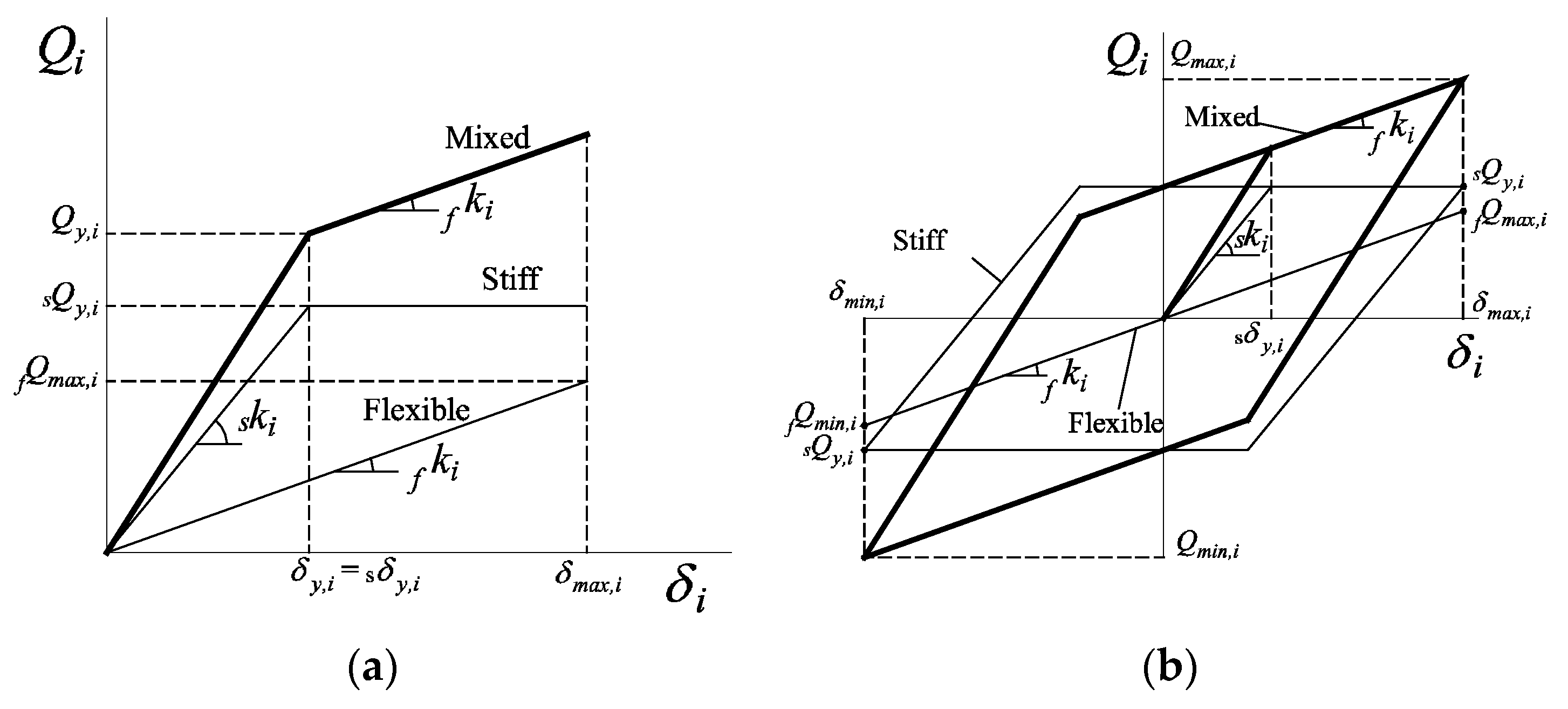
2.1. Idealization of a Structure with Metallic Dampers
2.2. Energy-Based Design Framework
2.3. Hysteretic Energy Accumulated under Cyclic and under Monotonic Loads
3. Proposal of New Optimum Yield-Shear Force Coefficient Distribution
4. Numerical Validation
4.1. Prototype Structures, Modelization and Ground Motions
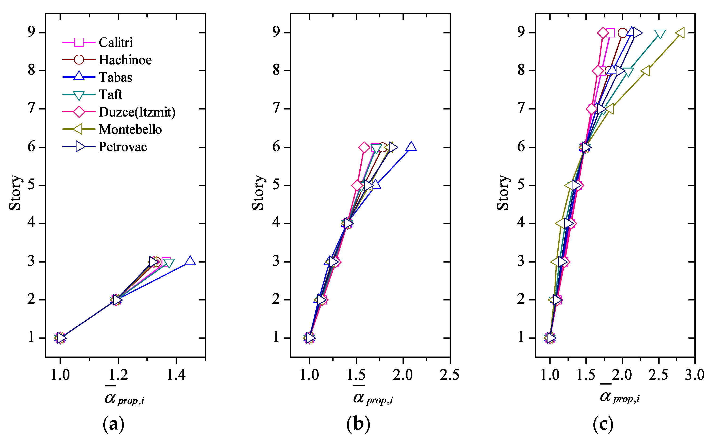
4.2. Optimum Distributions Obtained with the Proposed Expression for Different Ground Motions
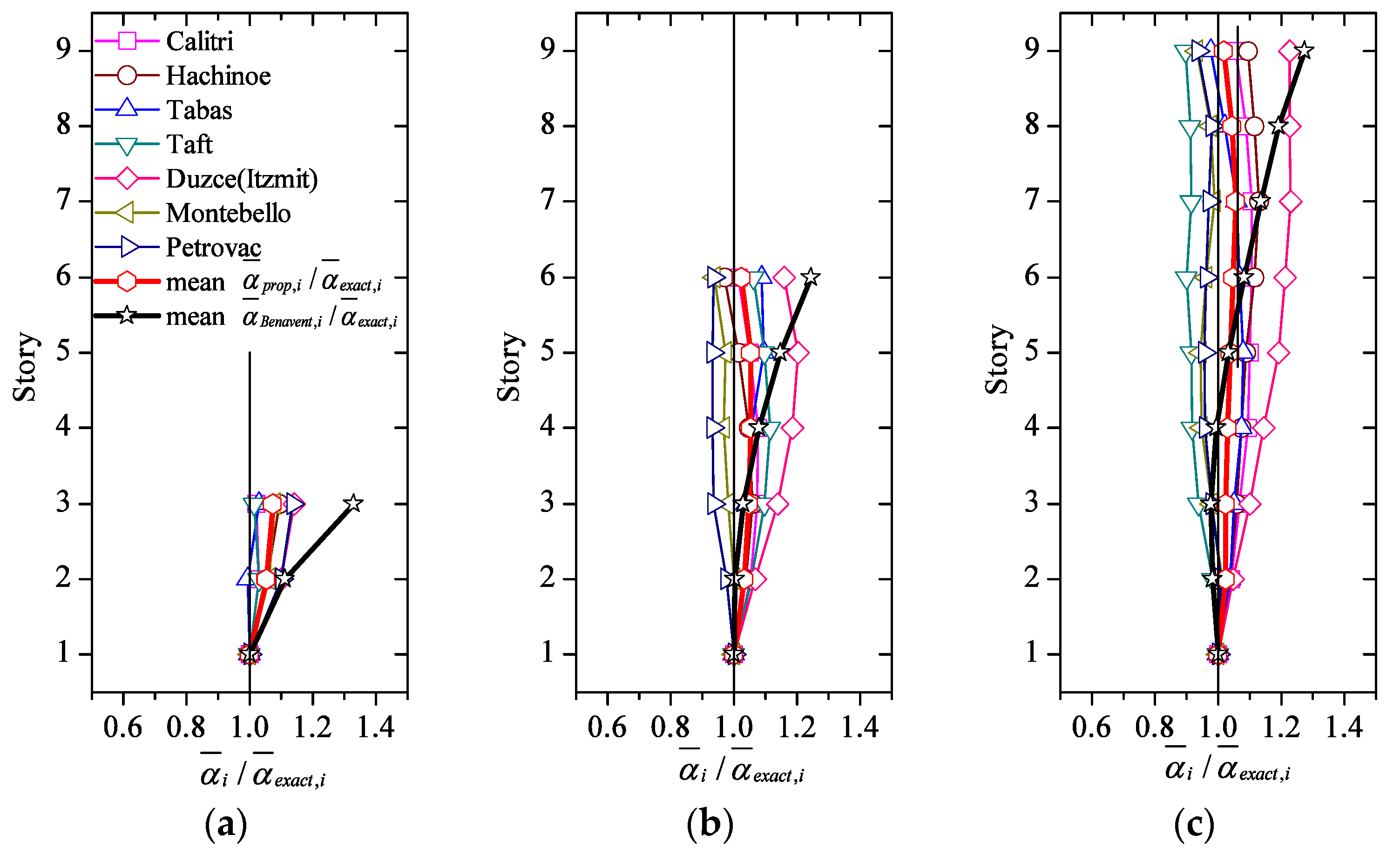
4.3. Comparison between Proposed and “Exact” Distributions
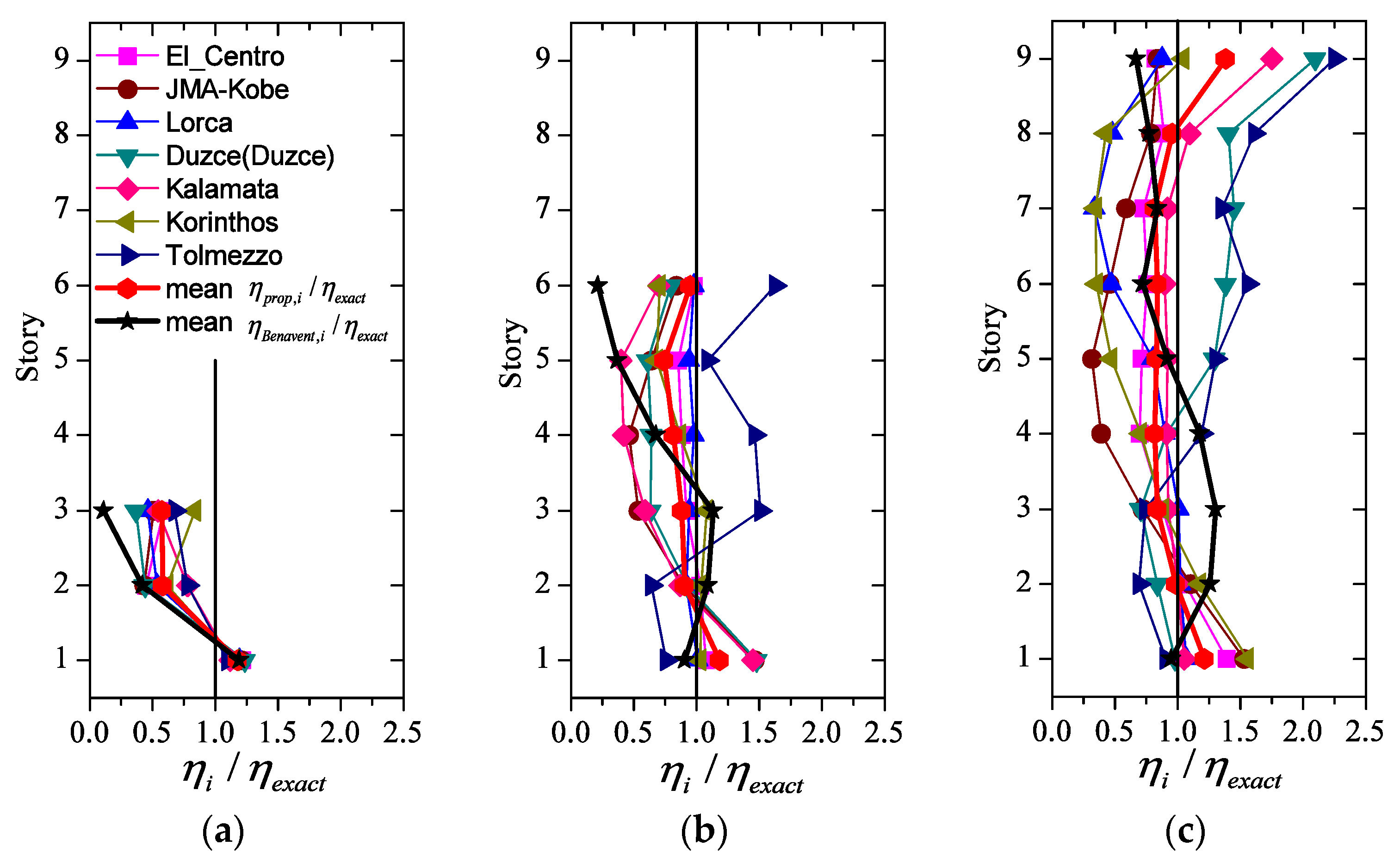
4.4. Damage Distribution among Stories
4.5. Maximum Interstory Drifts
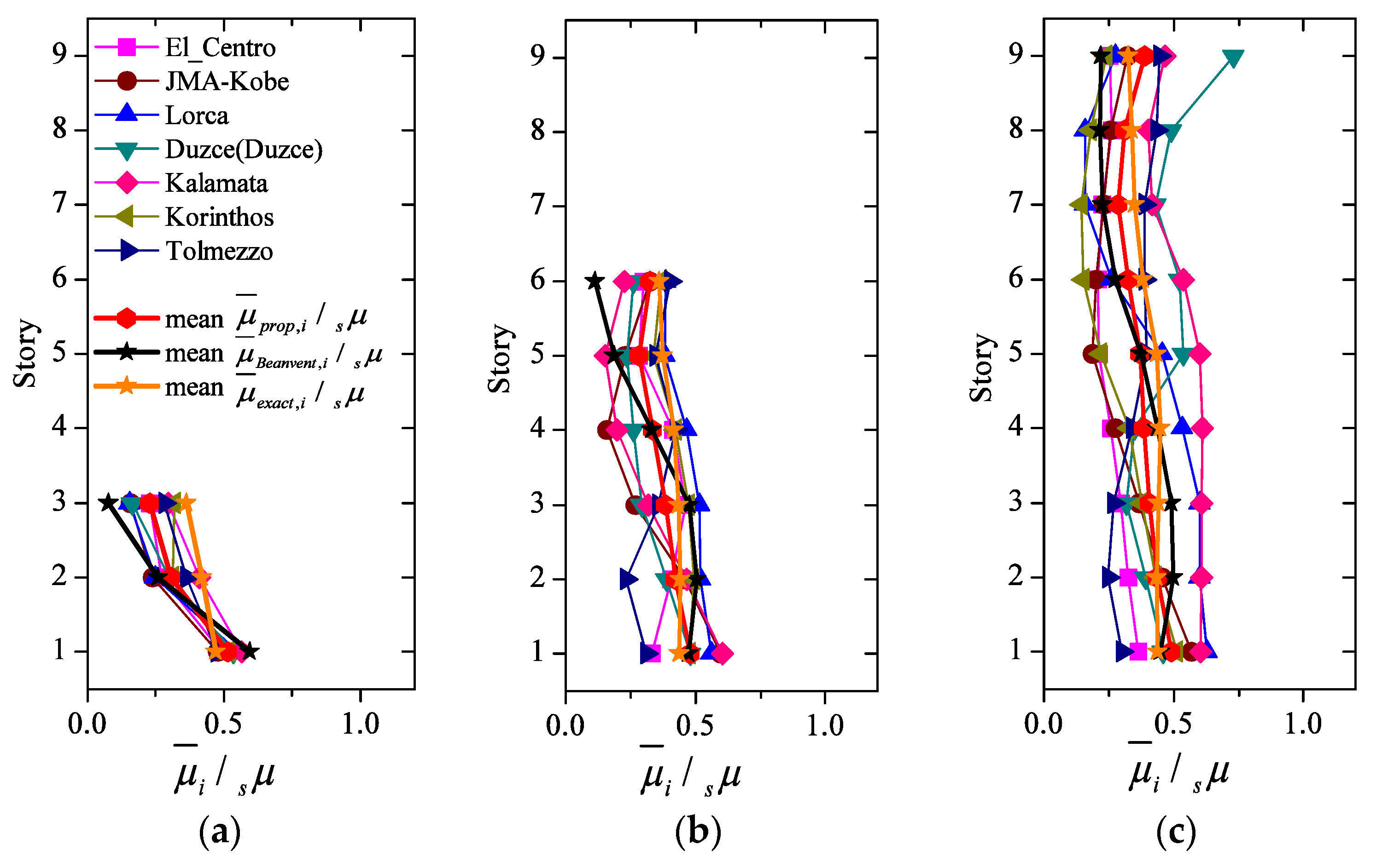
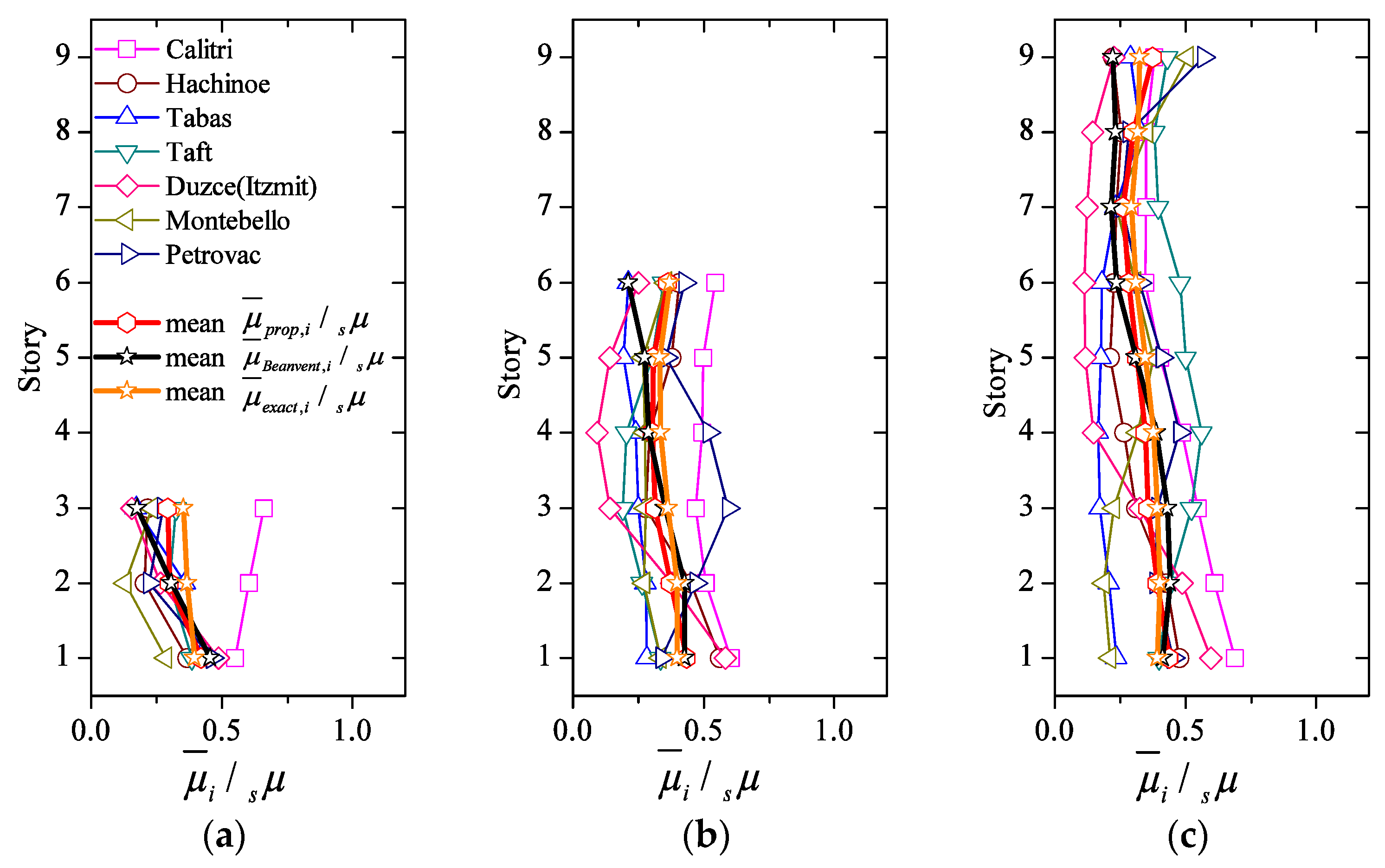
4.6. Ductility Distribution among Stories
5. Experimental Validation
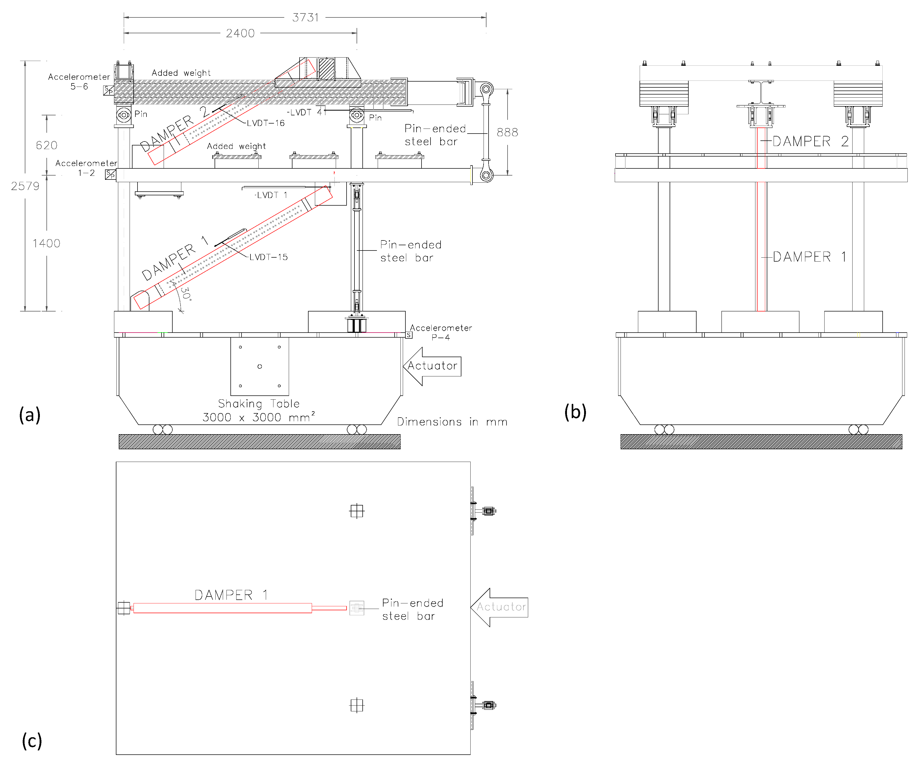
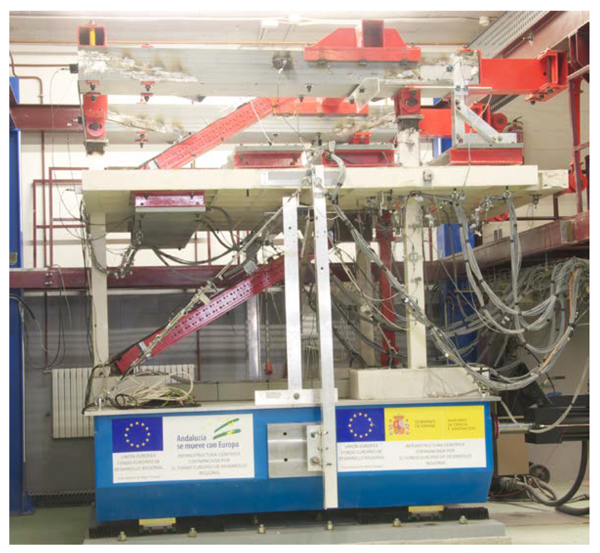
5.1. Test Model
5.2. Test Set-Up and Instrumentation
5.3. Seismic Simulations
5.4. Test Results
5.5. Discussion
6. Conclusions
- (1)
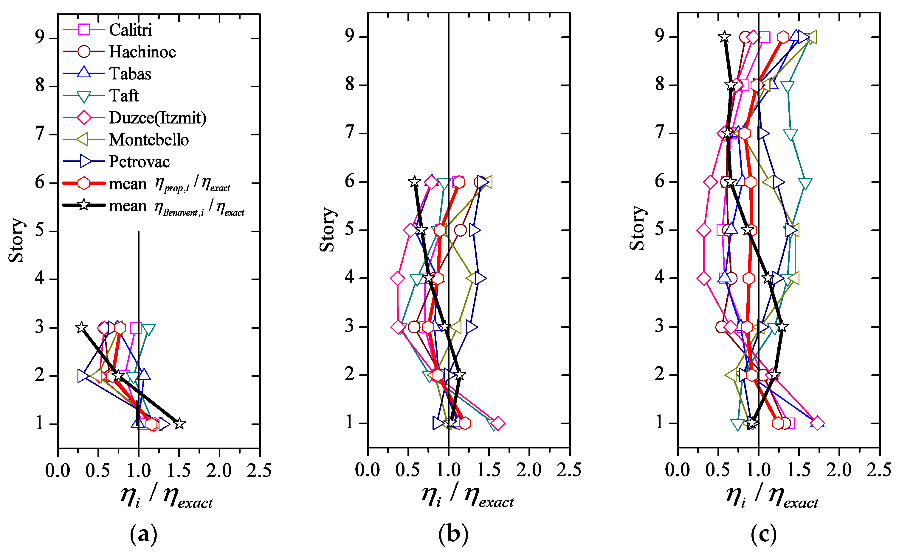
- is in good agreement with ; the ratio ranges between 0.9 to 1.2 and the coefficient of variation (COV) is less than 0.10;
- (2)
- improves significantly upon the one proposed by Benavent-Climent. , particularly for the upper 1/3 of the height of the structure.
- (3)
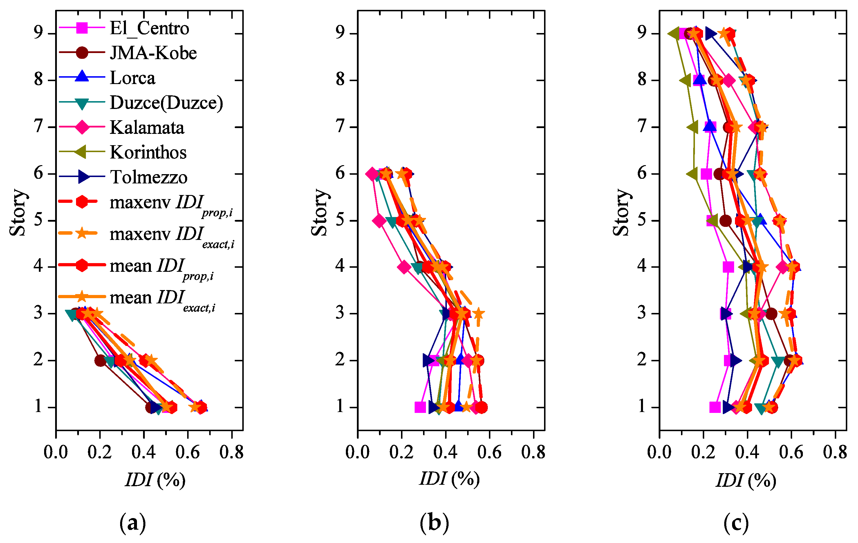
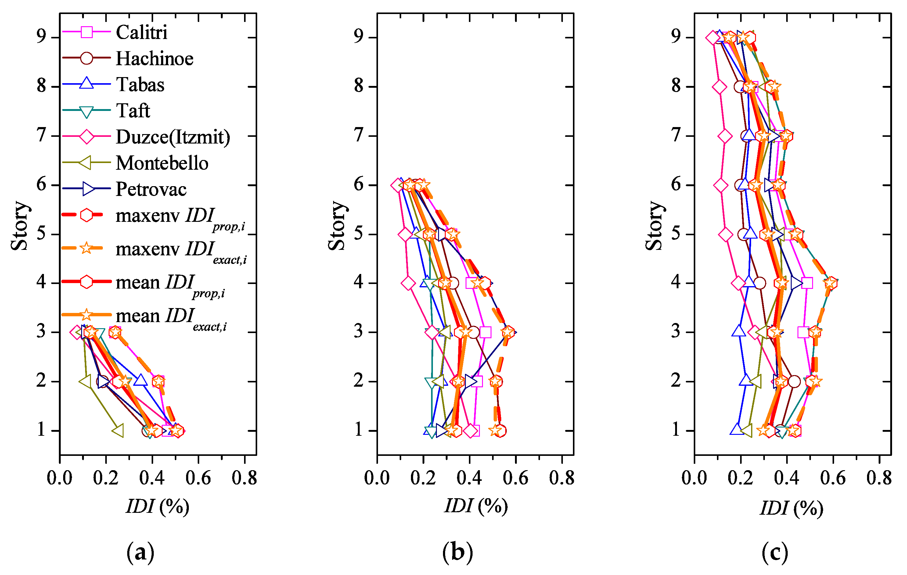
- The interstory-drifts of the structures designed with or with are very similar.
- (4)
- Deviations of the yield-shear force coefficient distribution with respect to , inevitably causes deviations of ηi from the aspired even distribution of damage (i.e., ηi = η equal in all stories). Nonetheless, if such deviations of the yield-shear force coefficient distribution are less than about 20%: (i) the variations of ηi among stories are small, thus damage concentration becomes a minor problem, and (ii) the inter-story drifts scarcely deviate from those obtained with
- (5)
- In structures having the optimum yield-shear force distribution, the ductility demand is approximately the same for all stories.
Author Contributions
Funding
Conflicts of Interest
Appendix A

| Earthquake | Record | Country | Year | TNH (s) | TG (s) | PGA (cm2/s) | PGV (cm2/s) | ID |
|---|---|---|---|---|---|---|---|---|
| El Centro | El Centro | EE.UU | 1940 | 0.60 | 0.46 | 341.31 | 37.23 | 8.95 |
| Hyogo-ken Nanbu | Kobe | Japan | 1995 | 0.84 | 0.34 | 820.32 | 90.24 | 7.11 |
| Lorca | Lorca | Spain | 2011 | 0.43 | 0.46 | 325.84 | 35.40 | 2.40 |
| Friuli | Tolmezzo | Italy | 1976 | 0.51 | 0.27 | 349.85 | 20.96 | 6.80 |
| Alkion | Korinthos | Greece | 1981 | 0.80 | 0.54 | 225.66 | 22.43 | 7.89 |
| Duzce | Duzce | Turkey | 1999 | 0.70 | 0.43 | 369.88 | 35.72 | 12.17 |
| Kalamata | Kalamata | Greece | 1986 | 0.50 | 0.56 | 327.50 | 25.97 | 3.01 |
| Earthquake | Record | Country | Year | TNH (s) | TG (s) | PGA (cm2/s) | PGV (cm2/s) | ID |
|---|---|---|---|---|---|---|---|---|
| Izmit | Duzce | Turkey | 1999 | 0.60 | 0.35 | 303.77 | 41.35 | 5.11 |
| Northridge | Montebello | EE.UU. | 1994 | 0.39 | 0.30 | 163.34 | 11.02 | 11.22 |
| Montenegro | Petrovac | Montenegro | 1979 | 0.64 | 0.46 | 445.30 | 38.37 | 16.54 |
| Tokachi-oki | Hachinoe | Japan | 1968 | 0.35 | 0.49 | 224.39 | 43.19 | 5.82 |
| Kern County | Taft | EE.UU. | 1952 | 0.70 | 0.35 | 152.90 | 17.15 | 12.97 |
| Campano Lucano | Calitri | Italy | 1980 | 1.00 | 1.20 | 155.00 | 26.16 | 16.51 |
| Tabas | Tabas | Iran | 1978 | 0.25 | 0.30 | 908.35 | 84.34 | 9.75 |
Appendix B

- (1)
- A tentative value is adopted for α0 taking into account that 0 < α0 < 1.
- (2)
- tAB is obtained from Equation (A8) and the result, together with α0, is used in Equation (A10) to obtain µiter.
- (3)
- If µiter = µtarget (with a fixed tolerance) the valid value for α0 is found, used in Equation (A9) to obtain Tmax. If not, the procedure is repeated from step 1 with a new value for α0.
References
- Veletsos, A.; Newmark, N.M. Effect of inelastic behavior on the response of simple systems to earthquake motions. In Proceedings of the 2nd World Conference on Earthquake Engineering; Earthquake Engineering Research Institute: Tokyo, Japan, 1960; pp. 895–912. [Google Scholar]
- CEN. European standard EN 1998-1:2004 Eurocode 8: Design of structures for earthquake resistance; European Committee for Standardization: Brussels, Belgium, 2005. [Google Scholar]
- Uang, C.-M.; Bertero, V.V. Evaluation of seismic energy in structures. Earthq. Eng. Struct. Dyn. 1990, 19, 77–90. [Google Scholar] [CrossRef]
- Kuntz, G.L.; Browning, J.A. Reduction of column yielding during earthquakes for reinforced concrete frames. ACI Struct. J. 2003, 100, 573–580. [Google Scholar]
- Fardis, M.N. From force-to displacement-based seismic desing of concrete structures and beyond. In Proceedings of the 16 European Conference on Earthquake Engineering; Springer: Thessaloniki, Greece, 2018; pp. 1–20. [Google Scholar]
- Housner, G.W. Limit Design of Structures to Resist Earthquakes. In Proceedings of the 1st WCEE; Earthquake Engineering Research Institute: Oakland, CA, USA, 1956; pp. 1–13. [Google Scholar]
- Akiyama, H. Earthquake resistant limit-state design for buildings (English Version); University of Tokyo Press: Tokyo, Japan, 1985. [Google Scholar]
- Building Research Institute. Earthquake-resistant structural calculation based on energy balance. In The Building Standard Law of Japan; The Building Center of Japan: Tokyo, Japan, 2009; pp. 414–423. [Google Scholar]
- De Domenico, D.; Ricciardi, G.; Takewaki, I. Design strategies of viscous dampers for seismic protection of building structures: A review. Soil Dyn. Earthq. Eng. 2019, 118, 144–165. [Google Scholar] [CrossRef]
- Deguchi, Y.; Kawashima, T.; Yamanari, M.; Ogawa, K. Sesimic design load distribution in steel frame. In Proceedings of the 14th World Conference on Earthquake Engineering, Beijing, China, 12–17 October 2008. [Google Scholar]
- Building Research Institute. Notification No. 1793 (1980): Stipulation of the value of Z, methods of calculating and Rt and Ai and standards for the designation by the Designated Administrative Organization of districts where the ground is extremely soft. In The Building Standard Law of Japan; The Building Center of Japan, Ed.; The Building Center of Japan: Tokyo, Japan, 2009; pp. 42–43. [Google Scholar]
- Benavent-Climent, A. An energy-based method for seismic retrofit of existing frames using hysteretic dampers. Soil Dyn. Earthq. Eng. 2011, 31, 1385–1396. [Google Scholar] [CrossRef]
- Kuwamura, H.; Galambos, T. Earthquake load for structural reliability. J. Struct. Eng. 1989, 115, 1446–1462. [Google Scholar] [CrossRef]
- Fajfar, P.; Vidic, T. Consistent inelastic design spectra: Hysteretic and input energy. Earthq. Eng. Struct. Dyn. 1994, 23, 523–537. [Google Scholar] [CrossRef]
- Lawson, R.; Krawinkler, H. Cumulative damage potential of seismic ground motion. In Proceedings of the 10th European Conference on Earthquake Engineering; Balkema: Vienna, Austria, 1995; pp. 1079–1086. [Google Scholar]
- Decanini, L.D.; Mollaioli, F. An energy-based methodology for the assessment of seismic demand. Soil Dyn. Earthq. Eng. 2001, 21, 113–137. [Google Scholar] [CrossRef]
- Benavent-Climent, A.; López-Almansa, F.; Bravo-González, D.A. Design energy input spectra for moderate-to-high seismicity regions based on Colombian earthquakes. Soil Dyn. Earthq. Eng. 2010, 30, 1129–1148. [Google Scholar] [CrossRef]
- López-Almansa, F.; Yazgan, A.U.; Benavent-Climent, A. Design energy input spectra for high seismicity regions based on Turkish registers. Bull. Earthq. Eng. 2013, 11, 885–912. [Google Scholar] [CrossRef]
- Chou, C.-C.; Uang, C.-M. A procedure for evaluating seismic energy demand of framed structures. Earthq. Eng. Struct. Dyn. 2003, 32, 229–244. [Google Scholar] [CrossRef]
- De Domenico, D.; Ricciardi, G. Dynamic response of non-classically damped structures via reduced-order complex modal analysis: Two novel truncation measures. J. Sound Vib. 2019, 452, 169–190. [Google Scholar] [CrossRef]
- Ministerio Fomento. Código Técnico de la Edificación. Documento Básico SE-AE; Centro Publicaciones. Secretaria General Técnica. M.Fomento: Madrid, Spain, 2008. [Google Scholar]
- Ministerio Fomento. Instrucción de Hormigón Estructural. EHE-08; Centro Publicaciones. Secretaria General Técnica. M.Fomento: Madrid, Spain, 2008. [Google Scholar]
- Cosenza, E.; Manfredi, G. Damage indices and damage measures. Prog. Struct. Eng. Mater. 2000, 2, 50–59. [Google Scholar] [CrossRef]
- SEAOC. Vision 2000: Performance Based Seismic Engineering of Buildings (VOL. 1), Prepared by Vision 2000 Committee; SEAOC: Sacramento, CA, USA, 1995. [Google Scholar]
- Benavent-Climent, A.; Donaire-Avila, J.; Oliver-Saiz, E. Shaking table tests of a reinforced concrete waffle-flat plate structure designed following modern codes: Seismic performance and damage evaluation. Earthq. Eng. Struct. Dyn. 2016, 45, 315–336. [Google Scholar] [CrossRef]
- Benavent-Climent, A.; Donaire-Avila, J.; Oliver-Sáiz, E. Seismic performance and damage evaluation of a waffle-flat plate structure with hysteretic dampers through shake-table tests. Earthq. Eng. Struct. Dyn. 2018, 47, 1250–1269. [Google Scholar] [CrossRef]
- Benavent-Climent, A.; Galé-Lamuela, D.; Donaire-Avila, J. Energy capacity and seismic performance of RC waffle-flat plate structures under two components of far-field ground motions: Shake table tests. Earthq. Eng. Struct. Dyn. 2019, 48, 949–969. [Google Scholar] [CrossRef]
- San, B.; Waisman, H.; Harari, I. Analytical and numerical shape optimization of a class of structures under mass constraints and self-weight. J. Eng. Mech. 2020, 146, 04019109. [Google Scholar] [CrossRef]
- Ehsani, A.; Dalir, H. Multi-objective optimization of composite angle grid plates for maximum buckling load and minimum weight using genetic algorithms and neural networks. Compos. Struct. 2019, 229, 111450. [Google Scholar] [CrossRef]
- Michael, R.; Torczon, V.; Trosset, M.W. Direct search methods: Then and now. J. Comput. Appl. Math. 2000, 124, 191–207. [Google Scholar]
- Kokil, A.S.; Shrikhande, M. Optimal placement of supplemental dampers in seismic design of structures. J. Seismol. Earthq. Eng. 2007, 9, 125–135. [Google Scholar]
- Bagheri, A.; Amini, F. Control of structures under uniform hazard earthquake excitation via wavelet analysis and pattern search method. Struct. Control. Heal. Monit. 2013, 20, 671–685. [Google Scholar] [CrossRef]
- Kourehli, S.S.; Amiri, G.G.; Ghafory-Ashtiany, M.; Bagheri, A. Structural damage detection based on incomplete modal data using pattern search algorithm. J. Vib. Control 2013, 19, 821–833. [Google Scholar] [CrossRef]
- Benavent-Climent, A.; Morillas, L.; Vico, J. A study on using wide-flange section web under out-of-plane flexure for passive energy dissipation. Earthq. Eng. Struct. Dyn. 2011, 40, 473–490. [Google Scholar] [CrossRef]
- Forum-8. Engineer’s Studio V.1.07.02 (Computer Program.); FORUM-8: London, UK, 2012. [Google Scholar]


| Prototype | 3-Story | 6-Story | 9-Story | ||||||
|---|---|---|---|---|---|---|---|---|---|
| Story | fki (kN/cm) | mi (kNs2/cm) | hi (m) | fki(kN/cm) | mi (kNs2/cm) | hi (m) | fki(kN/cm) | mi (kNs2/cm) | hi (m) |
| 9 | - | - | - | - | - | - | 1523 | 5.24 | 3.10 |
| 8 | - | - | - | - | - | - | 1572 | 5.68 | 3.10 |
| 7 | - | - | - | - | - | - | 1618 | 5.68 | 3.10 |
| 6 | - | - | - | 1071 | 3.51 | 3.10 | 2149 | 5.68 | 3.10 |
| 5 | - | - | - | 1120 | 3.89 | 3.10 | 2191 | 5.68 | 3.10 |
| 4 | - | - | - | 1126 | 3.89 | 3.10 | 2206 | 5.68 | 3.10 |
| 3 | 571 | 2.22 | 3.10 | 1141 | 3.89 | 3.10 | 2707 | 5.68 | 3.10 |
| 2 | 569 | 2.56 | 3.10 | 1518 | 3.89 | 3.10 | 2803 | 5.68 | 3.10 |
| 1 | 510 | 2.56 | 3.50 | 1636 | 3.89 | 3.50 | 3259 | 5.68 | 3.50 |
| fT1 (s) | 0.94 | 1.38 | 1.81 | ||||||
| Records | SF | K | T1 (s) | VD (cm/s) | sα1 | η | sμ |
|---|---|---|---|---|---|---|---|
| Near-Field | - | - | - | - | - | - | - |
| El Centro | 0.90 | 6.6 | 0.34 | 65 | 0.18 | 15.7 | 5.7 |
| Kobe | 0.35 | 8.1 | 0.31 | 66 | 0.18 | 19.0 | 7.1 |
| Lorca | 1.00 | 8.5 | 0.31 | 53 | 0.22 | 7.5 | 5.9 |
| Tolmezzo | 1.25 | 8.3 | 0.31 | 60 | 0.18 | 16.1 | 7.4 |
| Korinthos | 1.00 | 4.1 | 0.42 | 60 | 0.16 | 10.3 | 3.8 |
| Duzce (Duzce) | 0.75 | 11.0 | 0.27 | 79 | 0.18 | 42.3 | 10.4 |
| Kalamata | 1.00 | 4.7 | 0.39 | 49 | 0.16 | 7.0 | 4.6 |
| Far-Field | - | - | - | - | - | - | |
| Duzce (Izmit) | 1.00 | 9.6 | 0.29 | 55 | 0.18 | 14.4 | 8.6 |
| Montebello | 1.75 | 12.2 | 0.26 | 65 | 0.17 | 30.8 | 12.0 |
| Petrovac | 0.50 | 7.7 | 0.32 | 80 | 0.16 | 37.3 | 7.8 |
| Hachinoe | 0.95 | 7.7 | 0.32 | 53 | 0.18 | 10.7 | 6.9 |
| Taft | 1.00 | 1.8 | 0.56 | 52 | 0.07 | 16.3 | 3.8 |
| Calitri | 1.00 | 1.6 | 0.58 | 60 | 0.05 | 38.1 | 4.8 |
| Tabas | 0.40 | 6.0 | 0.36 | 55 | 0.18 | 9.0 | 5.0 |
| Records | SF | K | T1 (s) | VD (cm/s) | sα1 | η | sμ |
|---|---|---|---|---|---|---|---|
| Near-Field | - | - | - | - | - | - | - |
| El Centro | 0.70 | 3.7 | 0.64 | 65 | 0.13 | 6.6 | 2.9 |
| Kobe | 0.30 | 5.9 | 0.52 | 69 | 0.14 | 11.3 | 4.9 |
| Lorca | 1.00 | 6.0 | 0.52 | 46 | 0.06 | 18.1 | 12.9 |
| Tolmezzo | 1.58 | 4.6 | 0.58 | 66 | 0.17 | 5.0 | 2.9 |
| Korinthos | 1.20 | 4.5 | 0.59 | 69 | 0.15 | 6.9 | 3.1 |
| Duzce (Duzce) | 0.75 | 7.9 | 0.46 | 83 | 0.14 | 23.3 | 6.9 |
| Kalamata | 1.30 | 17.7 | 0.32 | 65 | 0.17 | 18.9 | 13.3 |
| Far-Field | - | - | - | - | - | - | - |
| Duzce (Izmit) | 1.00 | 12.2 | 0.38 | 65 | 0.17 | 12.9 | 8.8 |
| Montebello | 2.30 | 7.5 | 0.47 | 72 | 0.18 | 9.4 | 5.0 |
| Petrovac | 0.62 | 2.0 | 0.80 | 64 | 0.07 | 13.5 | 3.3 |
| Hachinoe | 1.10 | 3.4 | 0.66 | 53 | 0.14 | 3.2 | 2.4 |
| Taft | 1.70 | 8.2 | 0.45 | 81 | 0.14 | 22.6 | 7.3 |
| Calitri | 1.00 | 2.9 | 0.70 | 76 | 0.06 | 32.3 | 5.3 |
| Tabas | 0.40 | 6.8 | 0.49 | 63 | 0.12 | 12.8 | 7.1 |
| Records | SF | K | T1 (s) | VD (cm/s) | sα1 | η | sμ |
|---|---|---|---|---|---|---|---|
| Near-Field | - | - | - | - | - | - | - |
| El Centro | 0.90 | 7.8 | 0.61 | 85 | 0.15 | 10.9 | 5.2 |
| Kobe | 0.36 | 10.7 | 0.53 | 86 | 0.15 | 15.7 | 7.6 |
| Lorca | 1.60 | 6.0 | 0.68 | 62 | 0.10 | 9.3 | 7.3 |
| Tolmezzo | 1.80 | 5.0 | 0.74 | 76 | 0.15 | 5.3 | 3.2 |
| Korinthos | 1.50 | 16.7 | 0.43 | 90 | 0.15 | 28.1 | 12.5 |
| Duzce (Duzce) | 0.90 | 2.9 | 0.92 | 79 | 0.10 | 7.8 | 2.8 |
| Kalamata | 1.20 | 6.0 | 0.68 | 53 | 0.05 | 25.4 | 15.7 |
| Far-Field | - | - | - | - | - | - | - |
| Duzce (Izmit) | 1.10 | 17.6 | 0.42 | 75 | 0.15 | 18.9 | 13.2 |
| Montebello | 3.30 | 5.0 | 0.74 | 74 | 0.12 | 8.2 | 4.4 |
| Petrovac | 0.80 | 4.2 | 0.79 | 87 | 0.10 | 14.3 | 4.3 |
| Hachinoe | 1.20 | 7.1 | 0.64 | 67 | 0.12 | 8.9 | 6.3 |
| Taft | 1.85 | 2.1 | 1.03 | 69 | 0.06 | 9.6 | 3.2 |
| Calitri | 1.00 | 4.1 | 0.80 | 92 | 0.08 | 20.8 | 4.7 |
| Tabas | 0.35 | 8.8 | 0.58 | 75 | 0.15 | 9.5 | 6.3 |
| Type of Records | Near-Field | Far-Field | ||||
|---|---|---|---|---|---|---|
| Prototypes | N | N | ||||
| 3 | 6 | 9 | 3 | 6 | 9 | |
| COV of “mean ” | 0.10 | 0.08 | 0.12 | 0.05 | 0.07 | 0.11 |
| COV of “mean ” | 0.35 | 0.18 | 0.16 | 0.18 | 0.14 | 0.16 |
| COV of “mean ” | 0.69 | 0.43 | 0.32 | 0.36 | 0.24 | 0.28 |
© 2020 by the authors. Licensee MDPI, Basel, Switzerland. This article is an open access article distributed under the terms and conditions of the Creative Commons Attribution (CC BY) license (http://creativecommons.org/licenses/by/4.0/).
Share and Cite
Donaire-Ávila, J.; Benavent-Climent, A. Optimum Strength Distribution for Structures with Metallic Dampers Subjected to Seismic Loading. Metals 2020, 10, 127. https://doi.org/10.3390/met10010127
Donaire-Ávila J, Benavent-Climent A. Optimum Strength Distribution for Structures with Metallic Dampers Subjected to Seismic Loading. Metals. 2020; 10(1):127. https://doi.org/10.3390/met10010127
Chicago/Turabian StyleDonaire-Ávila, Jesús, and Amadeo Benavent-Climent. 2020. "Optimum Strength Distribution for Structures with Metallic Dampers Subjected to Seismic Loading" Metals 10, no. 1: 127. https://doi.org/10.3390/met10010127
APA StyleDonaire-Ávila, J., & Benavent-Climent, A. (2020). Optimum Strength Distribution for Structures with Metallic Dampers Subjected to Seismic Loading. Metals, 10(1), 127. https://doi.org/10.3390/met10010127