Approaches to Modeling of Recrystallization


Abstract
: Control of the material microstructure in terms of the grain size is a key component in tailoring material properties of metals and alloys and in creating functionally graded materials. To exert this control, reliable and efficient modeling and simulation of the recrystallization process whereby the grain size evolves is vital. The present contribution is a review paper, summarizing the current status of various approaches to modeling grain refinement due to recrystallization. The underlying mechanisms of recrystallization are briefly recollected and different simulation methods are discussed. Analytical and empirical models, continuum mechanical models and discrete methods as well as phase field, vertex and level set models of recrystallization will be considered. Such numerical methods have been reviewed previously, but with the present focus on recrystallization modeling and with a rapidly increasing amount of related publications, an updated review is called for. Advantages and disadvantages of the different methods are discussed in terms of applicability, underlying assumptions, physical relevance, implementation issues and computational efficiency.1. Introduction
The macroscopic behavior of metallic materials is to a large extent controlled by the size and shape of the grains that constitute the material microstructure. The microlevel grain structure will influence macroscopic material properties such as mechanical strength, electrical conductivity, wear and corrosion resistance, ductility, hardness and fatigue resistance. Being able to predict and control the morphology of this microstructure during different metal working processes thus allows the development of tailored material properties, optimized products and more efficient production processes. Understanding and manipulating the material microstructure are key components in the production of functionally graded materials, having engineered properties in different regions.
Fine-grained materials, with grain sizes down to the nanoscale, are becoming increasingly important in many applications, e.g., in the miniaturization of products such as micro-electro-mechanical components (MEMS), in biomedical devices and also in the production of thin metallic films and foils. As one or more physical dimensions of the product are reduced, the microstructure has to be tailored correspondingly in order to maintain required material properties and reliable operation of the product. Recrystallization and grain size control is also of primary interest in the development of high strength steels. From these observations it is clear that grain size and recrystallization are fundamental concepts in materials science and in materials design.
Recognizing that grain refinement through recrystallization can be achieved by exposing the material to severe plastic deformation, several processes such as equal channel angular pressing (ECAP), asymmetric rolling (ASR), accumulated roll bonding (ARB) and high pressure torsion (HPT) have been devised. In order to optimize such processes and to gain further insight into the mechanics of recrystallization, physically motivated and computationally efficient simulation models are vital. Simulations can be used to predict the microstructure evolution, e.g., in terms of grain size and relative grain misorientation, during plastic deformation and also to indicate suitable settings of process parameters such as deformation magnitude, deformation rate and processing temperature. In addition, crystallographic texture, kinetics of grain boundary migration and the size and distribution of second-phase precipitates can be studied through simulation.
The existence and importance of recrystallization as a metallurgical process has been recognized for many years and simulation models of the process continue to evolve and new techniques continuously emerge. This is of course due to the increased knowledge of the physics behind the process but also due to the increasing availability of efficient computer resources. Review papers considering various approaches to recrystallization modeling have been published previously. In [1], the focus lies on Monte Carlo Potts models and on a vertex model formulated by the author. Cellular automata and vertex methods are mentioned in [2] but the focus lies on Monte Carlo Potts models. Monte Carlo Potts models and cellular automata are also the topic in [3]. Recrystallization modeling using Monte Carlo Potts methods, with particular application to aluminum alloys, is considered in [4] where also vertex and phase field models are discussed.
The present paper aims at providing an updated review of various approaches to modeling and simulation of recrystallization. Continuum mechanical models, cellular automata and Monte Carlo Potts methods as well as more recent methods such as phase field formulations, vertex and level set models are considered. Advantages and disadvantages of the different approaches are discussed. Although the present paper focuses on numerical models, some attention is also given to analytical and empirical models and classical descriptions of recrystallization. Combined formulations such as crystal plasticity/cellular automata models and multi-level simulations using, e.g., cellular automata with finite elements or crystal plasticity models connected to phase field formulations are not considered here since this is beyond the scope of this review paper. But in passing it is recognized that such multi-level simulations provide promising tools to connect macroscopic structural behavior with a detailed description of the microstructural evolution in a material during deformation. Nor is anything discussed on molecular dynamics simulations which have been used to some extent in the study of the details of separate processes during recrystallization. Several of the herein considered approaches are mainly used to model the material behavior on the grain size level. These models can in many cases be employed in simulations using representative volume elements from which the macroscopic material behavior can be estimated through averaging of quantities defining the microstructure. Such homogenization procedures are not covered here.
This review paper begins in Section 2 with a brief discussion on the recrystallization process itself. This is by no means an in-depth description of the complex recrystallization phenomena but highlights the essential features to be captured in modeling of the process. In Section 3, classical and empirical approaches to modeling of recrystallization are mentioned and fundamental results related to the nucleation of recrystallization grains, to grain growth and to grain boundary kinetics are given. Section 4 discusses continuum mechanical models. Monte Carlo Potts models are the topic of Section 5 and cellular automata of Section 6. Section 7 outlines some fundamental features of phase field formulations and Section 8 gives some notes on vertex, or front-tracking, models. Level set models are the topic of Section 9. Some concluding remarks are given in Section 10. Each of the topics mentioned represent active fields of research and in-depth discussions on each field are beyond the scope of this review article where central concepts and especially applications to recrystallization are in focus. References for further reading are given throughout the text.
2. Mechanics of Recrystallization
As a metallic materials is deformed through plastic slip, energy will be accumulated in the material. This energy is to a large extent expended as heat while the remainder is stored in the material microstructure through the generation and redistribution of imperfections, mainly dislocations. With progressing plastic deformation, the material becomes increasingly thermodynamically unstable. A number of different processes are now active to reduce the stored energy. One of these processes is recrystallization, whereby new grains of relatively low stored energy are nucleated in the microstructure. These grain nuclei can under proper conditions grow to consume the high-energy microstructure in their surroundings, created by the macroscopic plastic deformation. Reducing the internally stored energy, the material is by recrystallization returned to a thermodynamically more favorable state.
Recrystallization is generally accepted to be defined as the formation of a new grain structure in a plastically deformed material. This recrystallization occurs through the formation and migration of high-angle boundaries, i.e., boundaries with a crystallographic misorientation greater than 10–15°. Boundary migration is driven by stored energy reduction and minimization of surface energy.
Recrystallization can take place as a relatively slow and temperature-driven process, subsequent to deformation, known as static recrystallization (SRX). Alternatively, during plastic deformation of the material, dynamic recrystallization (DRX) can take place [5,6]. Experimental investigations have shown that dynamic recrystallization can in fact be subdivided into two main, physically different, processes [7–9]. In materials of low stacking-fault energy, such as copper, dynamic recovery processes such as cross slip and climb are limited and the microstructural evolution is dominated by discontinuous dynamic recrystallization (DDRX) during which new grains are nucleated at high-energy sites in the microstructure. Nucleation occurs mainly along grain boundaries but also near second-phase particles and inclusions in the grain interiors, giving rise to particle-stimulated nucleation (PSN). In materials of high stacking-fault energy, such as aluminum, dynamic recovery is more influential and recrystallization occurs mainly by continuous dynamic recrystallization (CDRX). In this case, subgrains with low-angle boundaries are formed from dislocation networks. With progressing plastic deformation, misorientation is increased until enough energy is achieved and the initially mobile subgrain walls have become immobilized, allowing new grains to be separated. It is worth noting that DDRX and CDRX in some cases work together and that CDRX can act as a precursor to DDRX.
Once new grains have emerged, through either DDRX or CDRX, they may grow by grain boundary migration. A driving pressure acts on the grain boundaries due to the jumps in stored energy across the boundaries, allowing the new grains to expand. As grains grow, the grain boundary area and the related grain boundary energy will increase. This acts to lower the grain boundary migration rate and to reduce the grain size. The grain boundary migration kinetics are further complicated in the presence of particles which can give rise to drag forces on the boundaries and partially pin them down. This particle pinning will restrict the progression of recrystallization while, in contrast, particles (of larger size) also may be favorable to the recrystallization process through particle stimulated nucleation, as mentioned.
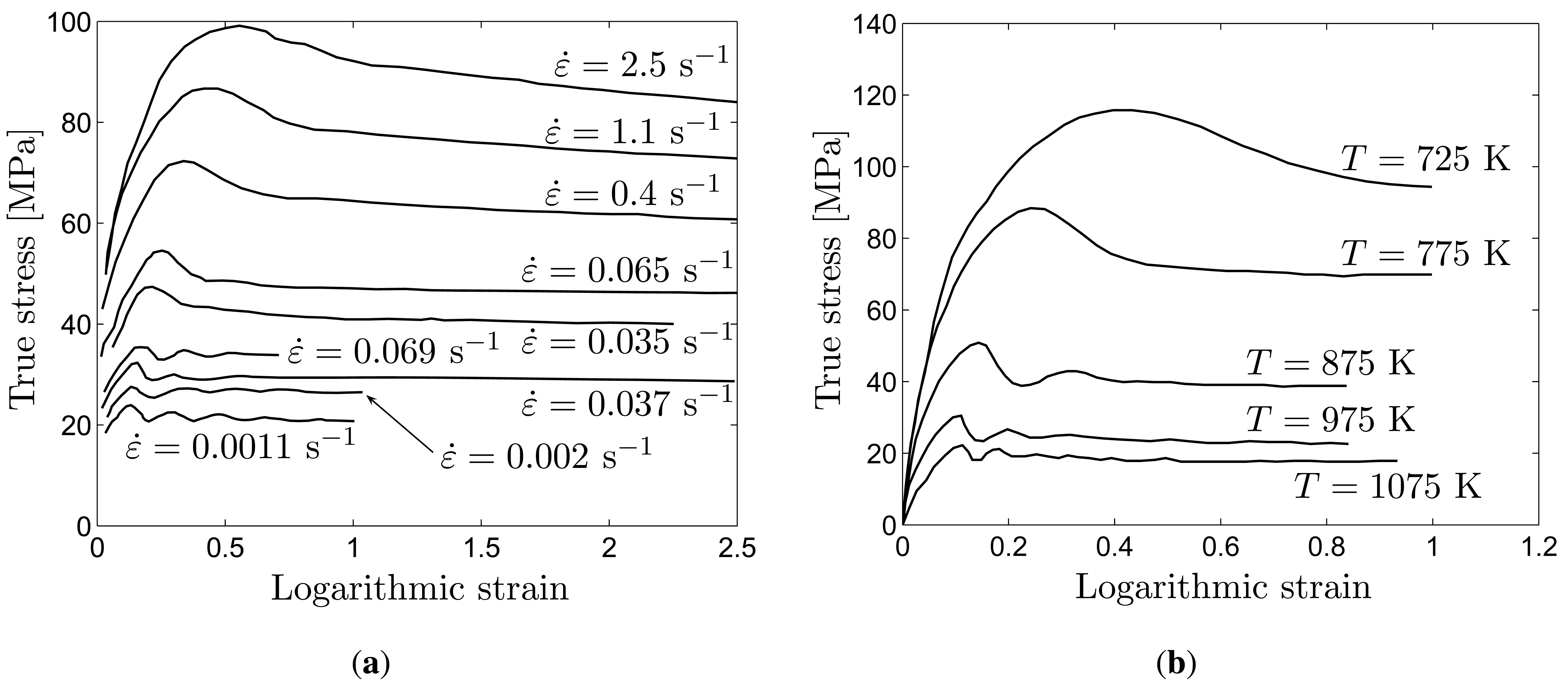
Some characteristics of the material behavior during recrystallization are worth noting since these should be anticipated in the results obtained from modeling and simulation of the recrystallization process. A first such characteristic is noted as new grains are nucleated at sites of high dislocation density during DDRX. This primarily occurs along grain boundaries whereby it is common to observe “necklace” patterns of recrystallized grains along these boundaries. Second, if a two-dimensional microstructure with homogeneously distributed stored energy is studied, and particle pinning effects are absent, grain growth will be purely curvature-driven. The evolution of the grain structure will be controlled solely by the minimization of interfacial energy. In this arrangement, the equilibrium state will consist of grains separated by boundaries connected at triple junctions with a 120° division between the boundaries. Finally, as new grains of lower dislocation density consume the microstructure deformed through plastic slip, the macroscopic flow stress behavior of the material will be altered. Caused by dynamic recrystallization, flow stress serrations will appear. At lower temperatures or increased strain-rates, cycles of recrystallization overlap and evens the flow stress oscillations. In this case single-peak flow, followed by dynamic softening is observed. At higher temperatures, or lower strain rates, each cycle of recrystallization is allowed to more or less finish before the next one sets in. This results in flow stress oscillations. In both cases the flow stress tends to saturate at some level, corresponding to a relatively stable saturation grain size. This is illustrated in Figure 1(a), showing experimental results taken from [10] on the flow stress behavior of a 0.25% carbon steel under varying strain-rates with the temperature held constant. Correspondingly, Figure 1(b) shows experimental results from [11] on OFHC copper where the strain-rate is held constant while changing the process temperature. In both cases the transition from single-peak flow stress behavior into multiple-peak serrated flow, can be observed. The dependence on process temperature and strain rate will obviously alter the recrystallization behavior as these parameters are changed. Estimation of optimum process parameters is hence an important motivation for modeling of recrystallization.
The process of recrystallization is discussed in depth in the review paper [5] and is thoroughly treated in [6]. Recrystallization modeling by different methods is also part of [12] and grain boundary migration and related topics are extensively discussed in [13].
3. Classical Results and Empirical Models
The kinetics of recrystallization is classically addressed using the Kolmogorov–Johnson–Mehl–Avrami (KJMA) relation [14–18]. By this approach, a variable X is introduced to describe the progress of recrystallization, i.e., the fraction of recrystallized material, with X = 0 at the onset of recrystallization and X = 1 for the fully recrystallized material. Having established the growth velocity and the rate of nucleation, the extent of recrystallization can be estimated. The KJMA model considers impingement of growing grains after which further growth of the grains is inhibited. To this end, an expanded volume is defined into which recrystallized grains can nucleate and grow. The expanded volume is allowed to contain previously recrystallized material. A differential relation is then established between the increment in recrystallized volume which would have been created in the absence of impingement and the true volume increment. Integration of this differential relation results in
As discussed in Section 2, temperature and strain rate are key parameters in recrystallization. Considering these parameters together, empirical models of recrystallization are often based on the Zener-Hollomon parameter, defined as
As mentioned previously, nucleation of new grains occurs at sites in the microstructure where enough stored energy is present. The complexity of the nucleation process often requires some simplifications to be made during modeling of the event. It is therefore common to see for example grain boundary serration, relative grain boundary motion (shearing and sliding) and twinning mechanisms be disregarded although being vital parts in the nucleation process [24–26]. Experimental studies have also indicated that the character of the nucleation process changes with temperature and rate of deformation which complicates the picture [27]. In addition, nucleation may also occur at a number of different sites in the microstructure, e.g., at grain boundaries, at triple junctions and near particle inclusions. Frequently only grain boundary nucleation is considered in recrystallization models. Particle stimulated nucleation is, however, considered in cellular automata simulations of recrystallization in [1,28].
Models that explicitly treat the nucleation event often consider a critical dislocation density ρc, needed for nucleation to take place [29–33]. In [29], this critical dislocation density is related to the macroscopic effective plastic strain according to
Considering a continuous nucleation process, rather than the site-saturated nucleation of the KJMA formulation, the rate of nucleation is conveniently related to the macroscopic effective plastic strain by a relation on the form
Once nucleated, the recrystallized grains can grow due to a driving pressure p acting on the grain boundary. The local velocity υ of a grain boundary can be written as
The pressure component due to particle drag appears on general form as
Purely curvature-driven grain boundary migration is considered for example in [46]. Impurity effects on grain boundary migration is discussed in the review paper [47] and also in [6,13]. Modeling of the influence on grain boundary migration kinetics from particle drag forces is discussed in the review paper [48] and in conjunction with Monte Carlo Potts modeling in [49], with cellular automata in [50] and using phase field formalism in [51–54].
The grain boundary mobility that enters Equation (6) is usually given a temperature dependence according to an Arrhenius relation on the form
The grain microstructure will influence the material behavior on several levels. Microscopically, the evolution of the dislocation density will be influenced by the grain size as grain boundaries pose obstacles to dislocation motion and serve as sites for dislocation accumulation and storage. Macroscopically, this will manifest itself in an influence on the flow stress behavior of the material, for example due to a Hall-Petch component. In addition, the macroscopic strain-rate dependence of the material will be influenced by the grain structure as shown for aluminum in [57].
4. Continuum Mechanical Models
In continuum mechanical models of inelastic material behavior, it is common to describe the deformation history by use of internal variables. These are often variables related to the accumulated plastic deformation and the macroscopic deformation hardening of the material. Different aspects of internal variable formulations are discussed in the review papers [58,59]. Considering such continuum mechanical formulations where recrystallization is also included, the internal variables can in addition represent other homogenized quantities such as the dislocation density and the grain size. Macroscopic properties such as flow stress behavior and strain-rate dependence will by this approach be linked to averaged properties of the evolving microstructure. The macroscopic flow stress σy will include a dependence on the average grain size d, often described by the Hall-Petch proportionality
In addition, during plastic deformation of the material, the increasing dislocation density ρd will be perceived macroscopically as a deformation hardening. This can be described by
The evolution of the dislocation density will also be influenced by the recrystallization process as the new grains are of considerably lower stored energy than the parent material. Also, when the average grain size decreases, the amount of grain boundary area will increase which results in restricted mobility of the dislocations and dislocation accumulation. The intricate relations between the different physical processes, and across length scales, result in a system of coupled equations that yield the evolution of the internal variables.
In several phenomenological continuum mechanical models of dynamic recrystallization, the critical condition for initiation of recrystallization is taken as a macroscopic critical plastic strain , corresponding to the critical dislocation density in Equation (4) on the microlevel. By this approach, recrystallization is not activated until . This approach is used in a finite strain, visco-plastic, constitutive model of recrystallization in [60]. Such a macroscopic recrystallization criterion is also discussed in relation to analytical models and experimental results in [61–63]. In [64], where SRX is modeled, the dislocation density is represented in terms of an internal variable related to the isotropic hardening of the material. A temperature-dependent critical threshold value of this variable is defined and as the isotropic hardening variable reaches the critical value, recrystallization is initiated. A similar model is established by the same group in [65], where both static and dynamic recrystallization is considered.
As the recrystallization criterion is met, the initial average grain size d0 will be gradually reduced until a saturation grain size df is reached. Frequently the evolution of the average grain size is described by an expression on the form
Another approach to describing the recrystallization process is related to the formulation in [71,72]. An evolution equation for the subgrain size δ is established according to
Continuum mechanical models where recrystallization is taken into account have the definite advantage of being able to conveniently simulate macroscopic structural behavior influenced by an evolving material microstructure. A further advantage of the continuum mechanical formulations is that they often are readily implemented as material models in existing finite element models. It is however less straight-forward to include microstructure parameters such as grain orientation and re-orientation during the macroscopic deformation process, i.e., the evolution of crystallographic texture. Such information can be obtained from crystal plasticity formulations where, however, the changes in microstructure in terms of nucleation, growth and consumption of grains is more of an issue. It is also worth noting that in continuum mechanical models, the characteristic parameters of the grain microstructure—such as grain size and dislocation density—are only available as homogenized quantities.
5. Monte Carlo Potts models
The Potts model [76] is an elaboration of the Ising model that in turn is based on the two states of a magnetic spin system to describe the evolution of a magnetic domain. In the Ising model, the analysis domain—in two or three dimensions—is discretized onto a grid of lattice sites, each characterized by its magnetic spin state, either up or down. Performing the simulation, the Ising model strives to minimize the presence of boundaries between regions of the two spin states. The Potts model is a generalization of the Ising model in the sense that an arbitrary number of Q spin states is considered. The Ising model is obviously obtained from the Potts model by the choice of Q = 2. In [77–79] it was recognized that the Potts model had all the characteristics of a polycrystalline grain structure and a Monte Carlo sampling of different states was introduced in conjunction with the Potts formulation. Monte Carlo Potts models are reviewed in [2,4] and the algorithm is also discussed in [12]. In [48], the Monte Carlo Potts model is used in a study of Zener pinning and is also compared to results from phase field and front tracking methods. Monte Carlo Potts modeling of particle pinning is also discussed in [49].
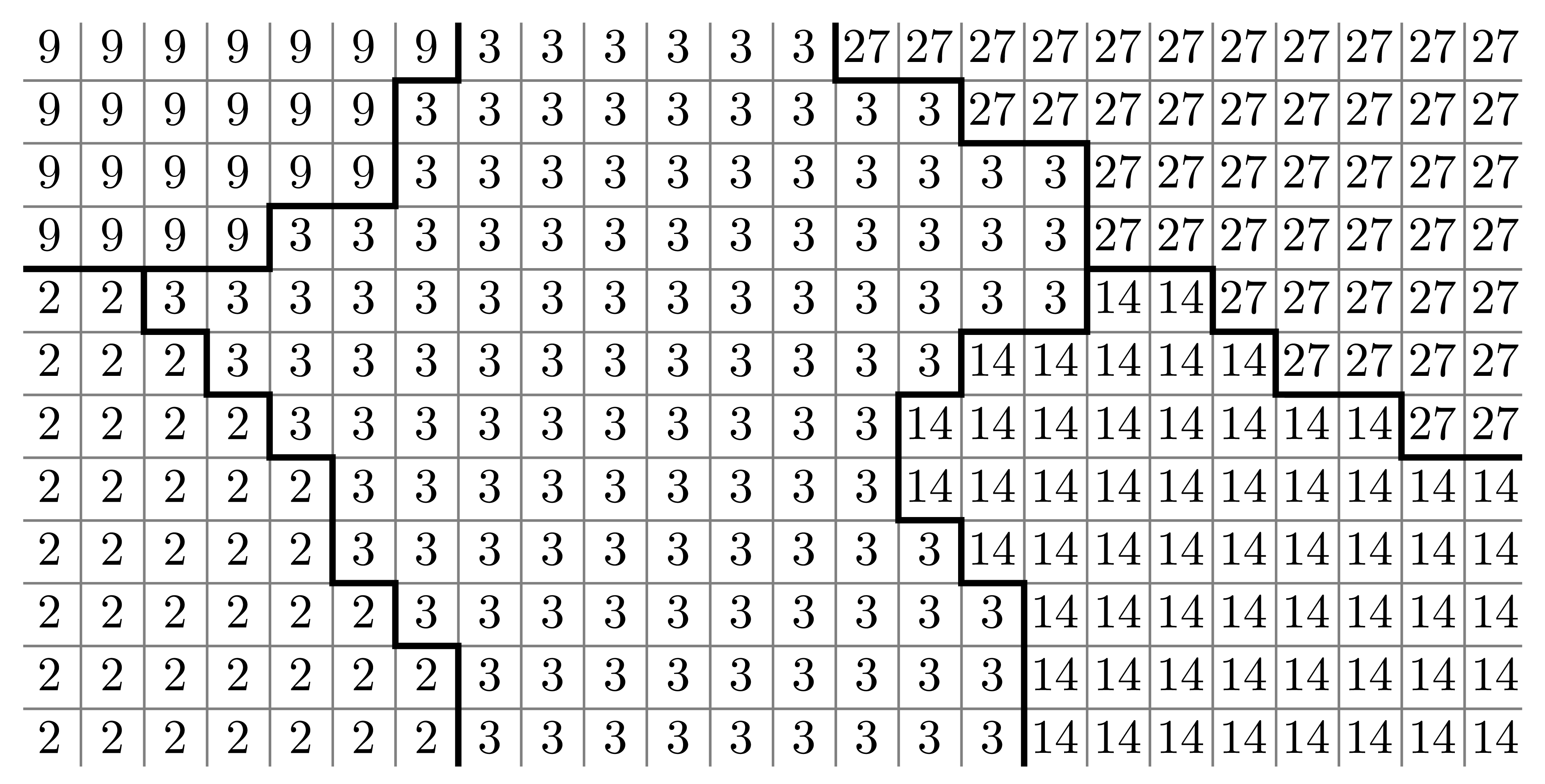
As in the original Ising model, the Monte Carlo Potts algorithm is based on a division of the analysis domain into a grid of N lattice sites. Each lattice site i is given an index si and all sites with a common index belong to the same grain. A schematic representation of a grain structure is shown in Figure 2. Additional parameters can be assigned to each lattice site, containing information on for example crystallographic orientation and dislocation density, characterizing the physical state of the site.
The total energy E of the analysis domain under consideration is calculated from
The evolution of the grain microstructure is now obtained by employing a Monte Carlo sampling of lattice states. A lattice site is chosen at random and a change in the spin state of the site to another of Q possible spins is suggested after which the corresponding change in energy ΔE, due to the changed spin, is calculated from Equation (18). On the basis of ΔE, the suggested spin change is accepted or rejected. A single Monte Carlo step (MCS) involves a total of N spin change attempts. One formulation of the algorithm is obtained by considering lattice sites in pairs and switching the spin states between these sites, leading to Kawasaki dynamics where the volume fraction of each spin is conserved. Non-conserved spin—or Glauber—dynamics, is achieved by considering lattice sites individually and suggesting a new spin at each site [12].
Consistent with the Monte Carlo approach, the switch of a spin state is accepted or rejected on account of a switching probability wswitch (ΔE). As a switch is suggested, a random number ξ ∈ [0, 1] is generated and the switch is accepted if ξ ≤ wswitch (ΔE), otherwise it is rejected. One common choice for the switching probability is the symmetric function
An alternative to Equation (19) is a Metropolis sampling function as discussed in [12].
The morphology of the simulated grain microstructure will be influenced by the underlying lattice onto which the grain structure is mapped. The lattice structure will be represented in the results, giving an undesired faceting of the modeled grain boundaries. This may even influence the grain boundary kinetics as the progress of recrystallization can be slowed down or stopped prematurely. Different remedies for this pathology have been suggested. By one approach, the number of neighbor samplings done for each site is increased, usually by considering an extended set of neighboring sites and not only the nearest sites. A second option is to consider other lattice arrays such as changing from a square to a triangular lattice. A third alternative is to set the simulation temperature Ts > 0 which will serrate the boundaries and by a properly chosen value result in equiaxed grains and correct recrystallization kinetics.
Lacking physical length and time scales, the results from Monte Carlo Potts simulations can be compared to experimental results by different approaches. One option is to relate the length and time scales of the simulation to their physical counterparts and perform a matching of simulated and experimental results. By this method, a real microstructure is mapped onto the simulation lattice, resulting in a matching length scale. In the next step, the simulation is executed until a certain microstructure is achieved that is comparable (statistically) to one obtained from experiments. The simulation time can then be calibrated against the physical time required to reach the same microstructure. This approach is taken in [80]. Alternatively, the parameters of the Monte Carlo Potts model can be interpreted in terms of physical quantities as in [81], giving correct units to the simulation results. The recrystallization kinetics obtained from Monte Carlo Potts simulations are in [35,36,82] shown to agree relatively well with classical KJMA theory.
Although other approaches to grain-scale modeling of recrystallization have appeared, Monte Carlo Potts models of the recrystallization process are still frequently used. The algorithm is versatile and flexible enough to represent many different physical features and processes. The numerical implementation is straight-forward and decent computational efficiency can be achieved, especially since the algorithm is very suitable for parallelization. Less attractive qualities of the algorithm is the influence of the underlying lattice and the lack of physical length and time scales, although remedies for this have been suggested as mentioned previously.
Monte Carlo Potts models have been used in a vast number of studies on aspects of recrystallization. Some have already been mentioned and others include for example [83] where the kinetics of the formulation is studied and the series of papers [82,84,85] where homogeneous and heterogeneous nucleation and particle pinning effects are studied. Dynamic recrystallization is the topic in [86] and the influence of dynamic recovery and deformation temperature on recrystallization is studied in [35,87]. Special grain shapes are studied in [88] and three-dimensional recrystallization simulations are performed in [36]. Note that these are only a few of the published works on Monte Carlo Potts modeling of recrystallization and many more exist.
6. Cellular Automata
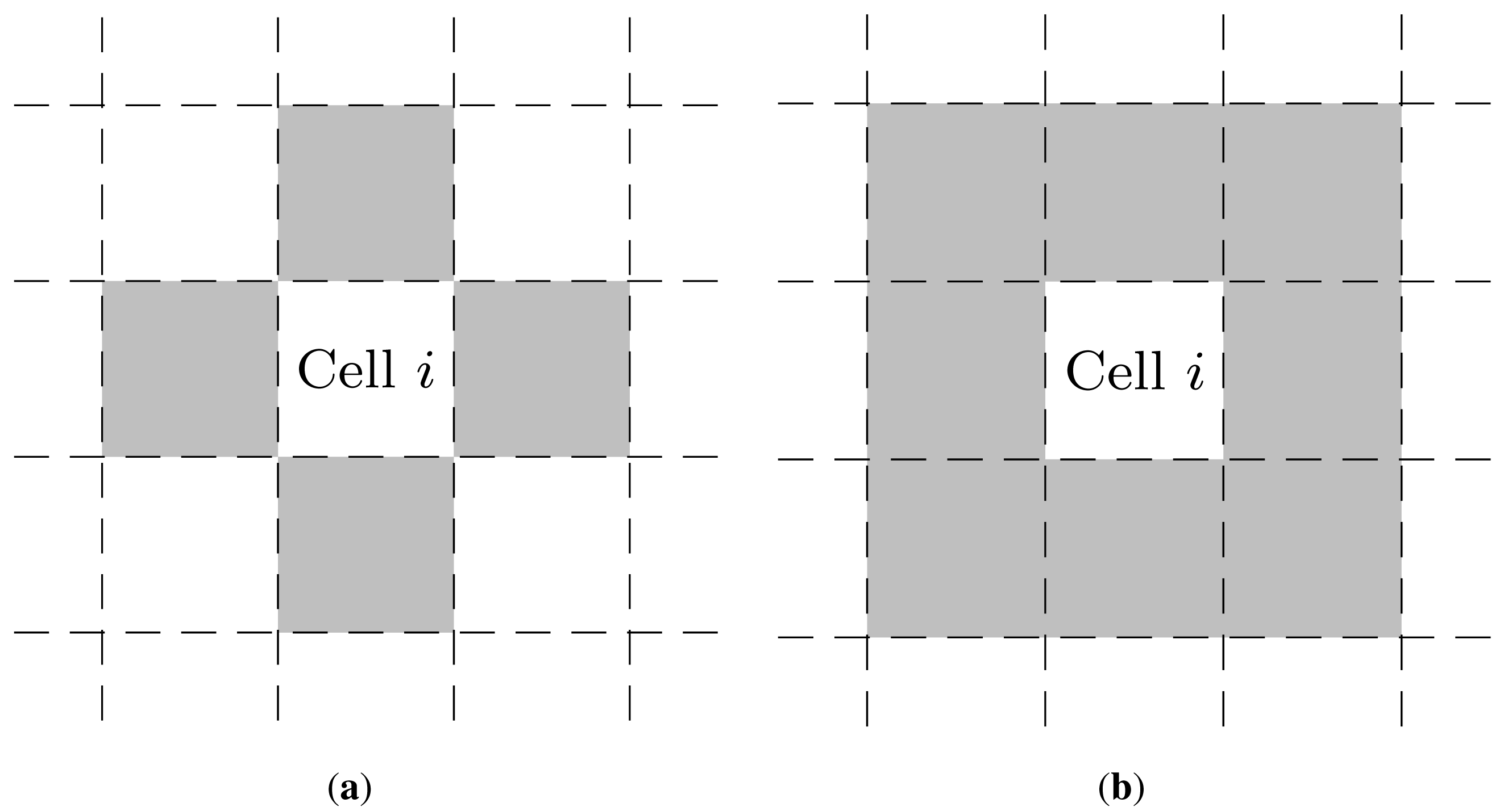
Cellular automata are defined on two- or three-dimensional analysis domains and allow for simulation of both spatial and temporal evolution of microstructures. The analysis domain is partitioned into a grid of sub-regions, the cells. The grid is most often defined as regularly spaced although irregular, or random grid, cellular automata have been employed in [89]. To each cell is assigned a set of state variables which define the physical state represented by the cell, e.g., if it represents recrystallized material or not. In each simulation step, which can be regarded as a time step, a neighborhood of each cell is identified, cf. Figure 3. This might be the nearest neighbor cells or extending further out to include first- and second nearest neighbors or more. The type of neighborhood can be allowed to change between cells and between solution steps. State switching rules are defined to determine the updated state of each cell based on the cell's previous state and the states of the cells in the neighborhood. These switching rules can be taken as deterministic or probabilistic, based on some probability criterion [90]. Discrete solution (time) steps are taken during which the updated states of all cells are calculated, but no cell state is actually changed until the end of the solution step when the states of all cells are updated simultaneously. The time step need not be fixed, but can be allowed to vary. Since the updated cell states are based on the information from a local neighborhood, only small amounts of information have to be passed between cells during state update and hence the cellular automaton algorithm is very amenable for efficient parallelization, providing excellent scalability. Another way to increase the computational efficiency is to only consider boundary cells when performing the cell state update. Since the number of boundary cells is a smaller subset of the total number of cells, a significant gain in computational time is to be made by this approach.
Considering recrystallization, the cell state variables may include the dislocation density, crystallographic orientation and some identification flags, indicating to which grain the cell belongs and if the cell represents recrystallized material or not. If the identification flag of the current cell and any cell in the neighborhood are different, then the current cell is at a grain boundary.
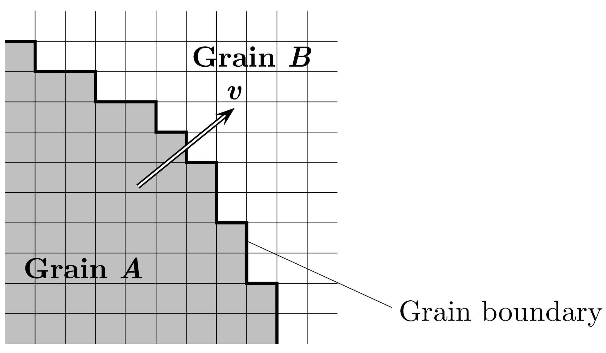
At the beginning of the simulation, state variables are given values to define the initial microstructure. The initial state can be obtained through simulations, e.g., based on crystal plasticity simulations [91], or on experimentally measured data from physical samples. The grain microstructure is defined by cells belonging to different grains and a schematic illustration of a grain boundary representation in the cellular automaton is shown in Figure 4.
The cellular automaton domain can be analyzed under any combination of boundary conditions along the edges including periodic, symmetric and mirror boundary conditions.
Grain boundary kinetics are conveniently described in the cellular automaton using Equations (6)–(11) and state variables such as dislocation density can be updated in each time step by employing evolution laws on rate form [19].
Considering a fixed grid cellular automaton, the typical cell size lc would be the distance traveled by a migrating grain boundary during a single time step. With the grain boundary velocity given by Equation (6), this would allow the global time step Δt to be calculated as
However, since the driving pressure p and possibly also the mobility m are local quantities that varies throughout the microstructure, this approach is not feasible. An alternative approach is to introduce probabilistic cell state switching rules like in the “hybrid” model introduced in [3,92]. This can be achieved by considering a local switching probability wswitch as was defined in Equation (19) for the Monte Carlo Potts method. For each cell having an approaching grain boundary in its neighborhood, this probability is calculated as
If continuous rather than site-saturated nucleation is considered, nucleation of new grains can be incorporated into the cellular automaton algorithm by employing an evolution law for the nucleation on rate form as in Equation (5). In this way the number of nuclei to appear during a time step can be calculated. Positioning of the nuclei can then be performed randomly at suitable sites, primarily along grain boundaries, or deterministic at sites that fulfill some nucleation criterion, e.g., in terms of a critical dislocation density as discussed in relation to Equation (4). Preferably, cell sites with the highest dislocation density are consumed first, corresponding to the recrystallization process working to lower the stored energy. Viewing the cellular automaton as a representative volume element, quantities such as macroscopic flow stress can be obtained by some homogenization procedure as employed in [19].
Cellular automata for recrystallization modeling are discussed in the review paper [93] and also in [12].
As discussed in [12,94], the shape of the grains in the cellular automaton will be influenced by the grid discretization and certainly by the choice of cell neighborhood, cf. Figure 3. Simulation of recrystallization, using a deterministic cellular automaton, was performed in [95] where the influence of the selected cell neighborhood is seen to control the shape of the recrystallized grains. Issues as these have resulted in a number of studies on how tho represent surfaces and curvature on grids like the ones employed in cellular automata. Calculation of the local curvature is also important in establishing the grain boundary energy γ, appearing in Equation (7). One approach to estimate the local boundary curvature is by use of kink-templates as formulated in [96], also used in [19,38,97]. By this approach, an expanded cell neighborhood is considered—the “template”—and the curvature is estimated based on the number of cells belonging to the grain in question and the number of cells that would constitute a planar interface in the template region.
The cellular automaton algorithm offers attractive possibilities in simulation of microstructure processes, one advantage being high spatial resolution. In addition, unlike many other numerical solution schemes and especially those based on continuous fields, cellular automata provide excellent scalability for computer code parallelization, giving computational efficiency Since the microstructure is fully represented, local effects are considered unlike in phenomenological models. Discrete, rather than homogenized, processes are modeled. Cellular automata are also versatile tools in computational materials science since arbitrary constitutive relations and cell state switching rules can be used. They are also capable of replicating the recrystallization kinetics obtained from the KJMA model, as shown in [19]. A disadvantage of the method, pertaining to recrystallization modeling, is the inability of cellular automata to trace texture evolution due to macroscopic deformation.
Additional examples from the vast number of studies where cellular automata have been used in modeling of recrystallization can be found in [98] and [37] where dynamic recrystallization is studied and in [99] in relation to multi-stage hot deformation. In addition, Zener pinning is studied in [50], irregular cellular automata is used in simulation of dynamic recrystallization in [100] and recrystallization during hot rolling is modeled in [46]. Many additional examples exist.
7. Phase Field Models
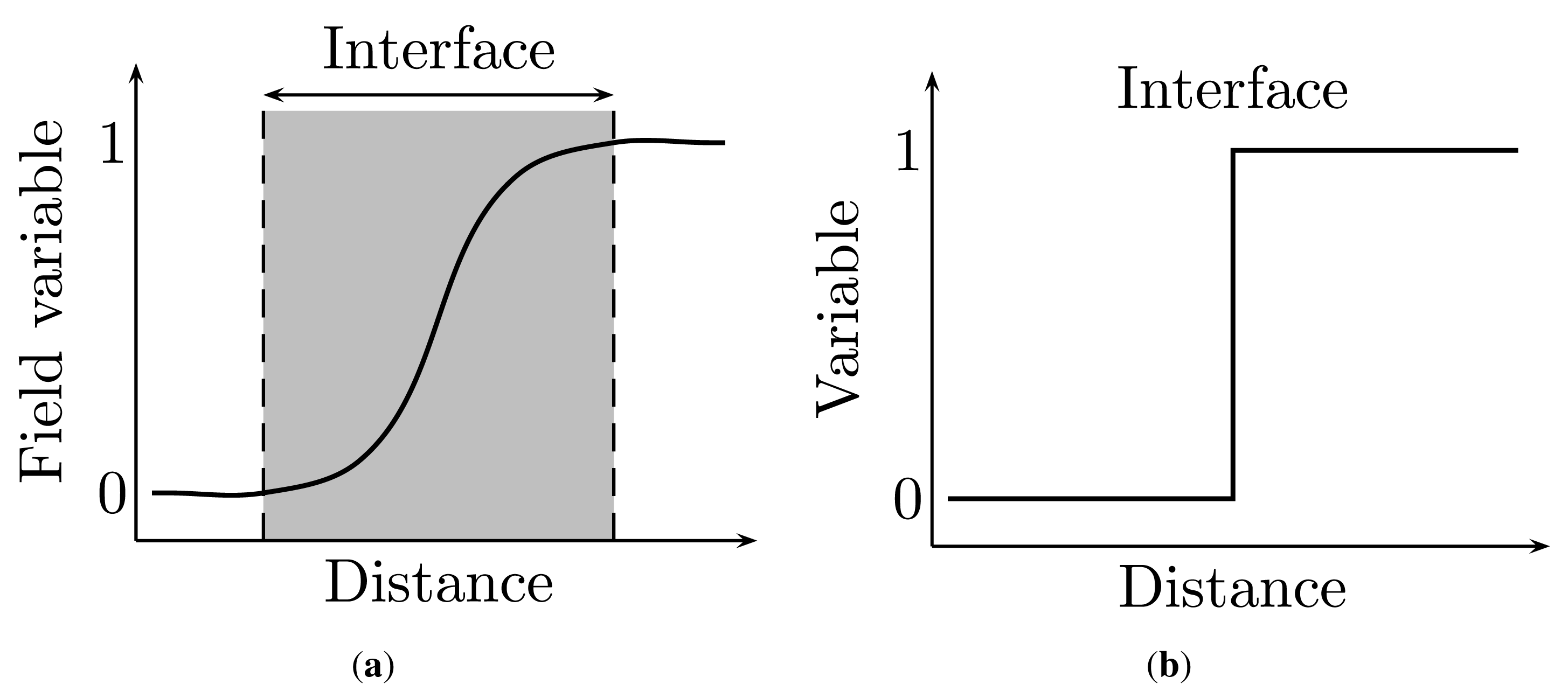
In phase field models of recrystallization, the grain microstructure is described by phase field variables. These are functions that are continuous in space and a distinction is made between conserved and non-conserved variables. A conserved variable is typically a measure of the local composition whereas a non-conserved variable contains information on the local structure and could represent for example the crystallographic orientation. Within a single grain, a phase field variable maintains a nearly constant value that correspond to the properties of that grain. Grain boundaries are represented as interfaces where the value of the phase field variable gradually varies between the values in the neighboring grains on opposing sides of the grain boundary. Grain boundaries are hence described as diffuse transition regions of the phase field variables in contrast to sharp interface models where jump discontinuities in quantities such as the energy occurs. This is schematically illustrated in Figure 5. The sharp interface description can be retrieved from the phase field formulation by considering the sharp interface limit of the phase field model through asymptotic expansion, whereby the width of the diffuse interface tends to zero.
As a consequence of the diffuse interface formulation, there is no need to explicitly trace the location of interfaces as in sharp interface models. This allows arbitrary grain morphologies to be represented without any assumptions on the grain shapes. The evolution of phase field variables in time is calculated from a set of partial differential equations that are solved numerically.
The governing equations for a system of two coexisting phases described by a non-conserved, continuous, phase field ϕ(x, t), where x is the spatial position of a material point, was first presented in [101]. In such models, the single phase field will have a value of 0 in one phase and 1 in the other. Often applied to the process of solidification of melts, this formulation could be interpreted as ϕ = 0 in the liquid and ϕ = 1 in the solid phase, respectively. The single-phase field representation was later elaborated to consider multiphase systems in [102,103]. Such a system, containing a total of N coexisting phases, is described by employing N phase field variables—or order parameters—ηk where k = 1…N, corresponding to the local fractions of each phase. The phase fields are thus subject to the condition
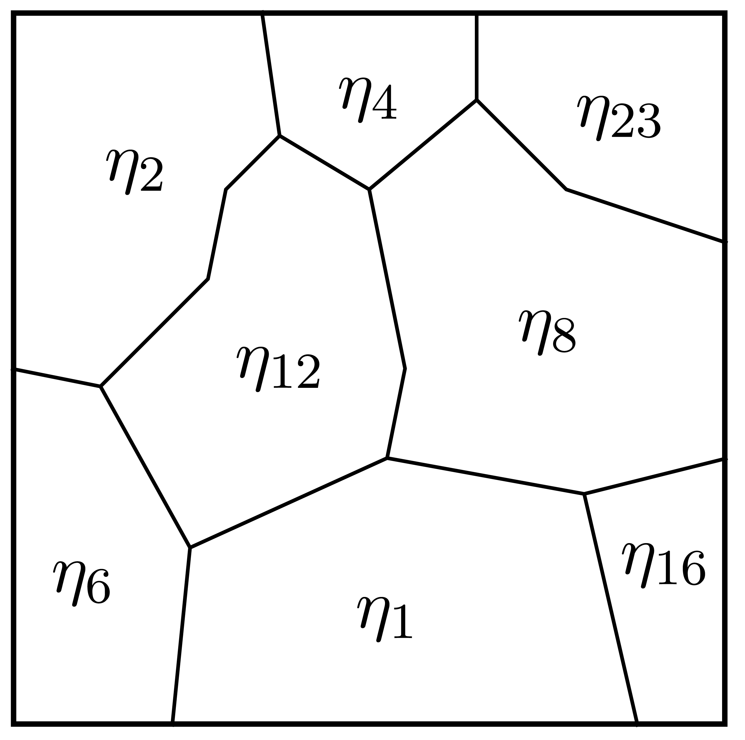
Figure 6 schematically illustrates a grain structure represented by the orientation parameters ηk, corresponding to individual grains. In a grain indexed by i it holds that ηi = 1 while all other parameters ηk≠i = 0. Grain boundaries will be represented by intermediate combinations of the ηk parameters.
In addition to the ηk-variables, also a set of n conserved variables ci, i = 1…n, could be introduced. The ci-variables could be used to represent for example a conserved concentration of solute atoms as in [51] where solute drag is studied (with n = 1).
As discussed initially, the driving force for recrystallization is a minimization of the energy of the system. This energy can be viewed to consist of different components related to interfacial energy, bulk energy, elastic energy and so on. In a phase field setting, the energy is established as a functional of the phase field variables and their gradients in contrast to standard thermodynamics where a homogeneous distribution of the properties is assumed. The approach for systems with diffuse interfaces and heterogeneous properties was first established in [105]. Phase field models of microstructure evolution differ mainly in the treatment of different components in the energy functional. Following [102,106], and as discussed in [107,108], the energy functional of a multiphase system under constant temperature can be generally written as
Evolution laws for the orientation variables ηk and the conserved variables ci are established from the energy functional in Equation (24). This is achieved by using the time-dependent Ginzburg–Landau or Allen–Cahn Equation [109] for the non-conserved variables ηk and a Cahn–Hilliard Equation [110] for the conserved variables ci. This results in evolution equations on the form
The evolution laws in Equation (25) can be solved using some numerical scheme like finite differences, finite elements or by spectral algorithms. As interfaces have to be resolved, a relatively fine computational grid has to be used, adding to the computational effort. Employing grid adaptivity may help in reducing this effort. When microstructures containing a large number of grains are considered, this may however prove impractical.
Phase field models have during the last two decades been employed in simulations of a number of different microstructure processes. Arbitrary microstructure geometries such as grains can be represented without the need of explicitly tracing interfaces. Phase field models also provide the possibility to consider a wide array of microstructure processes based on thermodynamic formulations. The computational effort involved in simulating an evolving microstructure using phase fields is quite significant. Remedies such as adaptivity of the discretization grid can reduce the computational time, as can code parallelization although not as efficiently as with discrete methods such as Monte Carlo Potts formulations or cellular automata. Phase field models are capable of tracing arbitrary grain interface geometries and their evolution although the method is less applicable in studies of texture evolution.
Phase field modeling in materials science in general is reviewed in [107,108,111] and with particular focus on recrystallization in [4]. The kinetics of the KJMA model for evolution of microstructures are compared to phase field models in [112] with acceptable agreement. Differences are explained by the assumptions made in the KJMA model. Phase field and Monte Carlo Potts models of grain coarsening are compared in [113]. Additional examples of studies where grain growth is modeled using phase field simulations can be found in [51,104] where, in the latter paper, solute drag is included. In addition, three-dimensional grain growth is studied in [114] and grain growth in the presence of second-phase particles in [52]. Curvature-driven grain growth in two and three dimensions is modeled in [115] and three-dimensional grain growth in a particle-containing material in [54]. The influence of stored energy on the recrystallization kinetics is treated in [116]. SRX is studied in a model combining phase field and crystal plasticity models in [117]. Phase field studies on recrystallization where also nucleation is considered, are presented in [118,119] and specifically for an AZ31 Mg alloy in [120].
8. Vertex Models
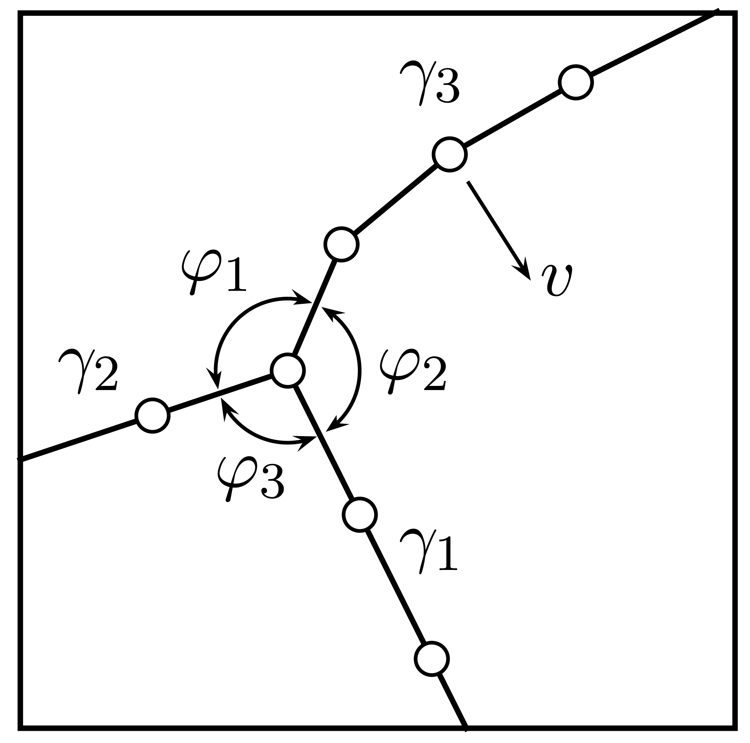
Vertex, or front tracking, models for simulation of grain growth have been established by a number of authors, e.g., in [121–126]. In most models, a two-dimensional grain structure is considered and its geometry is represented by line segments—the grain boundaries—connected at nodes or vertices which are positioned at triple (in 2D) or quadruple (in 3D) junctions and possibly also at intermediate positions along the grain boundary, cf. Figure 7. The grain structure is thus defined by the positions x of the nodes and their velocities υ, represented as vectors.
In vertex models it is common to assume the triple or quadruple junctions to be in equilibrium, although the discussion in [127] indicates that relaxation of this assumption only has a minor impact on the simulation results. With the notation shown in Figure 7, where γi are the grain boundary energies, the equilibrium separation angles φi can be found from the relation
Grain boundary migration is considered as a dissipative process and based on a grain boundary segment of length a between two vertices, the grain boundary energy is obtained from
The summations in Equation (30) are performed over the entire domain but couplings are only made between individual vertices and their neighbors whereby Equation (31) gives the local result for each vertex. More details on these derivations can be found in [123,125]. Note that special measures have to be taken for vertices lying on boundaries between junctions to determine when they begin to move, as discussed in [125]. Simplifications to the solution of Equation (31) are suggested in [123] to increase the computational efficiency of the model. The latter model is based on nodes being placed solely at triple junctions and not at intermediate positions. This methodology is also employed in [1,128]. The merit of this approach is reduced computational cost, however at the expense of grain boundaries being simplified as straight segments between the junctions. This will influence the equilibrium configuration at triple junctions where the three connecting boundaries ideally should be separated by 120° angles, cf. Figure 7. Using straight grain boundaries will also alter the boundary migration rates. This is considered to be the main cause of mismatch in comparing recrystallization kinetics obtained from a vertex model to that of a Monte Carlo Potts model in [123]. Better agreement with Monte Carlo Potts kinetics is found in [125] where also intermediate vertices are introduced.
During simulation, the topology of the microstructure changes and transformation rules have to be established. Considering the two-dimensional case, and if only nodes at triple junctions are employed, the transformation rules involve recombination of junctions and removal of three-sided grains below a certain size. These processes as often denoted as T1 and T2 transformations. Additional transformation rules are included if also intermediate vertices are introduced [125].
The velocities of the vertices are obtained from Equation (31), allowing the new positions of the vertices to be calculated as
Vertex, or front tracking, models are mentioned in the reviews [2,4] and grain growth in thin films is studied using a vertex method in [129] where also strain energy effects are included. The method has also been employed in [130], considering Zener pinning effects. Vertex models have mostly been used in two-dimensional simulations of recrystallization processes—as in the publications so far mentioned—mainly due to the formulation becoming significantly more involved in three dimensions where tessellation of surfaces has to be performed and where the number of topological changes increase. Three-dimensional simulations of migrating grain boundaries interacting with rigid particles are, however, shown in [48]. The surfaces of the grain boundaries are represented by a mesh of triangular elements and the authors note that the simulation results depend on the mesh quality and can become biased as the surface mesh is distorted. Three-dimensional grain growth is also studied in [131] using a vertex model.
Vertex models are not as widely used in recrystallization modeling as for example Monte Carlo Potts models and cellular automata, but attractive features of the method include a physical time scale [125] and the possibility to better resolve grain boundary curvature.
9. Level Set Models
Use of level set formulations to model recrystallization is, at least compared to cellular automata and Monte Carlo Potts models, a relatively recent development. The central concept of the method is to trace the position of a moving interface Γ (t) with time. A continuous function ϕ(x, t) is introduced to represent the interface with dependence on space and time. The interface Γ (t) is represented as the zero level set of the function ϕ(x, t) and by convention it then holds that
The motion of the interface Γ (t) is given by
Considering a grain microstructure with several grains, the level set formulation is expanded so that each grain i is given an independent level set function ϕi (x, t). New grains that appear due to nucleation are added by introducing additional level set functions. Each level set function is allowed to evolve separately during a time step in the solution. In order to avoid overlapping domains or voids between interfaces, a correction or smoothing step is employed at the end of each time step to restore the topology. As introduced in [133], this can be achieved by establishing corrected level set functions which can be calculated from
The level set representation of grain boundaries allows convenient treatment of boundary curvature since it is obtained directly from the level set functions. The unit normal to the boundary is given by
To some extent, the evolution of the level set method resembles that of the phase field method, beginning with systems of two separate phases. The level set formulation was introduced in [134] and was later used in [135] to study two-phase incompressible flow. The model was also elaborated to consider interfaces with multiple junctions in [133,136]. In a series of papers by the same group of authors, level set models are used in both two- and three-dimensional finite element models to simulate recrystallization and grain growth [132,137–139]. Coupling of a crystal plasticity finite element model with a level set formulation of recrystallization is presented in [140]. A level set approach is also taken in [141,142] where a finite difference scheme is used on fixed grids, also in both two and three dimensions. In these publications, some simplifications are made, for example in terms of the boundary mobilities and the boundary energies not being dependent on the misorientation between adjacent grains.
As with the phase field formulation, the level set method also allows a direct representation of interfaces and curvature that is not possible in Monte Carlo Potts models and cellular automata. There is also no need to explicitly treat the interface discretization as is required in vertex models. Fundamental topological changes of the grain microstructure such as the T1 and T2 transformations that requires special treatment in the vertex method, as discussed in Section 8, are captured by the level set method without additional considerations. A disadvantage of the level set method is its inability to trace textural evolution. A possible remedy for this might be a combination of crystal plasticity and level set formulations. In [132], the recrystallization kinetics of the level set formulation is shown to agree with classical KJMA theory. A local level set formulation is established in [143] to reduce computation time. As discussed in relation to the phase field method, also level set models need to resolve the sharp interfaces constituting the grain boundaries. This poses the need for adaptivity of the element mesh or solution grid, which of course adds to the computation time.
10. Concluding Remarks
This paper reviews the main methodologies in modeling and simulation of recrystallization. Analytical and empirical results as well as numerical methods are considered. Numerical formulations that are discussed include continuum mechanical models and discrete approaches such as Monte Carlo Potts models and cellular automata as well as vertex, phase field and level set models.
Both Monte Carlo Potts models and cellular automata are well established in computational materials science and have been widely used in the study of recrystallization phenomenon. They are relatively easily implemented and can be used to capture many aspects of the microstructure physics during recrystallization. High computational efficiency can be obtained using these methods since the discrete nature of the algorithms is well suited for parallelization. Limitations lie mainly in the dependence on the underlying solution grid, representation of grain boundary curvature and in the interpretation of simulation length and time scales.
The vertex, or front tracking, method is a more recent contribution that has been used to some extent in recrystallization simulations. The method is more involved to implement and more computationally demanding. Grain boundaries can be better represented than in Monte Carlo Potts models and cellular automata, but the numerical scheme has to be employed with special consideration regarding topological changes in the microstructure. To include curved grain boundaries, vertices need to be placed between junctions, involving additional calculation steps.
Phase field formulations are being increasingly employed in computational materials science. Most phase field studies on recrystallization have been conducted on grain growth, avoiding the nucleation stage. Such investigations have, however, begun to appear and the development will certainly continue. Phase field simulations are more computationally intensive than for example Monte Carlo Potts models and cellular automata and are also less amenable for parallelization. Still, the representation of surfaces is better and there is no need for explicit tracing of interfaces as in the vertex method. To properly resolve distinct interfaces, adaptivity of the solution mesh or grid is often employed, adding to the computational load.
Level set models of recrystallization are still relatively few although the method has many appealing traits. As in the phase field method, grain boundary migration can be directly established without tracing interfaces. Boundary curvature is conveniently obtained and many aspects of grain structure evolution, such as appearance and disappearance of grains, can be included. As with the phase field method, also the level set representation of narrow interfaces require a fine computational grid or mesh. Again, adaptivity can be used at the expense of extra computation time.
Applying to all of the numerical methods discussed herein, they become computationally more expensive as three-dimensional models and larger numbers of grains are considered.
All of the methods discussed have both merits and disadvantages and selecting what method to use is largely a matter of the physics and complexity of the problem at hand, of available computational resources and of course also of personal preference.


References
- Humphreys, F. Modelling mechanisms and microstructures of recrystallisation. Mater. Sci. Technol. 1992, 8, 135–144. [Google Scholar]
- Rollett, A. Overview of modeling and simulation of recrystallization. Prog. Mater. Sci. 1997, 42, 79–99. [Google Scholar]
- Rollett, A.; Raabe, D. A hybrid model for mesoscopic simulation of recrystallization. Comput. Mater. Sci. 2001, 21, 69–78. [Google Scholar]
- Miodownik, M. A review of microstructural computer models used to simulate grain growth and recrystallisation in aluminium alloys. J. Light Met. 2002, 2, 125–135. [Google Scholar]
- Doherty, R.; Hughes, D.; Humphreys, F.; Jonas, J.; Jensen, D.J.; Kassner, M.; King, W.; McNelley, T.; McQueen, H.; Rollett, A. Current issues in recrystallization: A review. Mater. Sci. Eng. A 1997, 238, 219–274. [Google Scholar]
- Humphreys, F.; Hatherly, M. Recrystallization and Related Annealing Phenomena, 2nd ed.; Pergamon: New York, NY, USA, 2004. [Google Scholar]
- Gourdet, S.; Montheillet, F. An experimental study of the recrystallization mechanism during hot deformation of aluminium. Mater. Sci. Eng. A 2000, 283, 274–288. [Google Scholar]
- Mazurina, I.; Sakai, T.; Miura, H.; Sitdikov, O.; Kaibyshev, R. Effect of deformation temperature on microstructure evolution in aluminum alloy 2219 during hot ECAP. Mater. Sci. Eng. A 2008, 486, 662–671. [Google Scholar]
- Sakai, T.; Miura, H.; Yang, X. Ultrafine grain formation in face centered cubic metals during severe plastic deformation. Mater. Sci. Eng. A 2008, 499, 2–6. [Google Scholar]
- Rossard, C.; Blain, P. Evolution de la structure de l'acier sous l'effet de la dèformation plastique á chaud. Mem. Sci. Rev. Metall. 1959, 56, 285–300. [Google Scholar]
- Blaz, L.; Sakai, T.; Jonas, J. Effect of initial grain-size on dynamic recrystallization of copper. Metall. Sci. 1983, 17, 609–616. [Google Scholar]
- Janssens, K.; Raabe, D.; Kozeschnik, E.; Miodownik, M.; Nestler, B. Computational Materials Engineering; Elsevier Academic Press: London, UK, 2007. [Google Scholar]
- Gottstein, G.; Schvindlerman, L. Grain Boundary Migration in Metals, 2nd ed.; CRC Press: Boca Raton, FL, USA, 2010. [Google Scholar]
- Kolmogorov, A. Statistical theory of crystallization of metals (in Russian). Bull. Acad. Sci. USSR Ser. Math. 1937, 1, 355–359. [Google Scholar]
- Johnson, W.; Mehl, R. Reaction kinetics in processes of nucleation and growth. Trans. Am. Inst. Min. Metall. Eng. 1939, 135, 416–458. [Google Scholar]
- Avrami, M. Kinetics of phase change, I. General theory. J. Chem. Phys. 1939, 7, 1103–1112. [Google Scholar]
- Avrami, M. Kinetics of phase change, II. Transformation-time relations for random distribution of nuclei. J. Chem. Phys. 1940, 8, 212–224. [Google Scholar]
- Avrami, M. Kinetics of phase change, III. Granulation, phase change and microstructure. J. Chem. Phys. 1941, 9, 177–184. [Google Scholar]
- Hallberg, H.; Wallin, M.; Ristinmaa, M. Modeling of continuous dynamic recrystallization in pure Cu using a probabilistic cellular automaton. Comput. Mater. Sci. 2010, 49, 25–34. [Google Scholar]
- Furu, T.; Marthinsen, K.; Nes, E. Modelling recrystallization. Mater. Sci. Technol. 1990, 6, 1093–1102. [Google Scholar]
- Todinov, M. On some limitations of the Johnson-Mehl-Avrami-Kolmogorov equation. Acta Mater. 2000, 48, 4217–4224. [Google Scholar]
- Farjas, J.; Roura, P. Modification of the Kolmogorov-Johnson-Mehl-Avrami rate equation for non-isothermal experiments and its analytical solution. Acta Mater. 2006, 54, 5573–5579. [Google Scholar]
- Shercliff, H.; Lovatt, A.; Jensen, D.J.; Beynon, J. Modelling of microstructure evolution in hot deformation. Philos. Trans. R. Soc. Lond. A 1999, 357, 1621–1643. [Google Scholar]
- Belyakov, A.; Miura, H.; Sakai, T. Dynamic recrystallization under warm deformation of a 304 type austenitic stainless steel. Mater. Sci. Eng. A 1998, 255, 139–147. [Google Scholar]
- Gao, W.; Belyakov, A.; Miura, H.; Sakai, T. Dynamic recrystallization of copper polycrystals with different purities. Mater. Sci. Eng. A 1999, 285, 233–239. [Google Scholar]
- Wusatowska-Sarnek, A.; Miura, H.; Sakai, T. Nucleation and microtexture development under dynamic recrystallization of copper. Mater. Sci. Eng. A 2002, 323, 177–186. [Google Scholar]
- Miura, H.; Ozama, M.; Mogawa, R.; Sakai, T. Strain-rate effect on dynamic recrystallization at grain boundary in Cu alloy bicrystal. Scr. Mater. 2003, 48, 1501–1505. [Google Scholar]
- Goetz, R. Particle stimulated nucleation during dynamic recrystallization using a cellular automata model. Scr. Mater. 2005, 52, 851–856. [Google Scholar]
- Roberts, W.; Ahlbom, B. A nucleation criterion for dynamic recrystallization during hot working. Acta Metall. 1978, 26, 801–813. [Google Scholar]
- Peczak, P.; Luton, M. The effect of nucleation models on dynamic recrystallization. I. Homogeneous stored energy distribution. Philos. Mag. B 1993, 68, 115–144. [Google Scholar]
- Peczak, P.; Luton, M. The effect of nucleation models on dynamic recrystallization. II. Heterogeneous stored-energy distribution. Philos. Mag. B 1993, 70, 817–849. [Google Scholar]
- Roucoules, C.; Pietrzyk, M.; Hodgson, P. Analysis of work hardening and recrystallization during the hot working of steel using a statistically based internal variable model. Mater. Sci. Eng. A 2003, 339, 1–9. [Google Scholar]
- Bernard, P.; Bag, B.; Huang, K.; Logé, R.E. A two-site mean field model of discontinuous dynamic recrystallization. Mater. Sci. Eng. A 2011, 528, 7357–7367. [Google Scholar]
- Bailey, J.; Hirsch, P. The recrystallization process in some polycrystalline metals. Proc. R. Soc. Lond. A 1962, 267, 11–30. [Google Scholar]
- Peczak, P. A Monte Carlo study of the influence of deformation temperature on dynamic recrystallization. Acta Metall. Mater. 1995, 43, 1279–1291. [Google Scholar]
- Ivasishin, O.; Vasiliev, S.S.N.; Semiatin, S. A 3-D Monte-Carlo (Potts) model for recrystallization and grain growth in polycrystalline materials. Mater. Sci. Eng. A 2006, 433, 216–232. [Google Scholar]
- Ding, R.; Guo, Z. Coupled quantitative simulation of microstructural evolution and plastic flow during dynamic recrystallization. Acta Mater. 2001, 49, 3163–3175. [Google Scholar]
- Zheng, C.; Li, N.X.D.; Li, Y. Mesoscopic modeling of austenite static recrystallization in a low carbon steel using a coupled simulation method. Comput. Mater. Sci. 2009, 45, 568–575. [Google Scholar]
- Burke, J.; Turnbull, D. Recrystallization and grain growth. Prog. Met. Phys. 1952, 3, 220–292. [Google Scholar]
- Read, W.; Shockley, W. Dislocation models of crystal grain boundaries. Phys. Rev. 1950, 78, 275–289. [Google Scholar]
- Wolf, D. A Read-Shockley model for high-angle grain boundaries. Scr. Metall. 1989, 23, 1713–1718. [Google Scholar]
- Smith, C. Grains, phases and interfaces: An interpretation of microstructure. Trans. Am. Inst. Min. Metall. Eng. 1948, 175, 15–51. [Google Scholar]
- Louat, N. The resistance to normal grain growth from a dispersion of spherical particles. Acta Metall. Mater. 1982, 30, 1291–1294. [Google Scholar]
- Nes, E.; Ryum, N.; Hunderi, O. On the Zener drag. Acta Metall. Mater. 1985, 33, 11–22. [Google Scholar]
- Hunderi, O.; Nes, E.; Ryum, N. On the Zener drag—Addendum. Acta Metall. Mater. 1989, 37, 129–133. [Google Scholar]
- Zheng, C.; Li, N.X.D.; Li, Y. Microstructure prediction of the austenite recrystallization during multi-pass steel strip hot rolling: A cellular automaton modeling. Comput. Mater. Sci. 2008, 44, 507–514. [Google Scholar]
- Mendelev, M.; Srolovitz, D. Impurity effects on grain boundary migration. Model. Simul. Mater. Sci. Eng. 2002, 10, 79–110. [Google Scholar]
- Harun, A.; Holm, E.; Clode, M.; Miodownik, M. On computer simulation methods to model Zener pinning. Acta Mater. 2006, 54, 3261–3273. [Google Scholar]
- Miodownik, M.; Holm, E.; Hassold, G. Highly parallel computer simulations of particle pinning; Zener vindicated. Scr. Mater. 2000, 42, 1173–1177. [Google Scholar]
- Raabe, D.; Hantcherli, L. 2D cellular automaton simulation of the recrystallization texture of an IF sheet steel under consideration of Zener pinning. Comput. Mater. Sci. 2005, 34, 299–313. [Google Scholar]
- Fan, D.; Chen, S.; Chen, L.Q. Computer simulation of grain growth kinetics with solute drag. J. Mater. Res. 1999, 14, 1113–1123. [Google Scholar]
- Moelans, N.; Blanpain, B.; Wollants, P. A phase field model for the simulation of grain growth in materials containing finely dispersed incoherent second-phase particles. Acta Mater. 2005, 53, 1771–1718. [Google Scholar]
- Moelans, N.; Blanpain, B.; Wollants, P. Phase field simulations of grain growth in two-dimensional systems containing finely dispersed second-phase particles. Acta Mater. 2006, 54, 1175–1184. [Google Scholar]
- Suwa, Y.; Saitob, Y.; Onoderac, H. Phase field simulation of grain growth in three dimensional system containing finely dispersed second-phase particles. Scr. Mater. 2006, 55, 407–410. [Google Scholar]
- Humphreys, F. A unified theory of recovery, recrystallization and grain growth, based on stability and growth of cellular microstructures—I. The basic model. Acta Mater. 1997, 45, 4231–4240. [Google Scholar]
- Montheillet, F.; Lurdos, O.; Damamme, G. A grain scale approach for modeling steady-state discontinuous dynamic recrystallization. Acta Mater. 2009, 57, 1602–1612. [Google Scholar]
- May, J.; Höppel, H.; Göken, M. Strain rate sensitivity of ultrafine-grained aluminum processed by severe plastic deformation. Scr. Mater. 2005, 53, 189–194. [Google Scholar]
- Germain, P.; Nguyen, Q.; Suquet, P. Continuum thermodynamics. J. Appl. Mech. 1983, 91, 1010–1020. [Google Scholar]
- Reddy, B.; Martin, J. Internal variable formulations and problems in elastoplasticity: Constitutive and algorithmic aspects. Appl. Mech. Rev. 1994, 47, 429–456. [Google Scholar]
- Hallberg, H.; Wallin, M.; Ristinmaa, M. Modeling of continuous dynamic recrystallization in commercial-purity aluminum. Mater. Sci. Eng. A 2010, 527, 1126–1134. [Google Scholar]
- Sakai, T.; Jonas, J. Dynamic recrystallization: Mechanical and microstructural considerations. Acta Metall. Mater. 1984, 32, 189–209. [Google Scholar]
- Medina, S.; Hernandez, C. Modelling of the dynamic recrystallization of austenite in low alloy and microalloyed steels. Acta Mater. 1996, 44, 165–171. [Google Scholar]
- Busso, E. A continuum theory for dynamic recrystallization with microstructure-related length scales. Int. J. Plast. 1998, 14, 319–353. [Google Scholar]
- Chiesa, M.; Brown, A.; Antoun, B.; Ostien, J.; Regueiro, R.; Bammann, D.; Yang, N. Predicition of Final Material State in Multi-Stage Forging Processes. In Materials Processing and Design: Modeling, Simulation And Applications, Proceedings of the 8th International Conference on Numerical Methods in Industrial Forming Processes (NUMIFORM), Columbus, OH, USA; 2004; pp. 510–515. [Google Scholar]
- Brown, A.; Bammann, D.; Chiesa, M.; Winters, W.; Ortega, A.; Antoun, B.; Yang, N. Modeling Static and Dynamic Recrystallization in FCC Metals. In Anisostropy, Texture, Dislocations and Multiscale Modeling in Finite Plasticity and Viscoplasticity, and Metal Forming, Proceedings of the 12th International Symposium on Plasticity, Halifax, NS, Canada; 2006; pp. 481–583. [Google Scholar]
- Cahn, J. The kinetics of grain boundary nucleated reactions. Acta Metall. Mater. 1956, 4, 449–459. [Google Scholar]
- Sandström, R.; Lagneborg, R. A model for static recrystallization after hot deformation. Acta Metall. Mater. 1975, 23, 481–488. [Google Scholar]
- Jonas, J. Dynamic recrystallization—Scientific curiosity or industrial tool? Mater. Sci. Eng. A 1994, 184, 155–165. [Google Scholar]
- Lin, J.; Liu, Y. A set of unified constitutive equations for modelling microstructure evolution in hot deformation. J. Mater. Process. Technol. 2003, 143–144, 281–285. [Google Scholar]
- Qu, J.; Jin, Q.; Xu, B. Parameter identification for improved viscoplastic model considering dynamic recrystallization. Int. J. Plast. 2005, 21, 1267–1302. [Google Scholar]
- Nes, E. Constitutive laws for steady state deformation of metals, a microstructural model. Scr. Metall. Mater. 1995, 33, 225–231. [Google Scholar]
- Nes, E.; Furu, T. Application of microstructurally based constitutive laws to hot deformation of aluminum alloys. Scr. Metall. Mater. 1995, 33, 87–92. [Google Scholar]
- Sellars, C.; Zhu, Q. Microstructural modelling of aluminium alloys during thermomechanical processing. Mater. Sci. Eng. A 2000, 280, 1–7. [Google Scholar]
- Duan, X.; Sheppard, T. Influence of forming parameters on static recrystallization behaviour during hot rolling aluminium alloy 5083. Model. Simul. Mater. Sci. Eng. 2002, 10, 363–380. [Google Scholar]
- Ahmed, H.; Wells, M.; Maijer, D.; Howes, B.; van der Winden, M. Modelling of microstructure evolution during hot rolling of AA5083 using an internal state variable approach integrated into an FE model. Mater. Sci. Eng. A 2005, 390, 278–290. [Google Scholar]
- Potts, R. Some generalized order-disorder transformations. Proc. Camb. Philos. Soc. 1952, 48, 106–109. [Google Scholar]
- Anderson, M.; Srolovitz, D.; Grest, G.; Sahni, P. Computer simulation of grain growth—I. Kinetics. Acta Metall. 1984, 32, 783–791. [Google Scholar]
- Srolovitz, D.; Anderson, M.; Sahni, P.; Grest, G. Computer simulation of grain growth—II. Grain size distribution, topology, and local dynamics. Acta Metall. 1984, 32, 793–802. [Google Scholar]
- Srolovitz, D.; Anderson, M.; Grest, G.; Sahni, P. Computer simulation of grain growth—III. Influence of a particle dispersion. Acta Metall. 1984, 32, 1429–1438. [Google Scholar]
- Glazier, J.; Anderson, M.; Grest, G. Coarsening in the two-dimensional soap froth and the large-Q Potts model: A detailed comparison. Philos. Mag. B 1990, 62, 615–645. [Google Scholar]
- Raabe, D. Scaling Monte Carlo kinetics of the Potts model using rate theory. Acta Mater. 2000, 48, 1617–1628. [Google Scholar]
- Srolovitz, D.; Grest, G.; Anderson, M. Computer simulation of recrystallization—I. Homogeneous nucleation and growth. Acta Metall. 1986, 34, 1833–1845. [Google Scholar]
- Sahni, P.; Grest, G.; Anderson, M.; Srolovitz, D. Kinetics of the Q-state Potts model in two dimensions. Phys. Rev. Lett. 1983, 50, 263–266. [Google Scholar]
- Srolovitz, D.; Grest, G.; Anderson, M.; Rollett, A. Computer simulation of recrystallization—II. Heterogeneous nucleation and growth. Acta Metall. 1988, 36, 2115–2128. [Google Scholar]
- Rollett, A.; Srolovitz, D.; Anderson, M.; Doherty, R. Computer simulation of recrystallization—III. Influence of a dispersion of fine particles. Acta Metall. Mater. 1992, 40, 3475–3495. [Google Scholar]
- Rollett, A.; Luton, M.; Srolovitz, D. Microstructural simulation of dynamic recrystallization. Acta Metall. Mater. 1992, 40, 43–55. [Google Scholar]
- Peczak, P.; Luton, M. A Monte Carlo study of the influence of dynamic recovery on dynamic recrystallization. Acta Metall. Mater. 1993, 41, 59–71. [Google Scholar]
- Okuda, K.; Rollett, A. Monte Carlo simulation of elongated recrystallized grains in steels. Comp. Mater. Sci. 2005, 34, 264–273. [Google Scholar]
- Janssens, K. Random grid, three-dimensional, space-time coupled cellular automata for the simulation of recrystallization and grain growth. Model. Simul. Mater. Sci. Eng. 2003, 11, 157–171. [Google Scholar]
- Raabe, D. Discrete mesoscale simulation of recrystallization microstructure and texture using a stochastic cellular automation approach. Mater. Sci. Forum 1998, 273–275, 169–174. [Google Scholar]
- Raabe, D.; Roters, F.; Zhao, Z. A texture component crystal plasticity finite element method for physically-based metal forming simulations including texture update. Mater. Sci. Forum 2002, 396–402, 31–36. [Google Scholar]
- Raabe, D. Introduction of a scalable three-dimensional cellular automaton with probabilistic switching rule for the discrete mesoscale simulation of recrystallization phenomena. Philos. Mag. A 1999, 79, 2339–2358. [Google Scholar]
- Raabe, D. Cellular automata in materials science with particular reference to recrystallization simulation. Annu. Rev. Mater. Res. 2002, 32, 53–76. [Google Scholar]
- Davies, C. The effect of neighbourhood on the kinetics of a cellular automaton recrystallization model. Scr. Metall. Mater. 1995, 33, 1139–1143. [Google Scholar]
- Hesselbarth, H.; Göbel, I. Simulation of recrystallization by cellular automata. Acta Metall. Mater. 1991, 39, 2135–2143. [Google Scholar]
- Kremeyer, K. Cellular automata investigations of binary solidifications. J. Comput. Phys. 1998, 142, 243–262. [Google Scholar]
- Lan, Y.; Li, D.; Li, Y. A mesoscale cellular automaton model for curvature-driven grain growth. Metall. Mater. Trans. 2006, 37B, 119–129. [Google Scholar]
- Goetz, R.; Seetharaman, V. Modeling dynamic recrystallization using cellular automata. Scr. Mater. 1998, 38, 405–413. [Google Scholar]
- Kugler, G.; Turk, R. Modeling the dynamic recrystallization under multi-stage hot deformation. Acta Mater. 2004, 52, 4659–4668. [Google Scholar]
- Yazdipour, N.; Davies, C.; Hodgson, P. Microstructural modeling of dynamic recrystallization using irregular cellular automata. Comput. Mater. Sci. 2008, 44, 566–576. [Google Scholar]
- Langer, J. Models of pattern formation in first-order phase transitions. In Directions in Condensed Matter Physics; Grinstein, G., Mazenko, G., Eds.; World Scientific: Singapore, 1996; pp. 165–185. [Google Scholar]
- Steinbach, I.; Pezzolla, F.; Nestler, B.; Seeßelberg, M.; Prieler, R.; Schmitz, G.; Rezende, J. A phase field concept for multiphase systems. Physica D 1996, 3, 135–147. [Google Scholar]
- Tiaden, J.; Nestler, B.; Diepers, H.; Steinbach, I. The multiphase-field model with an integrated concept for modelling solute diffusion. Physica D 1998, 115, 73–86. [Google Scholar]
- Fan, D.; Chen, L.Q. Computer simulation of grain growth using a continuum field model. Acta Mater. 1997, 45, 611–622. [Google Scholar]
- Cahn, J.; Hilliard, J. Free energy of a nonuniform system. I. Interfacial free energy. J. Chem. Phys. 1958, 28, 258–267. [Google Scholar]
- Nestler, B.; Wheeler, A. Phase-field modeling of multi-phase solidification. Comput. Phys. Commun. 2002, 147, 230–233. [Google Scholar]
- Chen, L.Q. Phase-field models for microstructure evolution. Annu. Rev. Mater. Res. 2002, 32, 113–140. [Google Scholar]
- Moelans, N.; Blanpain, B.; Wollants, P. An introduction to phase-field modeling of microstructure evolution. Calphad 2008, 32, 268–294. [Google Scholar]
- Allen, S.; Cahn, J. A microscopic theory for antiphase boundary motion and its application to antiphase domain coarsening. Acta Metall. 1979, 27, 1085–1095. [Google Scholar]
- Cahn, J. On spinodal decomposition. Acta Metall. 1961, 9, 795–810. [Google Scholar]
- Steinbach, I. Phase-field models in materials science. Model. Simul. Mater. Sci. Eng. 2009, 17, 1–31. [Google Scholar]
- Jou, H.J.; Lusk, M. Comparison of Johnson-Mehl-Avrami-Kologoromov kinetics with a phase-field model for microstructural evolution driven by substructure energy. Phys. Rev. B 1997, 55, 8114–8121. [Google Scholar]
- Tikare, V.; Holm, E.; Fan, D.; Chen, L.Q. Comparison of phase-field and Potts models for coarsening processes. Acta Mater. 1999, 47, 363–371. [Google Scholar]
- Krill, C.; Chen, L.Q. Computer simulation of 3-D grain growth using a phasefield model. Acta Mater. 2002, 50, 3057–3073. [Google Scholar]
- Kim, S.; Kim, D.; Kim, W.; Park, Y. Computer simulations of two-dimensional and three-dimensional ideal grain growth. Phys. Rev. E 2006, 74, 1–14. [Google Scholar]
- Sreekala, S.; Haataja, M. Recrystallization kinetics: Coupled coarse-grained dislocation density and phase-field approach. Phys. Rev. B 2007, 76, 1–13. [Google Scholar]
- Takaki, T.; Yamanaka, A.; Higa, Y.; Tomita, Y. Phase-field model during static recrystallization based on crystal-plasticity theory. J. Comput.-Aided Mater. Des. 2007, 14, 75–84. [Google Scholar]
- Simmons, J.; Shen, C.; Wang, Y. Phase field modeling of simultaneous nucleation and growth by explicitly incorporating nucleation events. Scr. Mater. 2000, 43, 935–942. [Google Scholar]
- Takaki, T.; Hisakuni, Y.; Hirouchi, T.; Yamanaka, A.; Tomita, Y. Multi-phase-field simulations for dynamic recrystallization. Comput. Mater. Sci. 2009, 45, 881–888. [Google Scholar]
- Wang, M.; Zong, B.; Wang, G. A phase-field model to simulate recrystallization in an AZ31 Mg alloy in comparison of experimental data. J. Mater. Sci. Technol. 2008, 24, 829–834. [Google Scholar]
- Soares, A.; Ferro, A.; Fortes, M. Computer simulation of grain growth in a bidimensional polycrystal. Scr. Metall. 1985, 19, 1491–1496. [Google Scholar]
- Frost, H.; Thompson, C.; Howe, C.; Whang, J. A two-dimensional computer simulation of capillarity-driven grain growth: Preliminary results. Scr. Metall. 1988, 22, 65–70. [Google Scholar]
- Nakashima, K.; Nagai, T.; Kawasaki, K. Scaling behavior of two-dimensional domain growth: Computer simulation of vertex models. J. Stat. Phys. 1989, 57, 759–787. [Google Scholar]
- Cocks, A.; Gill, S. A variational approach to two dimensional grain growth—I. Theory. Acta Mater. 1996, 44, 4765–4775. [Google Scholar]
- Weygand, D.; Brechet, Y.; Lepinoux, J. A vertex dynamics simulation of grain growth in two dimensions. Philos. Mag. B 1998, 78, 329–352. [Google Scholar]
- Weygand, D.; Bréchet, Y.; Lépinoux, J. A vertex simulation of grain growth in 2D and 3D. Adv. Eng. Mater. 2001, 3, 67–71. [Google Scholar]
- Gill, S.; Cocks, A. A short note on a variational approach to normal grain growth. Scr. Mater. B 1996, 35, 9–12. [Google Scholar]
- Humphreys, F. A Microstructural Model of Recrystallization. Mater. Sci. Forum 1993, 113–115, 329–334. [Google Scholar]
- Carel, R.; Thompson, C.; Frost, H. Computer simulation of strain energy effects vs. surface and interface energy effects on grain growth in thin films. Acta Mater. 1996, 44, 2419–2494. [Google Scholar]
- Weygand, D.; Brechet, Y.; Lepinoux, J. Zener pinning and grain growth: A two-dimensional vertex computer simulation. Acta Mater. 1999, 47, 961–970. [Google Scholar]
- Nagai, T.; Ohta, S.; Kawasaki, K.; Okuzono, T. Computer simulation of cellular pattern growth in two and three dimensions. Phase Trans. 1990, 28, 177–211. [Google Scholar]
- Bernacki, M.; Resk, H.; Coupez, T.; Logé, R.E. Finite element model of primary recrystallization in polycrystalline aggregates using a level set framework. Model. Simul. Mater. Sci. Eng. 2009, 17, 1–22. [Google Scholar]
- Merriman, B.; Bence, J.; Osher, S. Motion of multiple junctions: A level set approach. J. Comput. Phys. 1994, 112, 334–363. [Google Scholar]
- Osher, S.; Sethian, J. Fronts propagating with curvature-dependent speed: Algorithms based on Hamiltonian-Jacobi formulations. J. Comput. Phys. 1988, 79, 12–49. [Google Scholar]
- Sussman, M.; Smereka, P.; Osher, S. A level set approach for computing solutions to incompressible two-phase flows. J. Comput. Phys. 1994, 114, 146–159. [Google Scholar]
- Zhao, H.; Chan, T.; Merriman, B.; Osher, S. A variational level set approach to multiphase motion. J. Comput. Phys. 1996, 127, 179–195. [Google Scholar]
- Bernacki, M.; Chastel, Y.; Digonnet, H.; Resk, H.; Coupez, T.; Logé, R. Development of numerical tools for the multiscale modelling of the recrystallization in metals, based on a digital material framework. Comput. Methods Mater. Sci. 2007, 7, 142–149. [Google Scholar]
- Bernacki, M.; Chastel, Y.; Coupez, T.; Logé, R.E. Level set framework for the numerical modelling of primary recrystallization in polycrystalline materials. Scr. Mater. 2008, 58, 1129–1132. [Google Scholar]
- Bernacki, M.; Coupez, R.L.T. Level set framework for the finite-element modelling of recrystallization and grain growth in polycrystalline materials. Scr. Mater. 2011, 64, 525–528. [Google Scholar]
- Logé, R.; Bernacki, M.; Resk, H.; Delannay, L.; Digonnet, H.; Chastel, Y.; Coupez, T. Linking plastic deformation to recrystallization in metals using digital microstructures. Philos. Mag. 2008, 88, 3691–3712. [Google Scholar]
- Elsey, M.; Esedoḡlu, S.; Smereka, P. Diffusion generated motion for grain growth in two and three dimensions. J. Comput. Phys. 2009, 228, 8015–8033. [Google Scholar]
- Elsey, M.; Esedoḡlu, S.; Smereka, P. Large-scale simulations and parameter study for a simple recrystallization model. Philos. Mag. 2011, 91, 1607–1642. [Google Scholar]
- Peng, D.; Merriman, B.; Osher, S.; Zhao, H.; Kang, M. A PDE-based fast local level set method. J. Comput. Phys. 1999, 155, 410–438. [Google Scholar]
- Nomenclature
Parameter Description B Avrami coefficient b Magnitude of the Burgers' vector C Grain boundary energy (in the vertex model) c Coefficient in the rate of nucleation cd Grain size parameter cn Nucleation parameter cX Exponent in the evolution of the recrystallized grain size D Kinetic coefficient in the Cahn-Hilliard equation d, d0, df Recrystallized average grain size and its initial and final values, respectively E Energy f Local energy density function (in phase field models) fV Volume fraction of particles k Boltzmann constant kX Coefficient in the evolution of the recrystallized grain size L Kinetic coefficient in the Ginzburg-Landau equation l Dislocation mean free path lc Typical cell size (in cellular automata models) m Grain boundary mobility m0 Grain boundary mobility coefficient n Surface normal vector n Nucleation event magnitude nA Avrami exponent nV Density per unit volume of recrystallization nuclei p, pC, pD, pZ Grain boundary pressure and components thereof Q Spin states of the Potts model Qd,Qn,Qm Activation energy for deformation, nucleation and migration, respectively R Universal gas constant (dissipation in the vertex model) r Grain boundary radius rp Particle radius sV Grain boundary area per unit volume T, Ts Absolute temperature and simulation temperature (in the Monte Carlo Potts model) t, Δt Time and time step V Volume υ Interface velocity w0 Reduced mobility (in the Monte Carlo Potts model) wswitch State switching probability X Recrystallized volume fraction x Spatial coordinates Z Zener-Hollomon parameter z1, z2 Parameters related to Zener drag γ Grain boundary energy δ Subgrain size ∊ Gradient energy coefficient (in the phase field method) Effective plastic strain and its critical value for nucleation ε Logarithmic strain κ Curvature κk Gradient energy coefficient (in the phase field method) μ Shear modulus ϕ Phase field or level set ρd, ρc Dislocation density and its critical value for nucleation τ Dislocation line energy ηk Order parameters θ Crystallographic misorientation σy Macroscopic yield stress ξ Random number in the interval [0, 1] (·̇) Material derivative with respect to time
© 2011 by the authors; licensee MDPI, Basel, Switzerland. This article is an open access article distributed under the terms and conditions of the Creative Commons Attribution license (http://creativecommons.org/licenses/by/3.0/.)
Share and Cite
Hallberg, H. Approaches to Modeling of Recrystallization. Metals 2011, 1, 16-48. https://doi.org/10.3390/met1010016
Hallberg H. Approaches to Modeling of Recrystallization. Metals. 2011; 1(1):16-48. https://doi.org/10.3390/met1010016
Chicago/Turabian StyleHallberg, Håkan. 2011. "Approaches to Modeling of Recrystallization" Metals 1, no. 1: 16-48. https://doi.org/10.3390/met1010016
APA StyleHallberg, H. (2011). Approaches to Modeling of Recrystallization. Metals, 1(1), 16-48. https://doi.org/10.3390/met1010016