
Improvement in 100-m Sprint Performance at an Altitude of 2250 m


Abstract
:1. Introduction
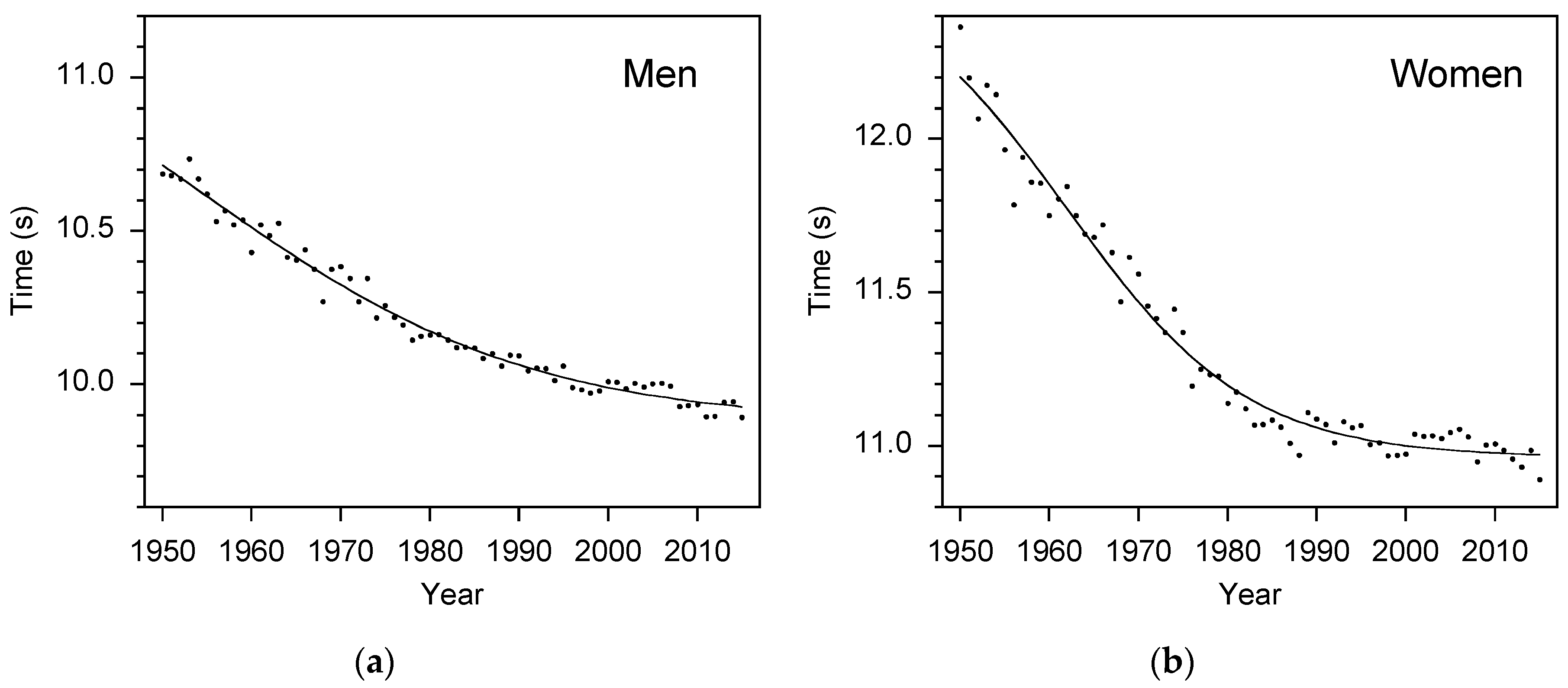
2. Methods
2.1. Corrections for Wind and Historical Trend
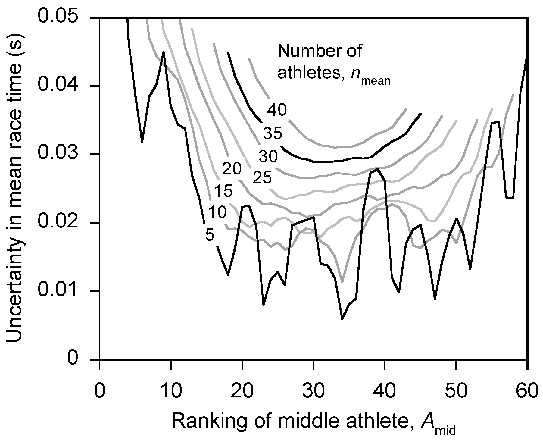
2.2. Calculation of Mean Race Time for an Olympic Games Competition
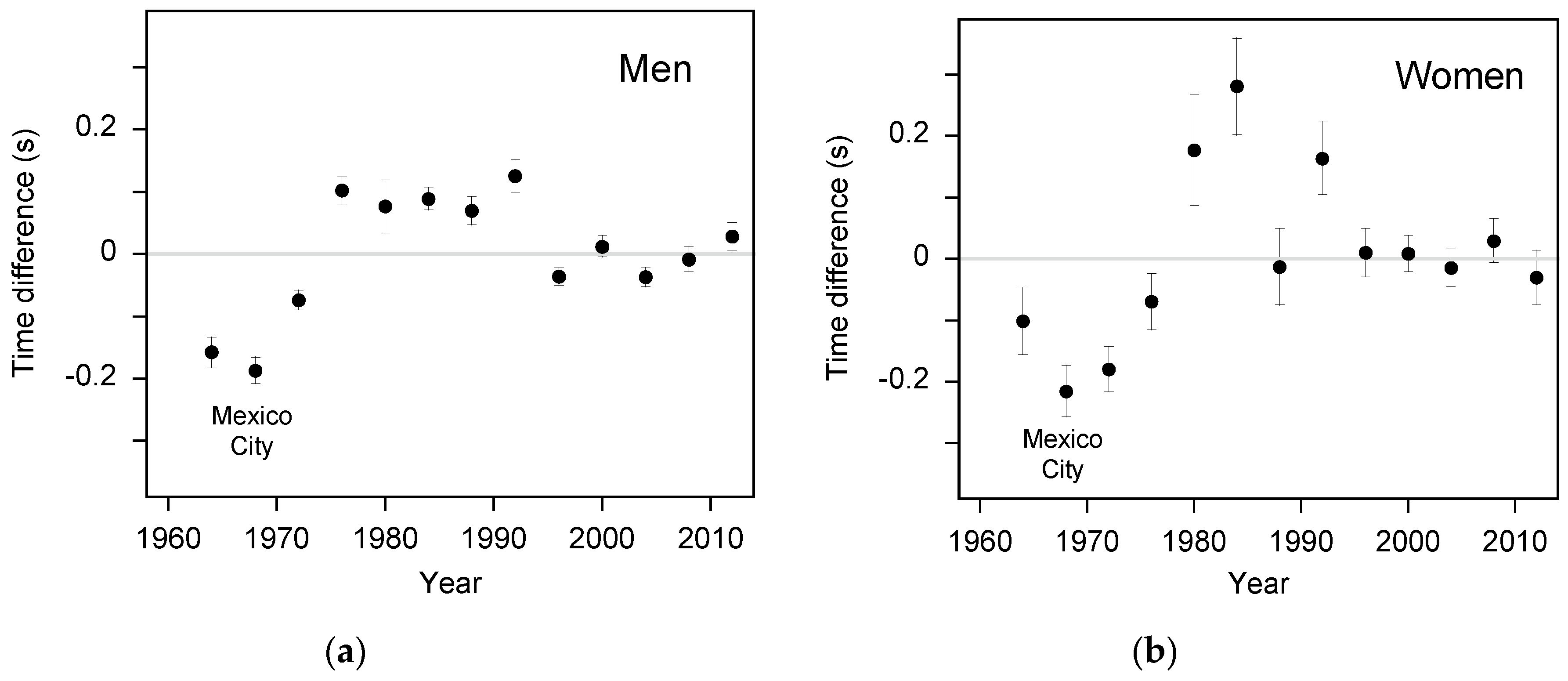
2.3. Time Advantage of Mexico City
2.4. Other Confounding Factors
3. Results
4. Discussion
4.1. Other Competition Analyses and Mathematical Models
4.2. Implications for IAAF Rules
5. Conclusions
Conflicts of Interest
References
- International Association of Athletic Federations (IAAF). IAAF Competition Rules 2016–2017; International Association of Athletic Federations: Monaco, Monaco, 2015; pp. 168–169; 269–279. [Google Scholar]
- Hollings, S.C.; Hopkins, W.G.; Hume, P.A. Environmental and venue-related factors affecting the performance of elite male track athletes. Eur. J. Sport Sci. 2012, 12, 201–206. [Google Scholar] [CrossRef]
- Hymans, R. The Need for Altitude and Non-Altitude World Records. In Athletics 1990: The International Track and Field Annual; Matthews, P., Ed.; Sports World: London, UK, 1990; pp. 145–149. [Google Scholar]
- Jokl, E.; Jokl, P. Analysis of winning times of track races for men in Mexico City in 1968 and Munich in 1972. Olympic Rev. 1972, 60–61, 461–464. [Google Scholar]
- Matthews, P. (Ed.) Athletics 2015: The International Track and Field Annual; SportsBooks: York, UK, 2015; pp. 255–256.
- Ward-Smith, A.J. Air resistance and its influence on the biomechanics and energetics of sprinting at sea level and at altitude. J. Biomech. 1984, 17, 339–347. [Google Scholar] [CrossRef]
- Péronnet, F.; Thibault, G.; Cousineau, D.L. A theoretical analysis of the effect of altitude on running performance. J. Appl. Physiol. 1991, 70, 399–404. [Google Scholar]
- Arsac, L.M. Effects of altitude on the energetics of human best performances in 100 m running: A theoretical analysis. Eur. J. Appl. Physiol. 2002, 87, 78–84. [Google Scholar] [CrossRef] [PubMed]
- Behncke, H. Optimization models for the force and energy in competitive running. J. Math. Biol. 1997, 35, 375–390. [Google Scholar] [CrossRef] [PubMed]
- Dapena, J.; Feltner, M.E. Effects of wind and altitude on the times of 100-meter sprint races. Int. J. Sport Biomech. 1987, 3, 6–39. [Google Scholar] [CrossRef]
- Mureika, J.R. A quasi-physical model of the 100 m dash. Can. J. Phys. 2001, 79, 697–713. [Google Scholar] [CrossRef]
- Jánosi, I.M.; Bántay, P. Statistical test of throwing events on the rotating earth: Lack of correlations between range and geographic location. Eur. Phys. J. B 2002, 30, 411–415. [Google Scholar] [CrossRef]
- Lindsey, B.I. Sports records as biological data. J. Biol. Educ. 1975, 9, 89–91. [Google Scholar] [CrossRef]
- Linthorne, N.P. The effect of wind on 100-m sprint times. J. Appl. Biomech. 1994, 10, 110–131. [Google Scholar]
- International Association of Athletic Federations (IAAF). IAAF Scoring Tables for Combined Events; International Association of Athletic Federations: Monaco, Monaco, 2001; p. 25. [Google Scholar]
- Cleveland, W.S. The Elements of Graphing Data; Hobart Press: Summit, NJ, USA, 1994; pp. 126–132; 168–180. [Google Scholar]
- Motulsky, H.; Christopoulos, A. Fitting Models to Biological Data Using Linear and Nonlinear Regression; Oxford University Press: Oxford, UK, 2004; pp. 147–148. [Google Scholar]
- Taylor, J.R. An Introduction to Error Analysis: The Study of Uncertainties in Physical Measurement, 2nd ed.; University Science Books: Sausalito, CA, USA, 1997; p. 110. [Google Scholar]
- Richards, F.J. A flexible growth function for empirical use. J. Exp. Bot. 1959, 10, 290–300. [Google Scholar] [CrossRef]
- Mureika, J.R. The effects of temperature, humidity, and barometric pressure on short-sprint race times. Can. J. Phys. 2006, 84, 311–324. [Google Scholar] [CrossRef]
- Ward-Smith, A.J. New insights into the effect of wind assistance on sprinting performance. J. Sports Sci. 1999, 17, 325–334. [Google Scholar] [CrossRef] [PubMed]
- Stacey, F.D.; Davis, P.M. Physics of the Earth, 4th ed.; Cambridge University Press: Cambridge, UK, 2008; p. 123. [Google Scholar]


© 2016 by the author; licensee MDPI, Basel, Switzerland. This article is an open access article distributed under the terms and conditions of the Creative Commons Attribution (CC-BY) license (http://creativecommons.org/licenses/by/4.0/).
Share and Cite
Linthorne, N.P. Improvement in 100-m Sprint Performance at an Altitude of 2250 m. Sports 2016, 4, 29. https://doi.org/10.3390/sports4020029
Linthorne NP. Improvement in 100-m Sprint Performance at an Altitude of 2250 m. Sports. 2016; 4(2):29. https://doi.org/10.3390/sports4020029
Chicago/Turabian StyleLinthorne, Nicholas P. 2016. "Improvement in 100-m Sprint Performance at an Altitude of 2250 m" Sports 4, no. 2: 29. https://doi.org/10.3390/sports4020029
APA StyleLinthorne, N. P. (2016). Improvement in 100-m Sprint Performance at an Altitude of 2250 m. Sports, 4(2), 29. https://doi.org/10.3390/sports4020029