Taxonomic and Functional Ant Diversity Along tropical, Subtropical, and Subalpine Elevational Transects in Southwest China

 , ,
, ,
Abstract
:1. Introduction
2. Materials and Methods
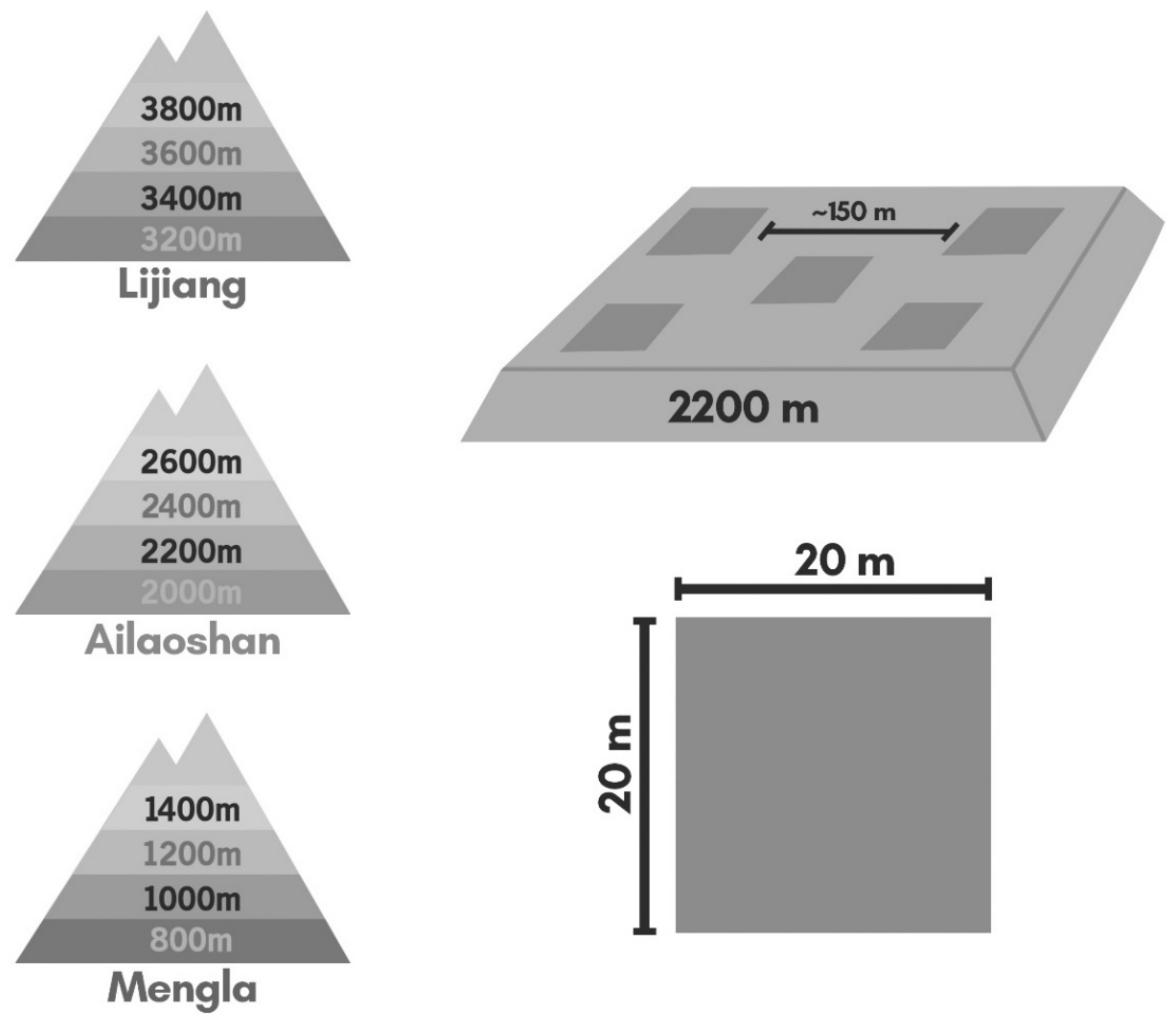
2.1. Study Site
2.2. Field Sampling
- Litter extraction—Two sets of 1 m2 of leaf litter were collected at each plot. Leaf litter samples were taken just outside and on opposite sides of the plot to minimize disturbances within the plot, and to increase spatial coverage. Each 1 m2 sample was taken from four 0.25 m2 quadrats (50 cm × 50 cm) at least 5 m away from each other. Care was taken not to collect thick rain-washed deposits of litter and soil. From each quadrat, all litter and loose surface soil were collected by hand, sieved with a litter sifter, and processed using a Tullgren funnel for 24 to 36 hours, depending on the litter’s water content. Two sets of samples from each plot were pooled before analysis.
- Bark spray—We selected two sets of five trees greater than 30 cm dbh located outside and on opposite sides of the plot. We specifically targeted trees encrusted with vines, epiphytes, or moss to increase the number of ant species and individuals. We placed a rectangular sheet of nylon at the base of each tree and sprayed pyrethroid insecticide from the base to approximately 3 m up the trunk. Catches fallen into the nylon sheets were collected at least 15 minutes after spraying. As with the litter extraction method, two sets of samples from each plot were pooled before data analysis.
- Malaise trap—A Townes Malaise trap was set just outside each plot and operated for 10 days. Although this trapping method targets flying insects such as flies and wasps, wingless, primarily arboreal, ants were often collected.
- Pitfall traps—A total of 10 × 120 mL pitfall traps, each with an internal diameter of 44 mm and filled with 95% ethanol, were placed in each plot and left open for ten days. The 10 traps were installed along a diagonal line of the plot, approximately 2.5 m away from each other. A black plastic plate of 15 cm × 15 cm was suspended 4–5 cm above the pitfall traps to intercept rainfall. Samples from each plot were also pooled before data analysis.
- Hand collection—At each plot, hand collections were performed once within the 50 m radius of the plot for one hour during the day (09:00–17:00 h). Foraging ants and ants in nests were searched and collected by hand from the ground, foliage, and logs by CJB.

| Trait | Justification | References |
|---|---|---|
| Weber’s length (WL) | Commonly used as a proxy for ant body size, which reflects the amount and type of resource exploited. May also reflect ability to nest in vegetation. | [15,28,29] |
| Relative eye length (RelEL) | While eyes are used by ants for navigation and recognition of predator and prey, eye size may also be indicative of when (i.e., diurnal or nocturnal) and where ants forage, as well as their dietary preference (predators tend to have smaller eyes than omnivores). | [29,30,31] |
| Relative scape length (RelSL) | May determine ants’ effective range of sensitivity to chemosensory signals | [31] |
| Relative mandible length (RelML) | Indicator of diet type, with predatory ants having longer mandibles | [31,32] |
| Relative hindleg length (RelHL) | Related to locomotion speed as well as ants’ capacity to navigate through crevices of varying sizes and the amount of load they can carry. May also indicate the type of diet, as ants with shorter RelHL tend to be predators. | [31,33,34] |
2.3. Functional Traits
2.4. Data Analysis
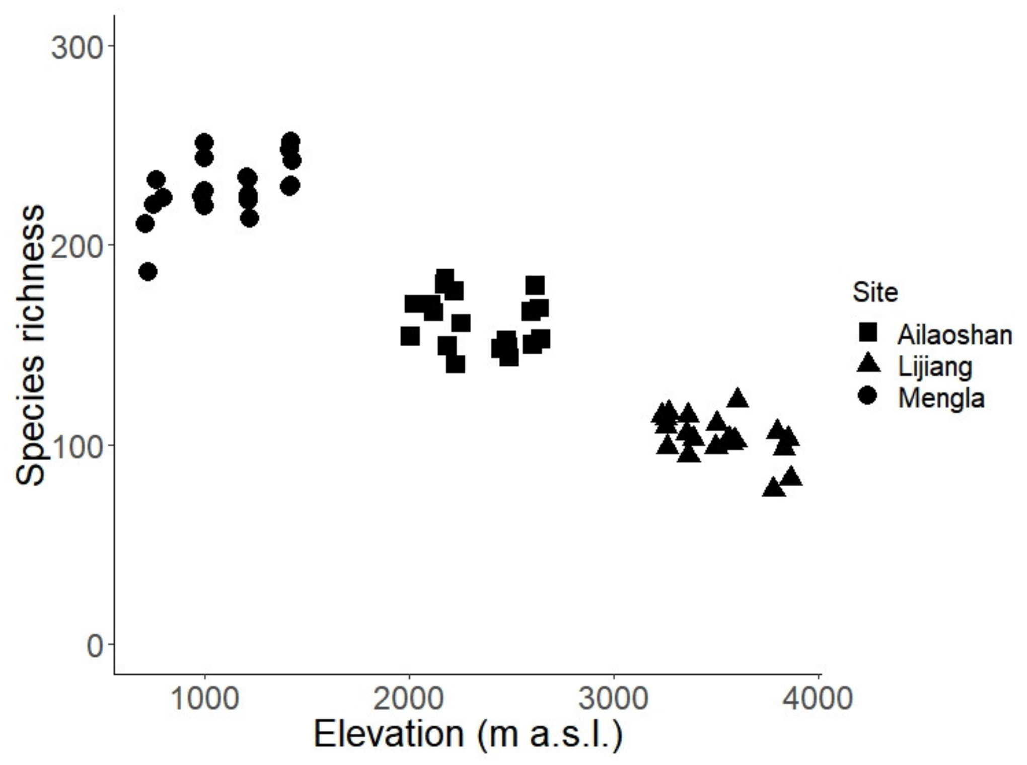
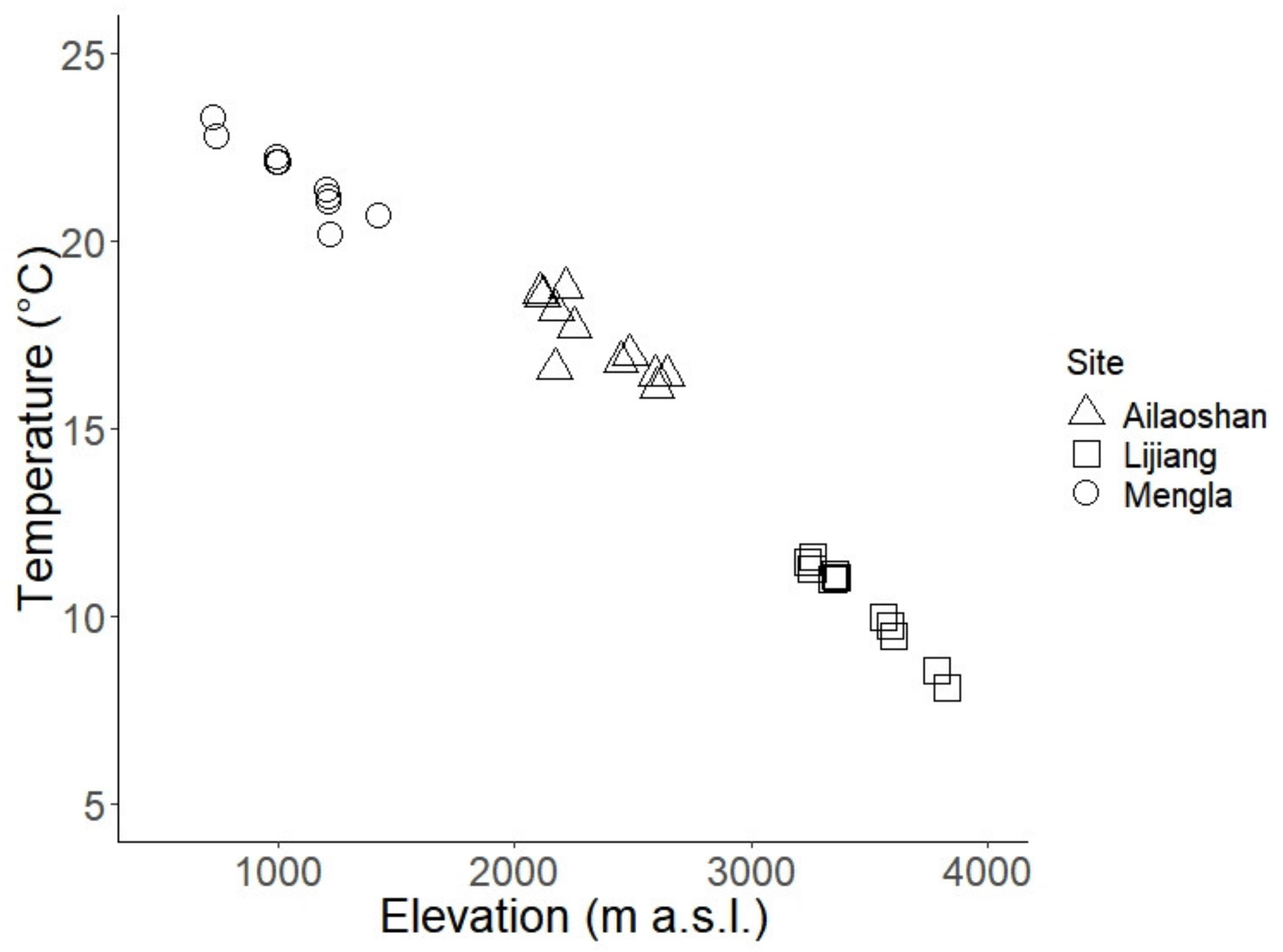
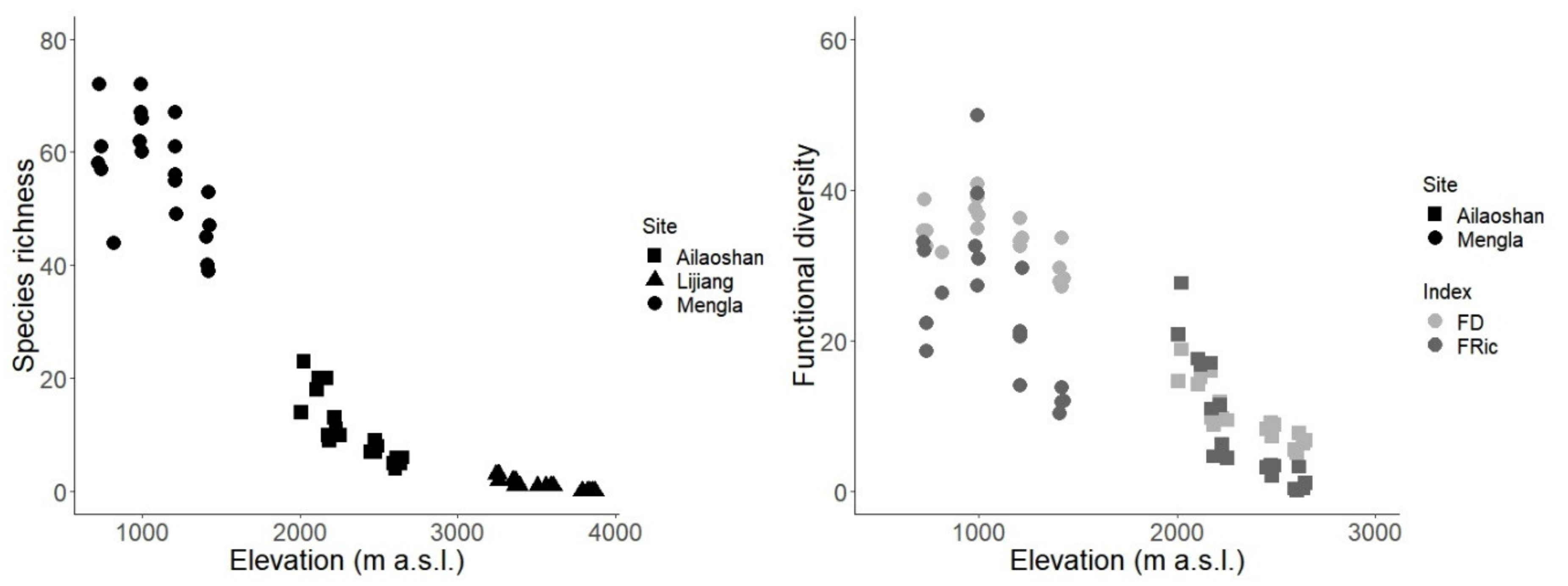
3. Results
4. Discussion
5. Conclusions
Supplementary Materials
Author Contributions
Funding
Acknowledgments
Conflicts of Interest
Appendix A
References
- Linnaeus, C. On the growth of the habitable earth. In Select dissertations from the Amoenitates Academicae; Robinson, G., Robson, J., Eds.; FJ Brand, Trans: London, UK, 1781; Volume 1, pp. 71–127. [Google Scholar]
- Willdenow, K.L. The Principles of Botany, and Vegetable Physiology; Blackwood, Cadell and Davies: London, UK, 1805. [Google Scholar]
- Von Humboldt, A.; Bonpland, A. Essay on the geography of plants with a physical tableau of the equinoctial regions (S Romanowski, Trans.). In Essay on the Geography of Plants; Jackson, S.T., Ed.; University of Chicago Press: Chicago, IL, USA, 1807; pp. 57–143. [Google Scholar]
- Hillebrand, H. On the generality of the latitudinal diversity gradient. Am. Nat. 2004, 163, 192–211. [Google Scholar] [CrossRef]
- Guo, Q.; Kelt, D.A.; Sun, Z.; Liu, H.; Hu, L.; Ren, H.; Wen, J. Global variation in elevational diversity patterns. Sci. Rep. 2013, 3, 3007. [Google Scholar] [CrossRef] [PubMed]
- Beck, J.; McCain, C.M.; Axmacher, J.C.; Ashton, L.A.; Bärtschi, F.; Brehm, G.; Choi, S.W.; Cizek, O.; Colwell, R.K.; Fiedler, K.; et al. Elevational species richness gradients in a hyperdiverse insect taxon: A global meta-study on geometrid moths. Global Ecol. Biogeogr. 2017, 26, 412–424. [Google Scholar] [CrossRef]
- Quintero, I.; Jetz, W. Global elevational diversity and diversification of birds. Nature 2018, 555, 246–250. [Google Scholar] [CrossRef]
- Brown, J.H. Why are there so many species in the tropics? J. Biogeogr. 2014, 41, 8–22. [Google Scholar] [CrossRef] [PubMed]
- Sanders, N.J.; Rahbek, C. The patterns and causes of elevational diversity gradients. Ecography 2012, 35, 1–3. [Google Scholar] [CrossRef]
- Laiolo, P.; Pato, J.; Obeso, J.R. Ecological and evolutionary drivers of the elevational gradient of diversity. Ecol. Lett. 2018, 21, 1022–1032. [Google Scholar] [CrossRef] [PubMed]
- Antonelli, A.; Kissling, W.D.; Flantua, S.G.A.; Bermúdez, M.A.; Mulch, A.; Muellner-Riehl, A.N.; Kreft, H.; Linder, H.P.; Badgley, C.; Fjeldså, J.; et al. Geological and climatic influences on mountain biodiversity. Nat. Geosci. 2018, 11, 718–725. [Google Scholar] [CrossRef]
- Weiher, E. A primer of trait and functional diversity. In Biological Diversity: Frontiers in Measurement and Assessment; Magurran, A.E., McGill, M.J., Eds.; Oxford University Press: New York, NY, USA, 2011; pp. 175–193. [Google Scholar]
- Weiher, E.; Keddy, P.A. Assembly rules, null models, and trait dispersion: new questions from old patterns. Oikos 1995, 74, 159–164. [Google Scholar] [CrossRef]
- Villéger, S.; Grenouillet, G.; Brosse, S. Decomposing β-diversity reveals that low functional β-diversity is driven by low functional turnover in European fish assemblages. Global Ecol. Biogeogr. 2013, 22, 671–681. [Google Scholar] [CrossRef]
- Bishop, T.R.; Robertson, M.P.; van Rensburg, B.J.; Parr, C.L. Contrasting species and functional beta diversity in montane ant assemblages. J. Biogeogr. 2015, 42, 1776–1786. [Google Scholar] [CrossRef]
- Kaltsas, D.; Dede, K.; Giannaka, J.; Nasopoulou, T.; Kechagioglou, S.; Grigoriadou, E.; Raptis, D.; Damos, P.; Vasiliadis, I.; Christopoulos, V.; et al. Taxonomic and functional diversity of butterflies along an altitudinal gradient in two NATURA 2000 sites in Greece. Insect Conserv. Diversity 2018, 11, 464–478. [Google Scholar] [CrossRef]
- Nunes, C.A.; Quintino, A.V.; Constantino, R.; Negreiros, D.; Júnior, R.R.; Fernandes, G.W. Patterns of taxonomic and functional diversity of termites along a tropical elevational gradient. Biotropica 2017, 49, 186–194. [Google Scholar] [CrossRef]
- Hölldobler, B.; Wilson, E.O. The Ants; Harvard University Press: Cambridge, MA, USA, 1990. [Google Scholar]
- Economo, E.P.; Narula, N.; Friedman, N.R.; Weiser, M.D.; Guénard, B. Macroecology and macroevolution of the latitudinal diversity gradient in ants. Nat. Commun. 2018, 9, 1778. [Google Scholar] [CrossRef] [PubMed]
- Dunn, R.R.; Agosti, D.; Andersen, A.N.; Arnan, X.; Bruhl, C.A.; Cerdá, X.; Ellison, A.M.; Fisher, B.L.; Fitzpatrick, M.C.; Gibb, H.; et al. Climatic drivers of hemispheric asymmetry in global patterns of ant species richness. Ecol. Lett. 2009, 12, 324–333. [Google Scholar] [CrossRef] [PubMed]
- Vasconcelos, H.L.; Maravalhas, J.B.; Feitosa, R.M.; Pacheco, R.; Neves, K.C.; Andersen, A.N. Neotropical savanna ants show a reversed latitudinal gradient of species richness, with climatic drivers reflecting the forest origin of the fauna. J. Biogeogr. 2018, 45, 248–258. [Google Scholar] [CrossRef]
- Szewczyk, T.; McCain, C.M. A systematic review of global drivers of ant elevational diversity. PLoS ONE 2016, 11, e0155404. [Google Scholar] [CrossRef] [PubMed]
- Reymond, A.; Purcell, J.; Cherix, D.; Guisan, A.; Pellissier, L. Functional diversity decreases with temperature in high elevation ant fauna. Ecol. Entomol. 2013, 38, 364–373. [Google Scholar] [CrossRef]
- Ashton, L.A.; Nakamura, A.; Burwell, C.J.; Tang, Y.; Cao, M.; Whitaker, T.; Sun, Z.; Huang, H.; Kitching, R.L. Elevational sensitivity in an Asian ‘hotspot’: Oth diversity across elevational gradients in tropical, sub-tropical and sub-alpine China. Sci. Rep. 2016, 6, 26513. [Google Scholar] [CrossRef]
- Yang, Y.; Tian, K.; Hao, J.; Pei, S.; Yang, Y. Biodiversity and biodiversity conservation in Yunnan, China. Biodivers. Conserv. 2004, 13, 813–826. [Google Scholar] [CrossRef]
- Myers, N.; Mittermeier, R.A.; Mittermeier, C.G.; da Fonseca, G.A.B.; Kent, J. Biodiversity hotspots for conservation priorities. Nature 2000, 403, 853–858. [Google Scholar] [CrossRef] [PubMed]
- Burwell, C.J.; Nakamura, A. Can changes in ant diversity along elevational gradients in tropical and subtropical Australian rainforests be used to detect a signal of past lowland biotic attrition? Austral Ecol. 2016, 41, 209–218. [Google Scholar] [CrossRef]
- Arnan, X.; Cerdá, X.; Rodrigo, A.; Retana, J. Response of ant functional composition to fire. Ecography 2013, 36, 1182–1193. [Google Scholar] [CrossRef]
- Moretti, M.; Dias, A.T.; De Bello, F.; Altermatt, F.; Chown, S.L.; Azcárate, F.M.; Bell, J.R.; Fournier, B.; Hedde, M.; Hortal, J.; et al. Handbook of protocols for standardized measurement of terrestrial invertebrate functional traits. Funct. Ecol. 2017, 31, 558–567. [Google Scholar] [CrossRef]
- Bihn, J.H.; Gebauer, G.; Brandl, R. Loss of functional diversity of ant assemblages in secondary tropical forests. Ecology 2010, 91, 782–792. [Google Scholar] [CrossRef] [PubMed]
- Weiser, M.D.; Kaspari, M. Ecological morphospace of New World ants. Ecol. Entomol. 2006, 31, 131–142. [Google Scholar] [CrossRef]
- Silva, R.R.; Brandão, R.F. Morphological patterns and ant community organization in leaf-litter ant assemblages. Ecol. Monogr. 2010, 80, 107–124. [Google Scholar] [CrossRef]
- Feener, D.H., Jr.; Lighton, J.R.B.; Bartholomew, G.A. Curvilinear allometry, energetics and foraging ecology: A comparison of leaf-cutting ants and army ants. Funct. Ecol. 1988, 2, 509–520. [Google Scholar] [CrossRef]
- Kaspari, M.; Weiser, M.D. The size-grain hypothesis and interspecific scaling in ants. Funct. Ecol. 1999, 13, 530–538. [Google Scholar] [CrossRef]
- Liu, C.; Guénard, B.; Blanchard, B.; Peng, Y.Q.; Economo, E.P. Reorganization of taxonomic, functional, and phylogenetic ant biodiversity after conversion to rubber plantation. Ecol. Monogr. 2016, 86, 215–227. [Google Scholar] [CrossRef]
- Petchey, O.L.; Gaston, K.J. Functional diversity (FD), species richness and community composition. Ecol. Lett. 2002, 5, 402–411. [Google Scholar] [CrossRef]
- Villéger, S.; Mason, N.W.H.; Mouillot, D. New multidimensional functional diversity indices for a multifaceted framework in functional ecology. Ecology 2008, 89, 2290–2301. [Google Scholar] [CrossRef]
- Cornwell, W.K.; Schwilk, D.W.; Ackerly, D.D. A trait-based test for habitat filtering: Convex hull volume. Ecology 2006, 87, 1465–1471. [Google Scholar] [CrossRef]
- Mouchet, M.A.; Villéger, S.; Mason, N.W.H.; Mouillot, D. Functional diversity measures: An overview of their redundancy and their ability to discriminate community assembly rules. Funct. Ecol. 2010, 24, 867–876. [Google Scholar] [CrossRef]
- Swenson, N.G. Functional and Phylogenetic Diversity in R; Springer: New York, NY, USA, 2014. [Google Scholar]
- Kembel, S.W.; Cowan, P.D.; Helmus, M.R.; Cornwell, W.K.; Morlon, H.; Ackerly, D.D.; Blomberg, S.P.; Webb, C.O. Picante: R tools for integrating phylogenies and ecology. Bioinformatics 2010, 26, 1463–1464. [Google Scholar] [CrossRef] [PubMed]
- Laliberté, E.; Legendre, P. A distance-based framework for measuring functional diversity from multiple traits. Ecology 2010, 91, 299–305. [Google Scholar] [CrossRef]
- Song, X.; Li, J.; Zhang, W.; Tang, Y.; Sun, Z.; Cao, M. Variant responses of tree seedling to seasonal drought stress along an elevational transect in tropical montane forests. Sci. Rep. 2016, 6, 36438. [Google Scholar] [CrossRef]
- Baselga, A.; Orme, D.O. Betapart: An R package for the study of beta diversity. Methods Ecol. Evol. 2012, 3, 808–812. [Google Scholar] [CrossRef]
- Baselga, A. Partitioning the turnover and nestedness components of beta diversity. Global Ecol. Biogeogr. 2010, 19, 134–143. [Google Scholar] [CrossRef]
- Oksanen, J.; Blanchet, F.G.; Friendly, M.; Kindt, R.; Legendre, P.; McGlinn, D.; Minchin, P.R.; O’Hara, R.B.; Simpson, G.L.; Solymos, P.; et al. Vegan: Community Ecology Package. R package version 2.5-4. 2019. Available online: https://CRAN.R-project.org/package=vegan (accessed on 1 April 2019).
- Gotelli, N.J.; Entsminger, G.L. Swap and fill algorithms in null model analysis: Rethinking the knight’s tour. Oecologia 2001, 129, 281–291. [Google Scholar] [CrossRef] [PubMed]
- McCain, C.M.; Grytnes, J.A. Elevational gradients in species richness. In Encyclopedia of Life Sciences (ELS); John Wiley & Sons, Ltd.: Chichester, UK, 2010. [Google Scholar]
- Wang, R.; Compton, S.G.; Quinnell, R.J.; Peng, Y.Q.; Barwell, L.; Chen, Y. Insect responses to host plant provision beyond natural boundaries: Latitudinal and altitudinal variation in a Chinese fig wasp community. Ecol. Evol. 2015, 5, 3642–3656. [Google Scholar] [CrossRef] [PubMed]
- Parr, C.L.; Dunn, R.R.; Sanders, N.J.; Weiser, M.D.; Photakis, M.; Bishop, T.R.; Fitzpatrick, M.C.; Arnan, X.; Baccaro, F.; Brandão, C.R.; et al. GlobalAnts: A new database on the geography of ant traits (Hymenoptera: Formicidae). Insect Conserv. Divers. 2017, 10, 5–20. [Google Scholar] [CrossRef]
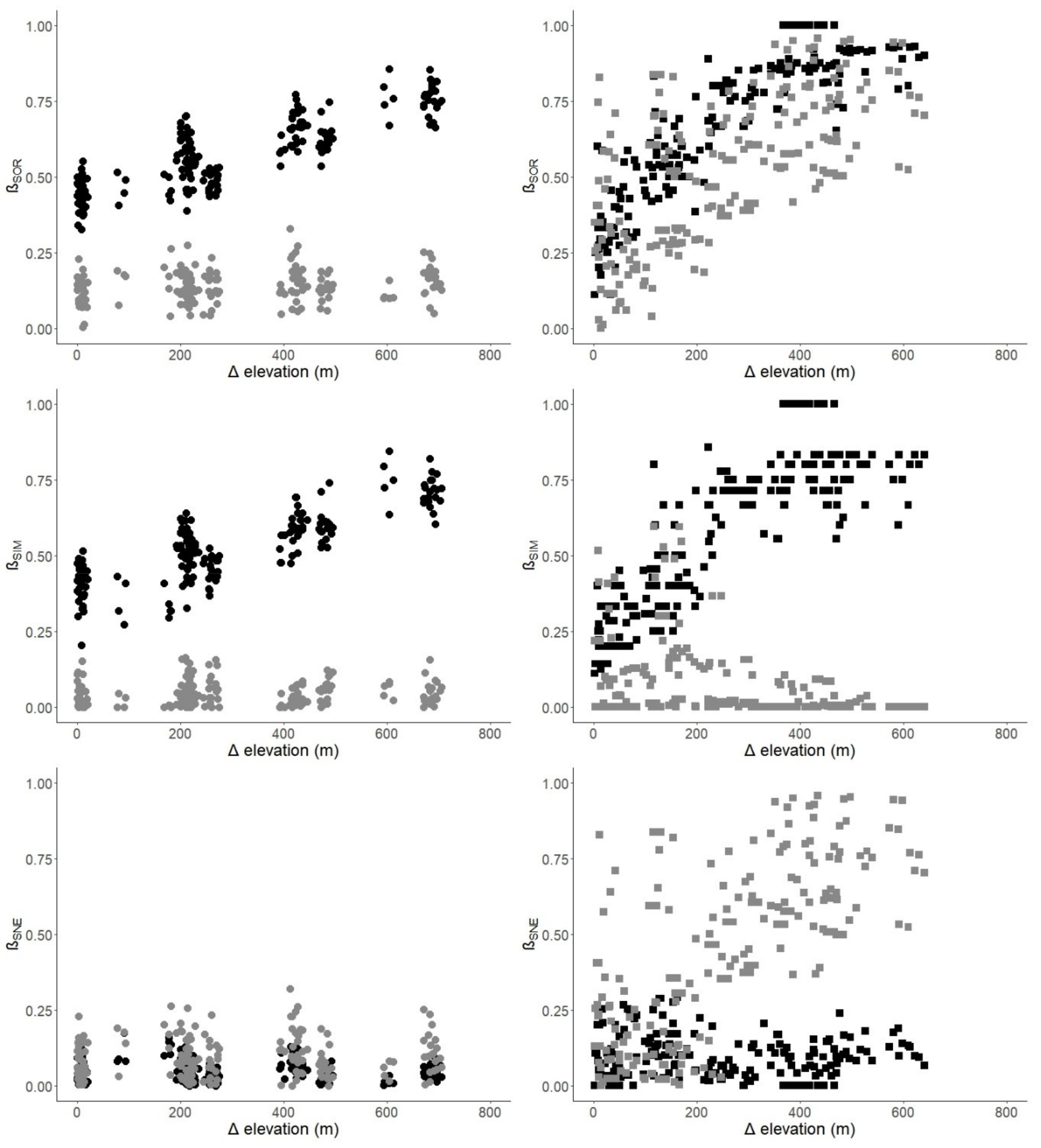
| Index | Mengla | Ailaoshan | ||
|---|---|---|---|---|
| Taxonomic βSOR | 0.826 | (<0.001) | 0.873 | (<0.001) |
| βSIM | 0.813 | (<0.001) | 0.833 | (<0.001) |
| βSNE | −0.044 | (0.690) | −0.088 | (0.893) |
| Functional βSOR | 0.187 | (0.017) | 0.655 | (<0.001) |
| βSIM | 0.096 | (0.123) | −0.347 | (1) |
| βSNE | 0.088 | (0.133) | 0.709 | (<0.001) |
© 2019 by the authors. Licensee MDPI, Basel, Switzerland. This article is an open access article distributed under the terms and conditions of the Creative Commons Attribution (CC BY) license (http://creativecommons.org/licenses/by/4.0/).
Share and Cite
Fontanilla, A.M.; Nakamura, A.; Xu, Z.; Cao, M.; Kitching, R.L.; Tang, Y.; Burwell, C.J. Taxonomic and Functional Ant Diversity Along tropical, Subtropical, and Subalpine Elevational Transects in Southwest China. Insects 2019, 10, 128. https://doi.org/10.3390/insects10050128
Fontanilla AM, Nakamura A, Xu Z, Cao M, Kitching RL, Tang Y, Burwell CJ. Taxonomic and Functional Ant Diversity Along tropical, Subtropical, and Subalpine Elevational Transects in Southwest China. Insects. 2019; 10(5):128. https://doi.org/10.3390/insects10050128
Chicago/Turabian StyleFontanilla, Alyssa M., Akihiro Nakamura, Zhenghui Xu, Min Cao, Roger L. Kitching, Yong Tang, and Chris J. Burwell. 2019. "Taxonomic and Functional Ant Diversity Along tropical, Subtropical, and Subalpine Elevational Transects in Southwest China" Insects 10, no. 5: 128. https://doi.org/10.3390/insects10050128
APA StyleFontanilla, A. M., Nakamura, A., Xu, Z., Cao, M., Kitching, R. L., Tang, Y., & Burwell, C. J. (2019). Taxonomic and Functional Ant Diversity Along tropical, Subtropical, and Subalpine Elevational Transects in Southwest China. Insects, 10(5), 128. https://doi.org/10.3390/insects10050128