Multi-Scenario Species Distribution Modeling


Abstract
:1. Introduction
2. Materials and Methods
2.1. Geographic Extent of Study Area
2.2. Predictor Data
2.3. Dimension Reduction
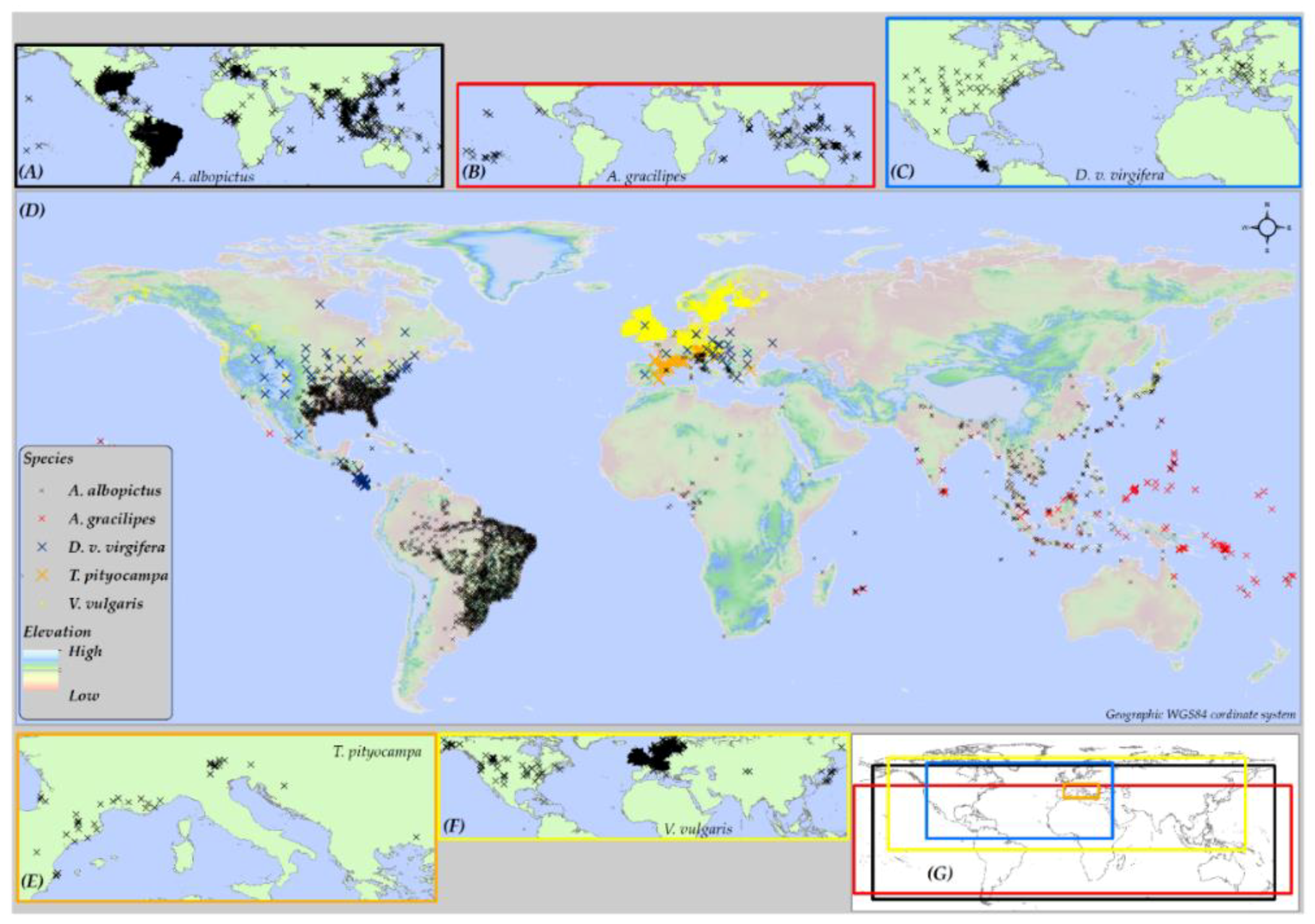
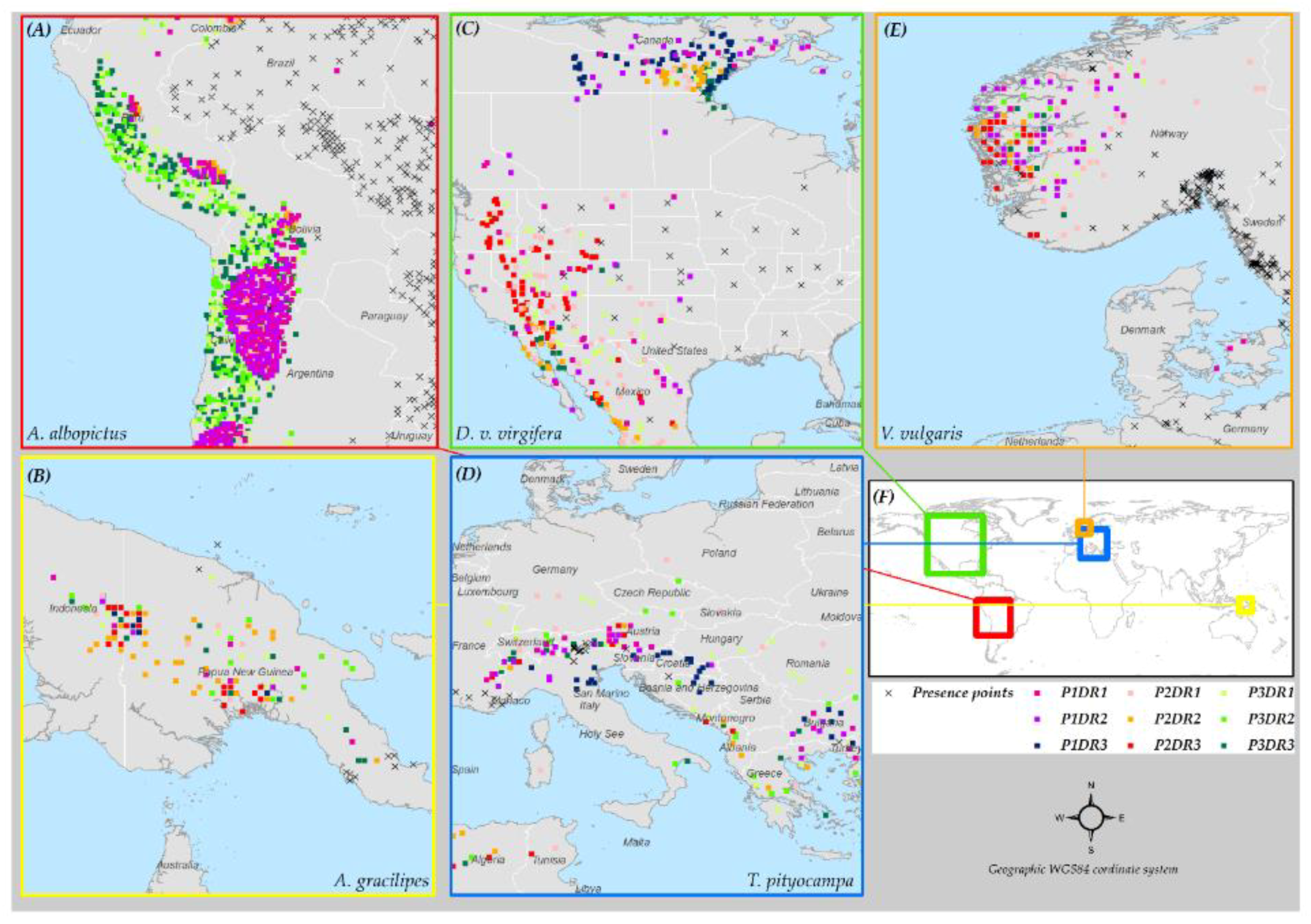
2.4. Species Data
2.5. Model Type
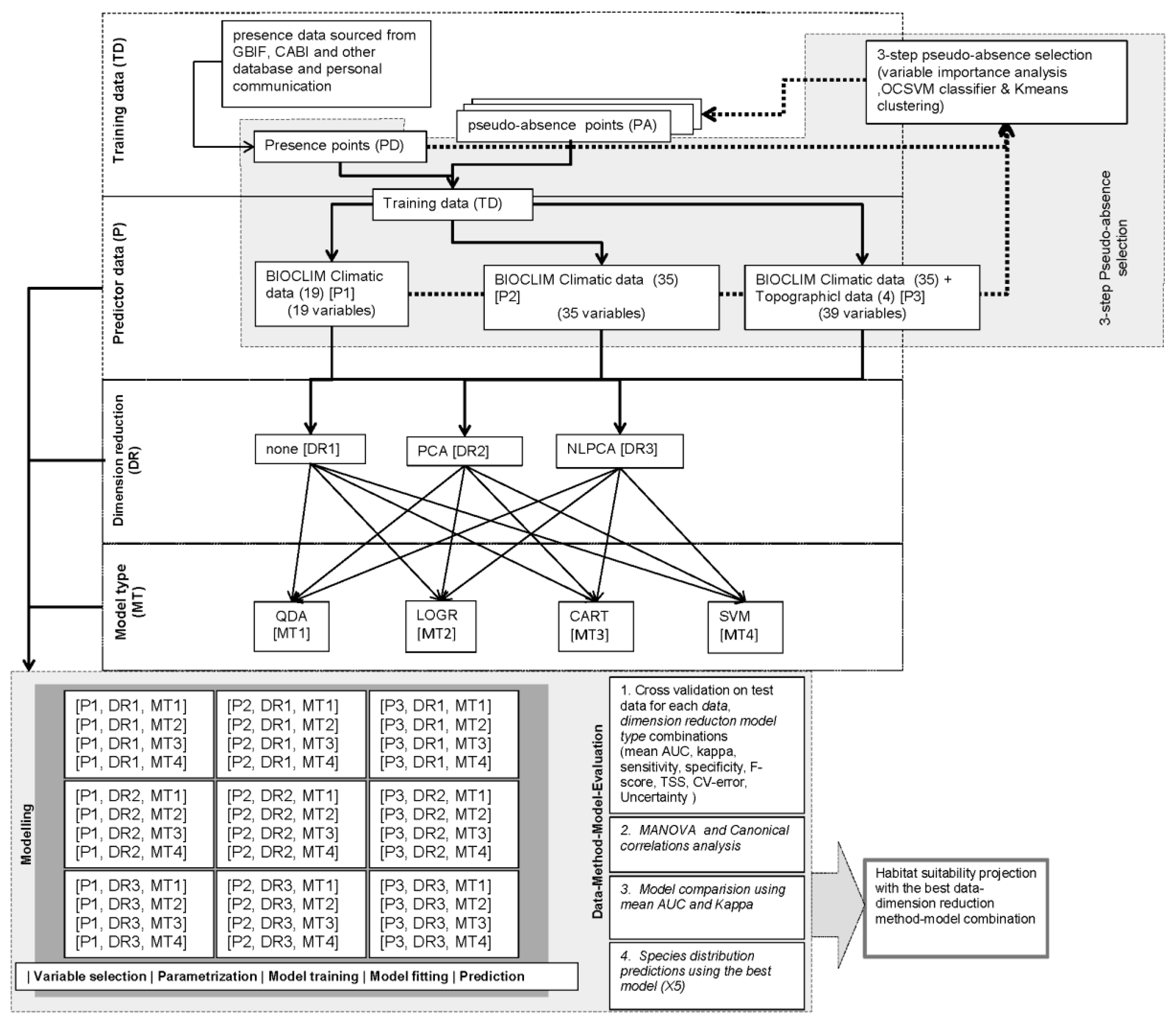
2.6. Research Design and Model Conceptualization
2.7. Model Choice Evaluation
3. Results
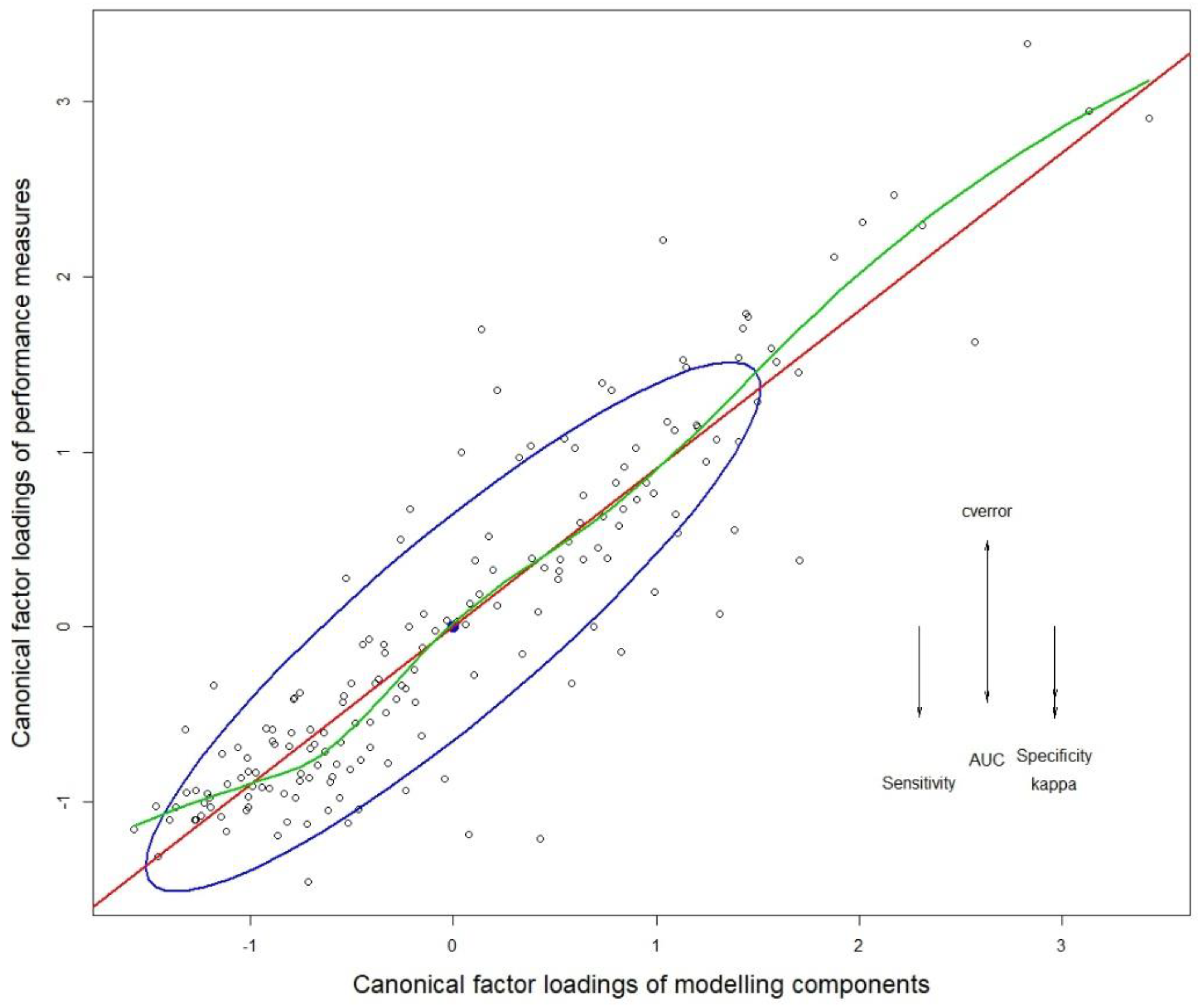
3.1. Multivariate Analysis of Variance (MANOVA)
3.2. Quantifying the Variance Contribution of Modeling Factors
3.3. Species Level Analysis of Variance
3.4. Modeling Components
3.4.1. Species Data
3.4.2. Predictor Choice/Variable Selection
3.4.3. Dimension Reduction
3.4.4. Model Type
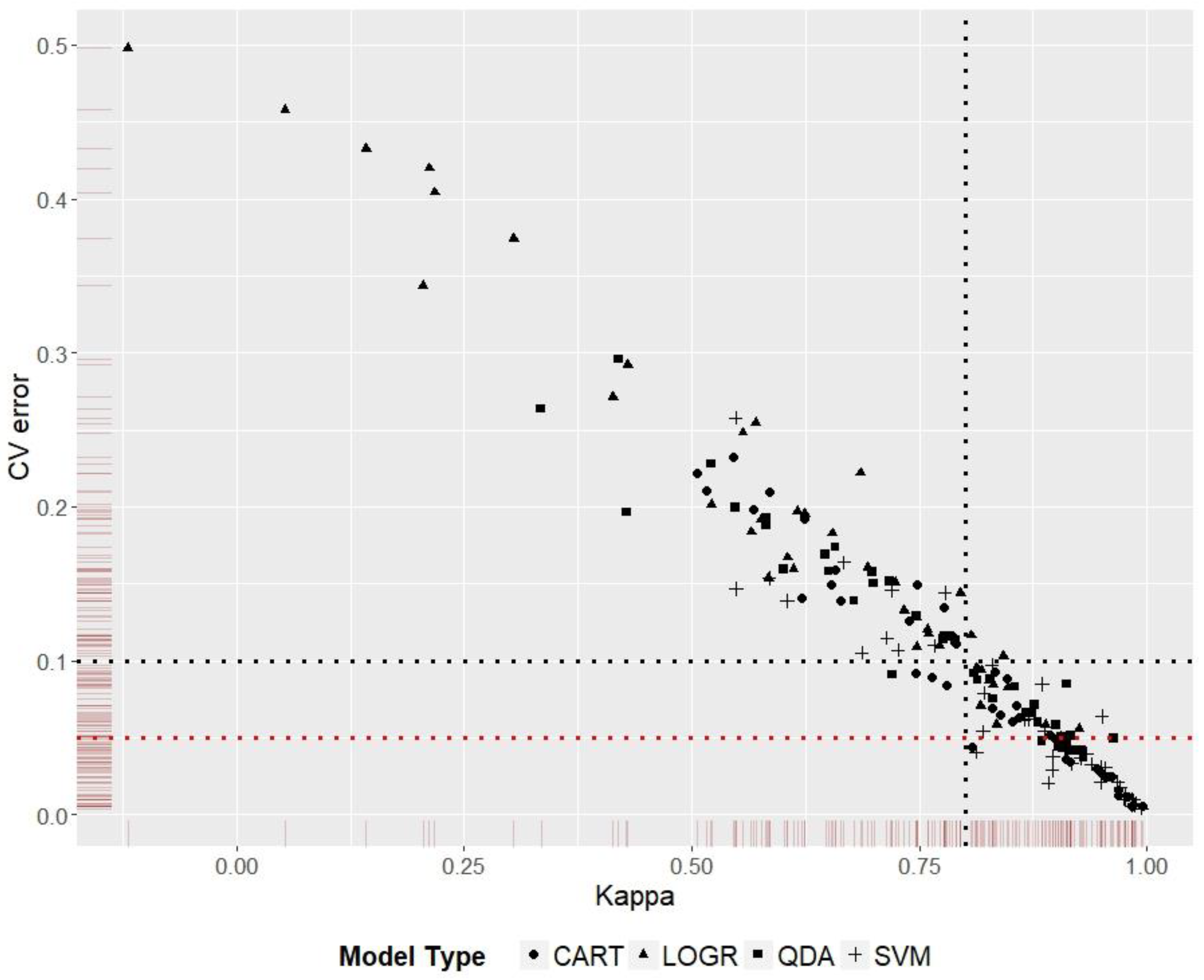
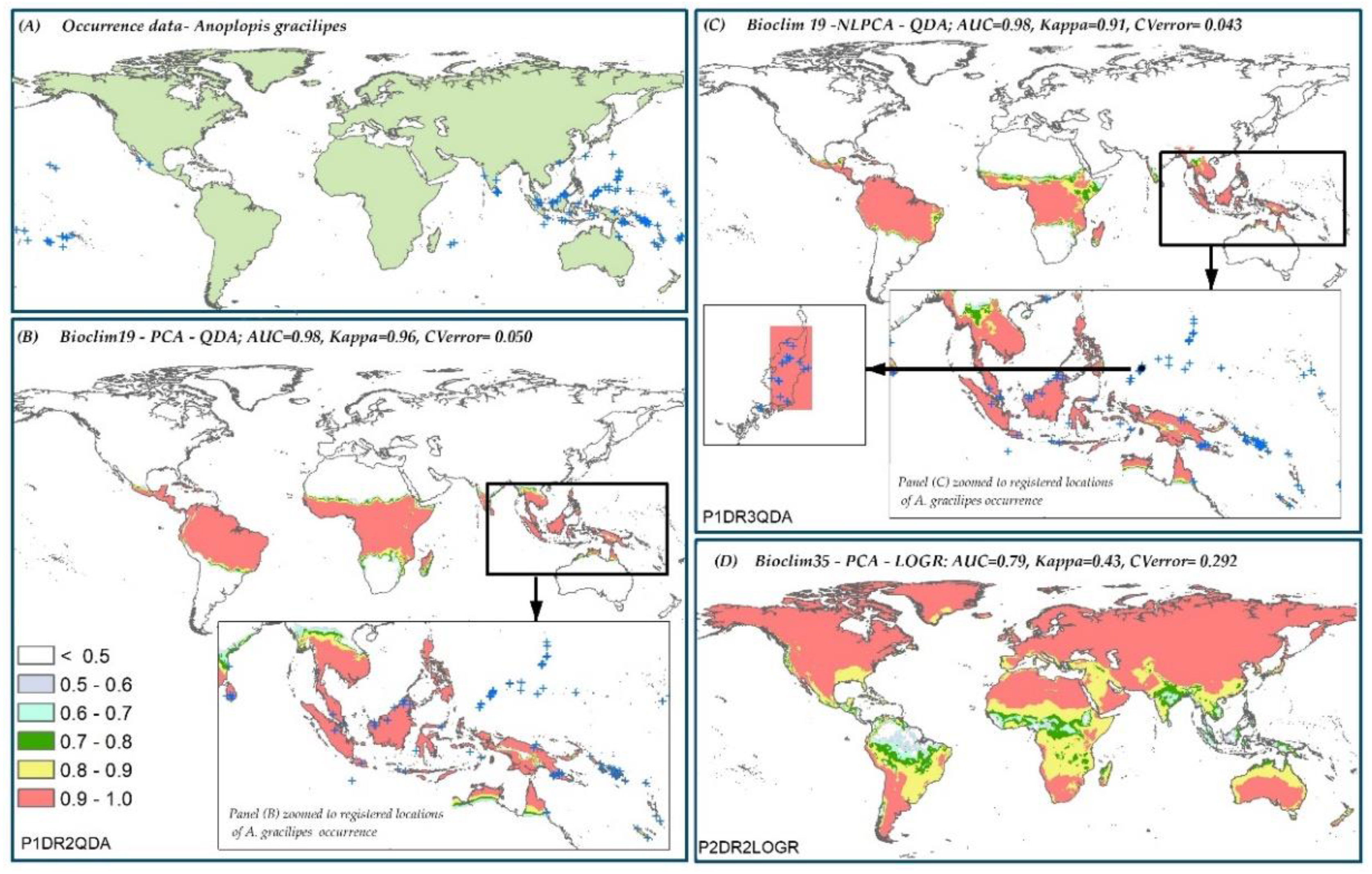
3.5. Model Ranking
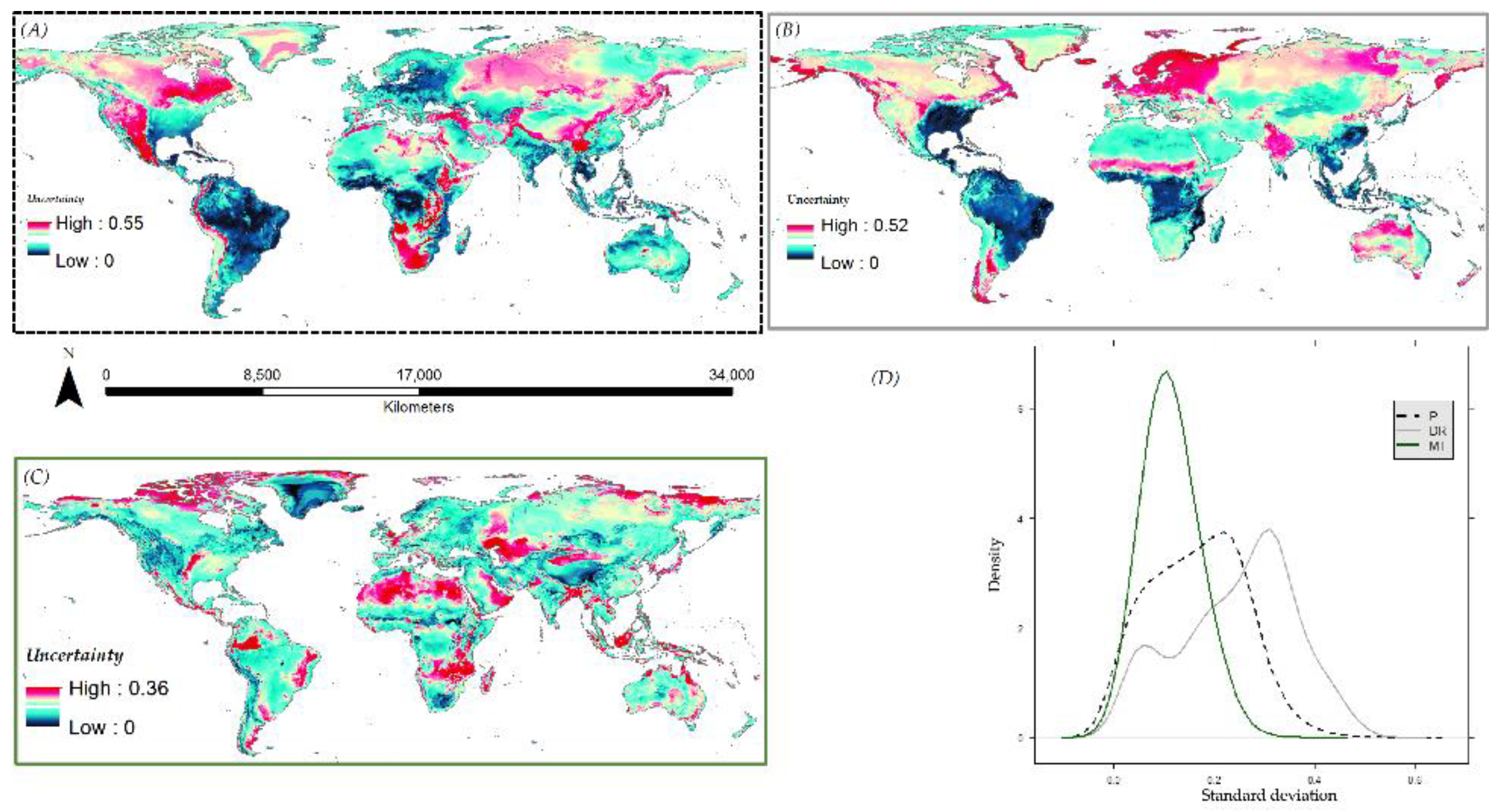
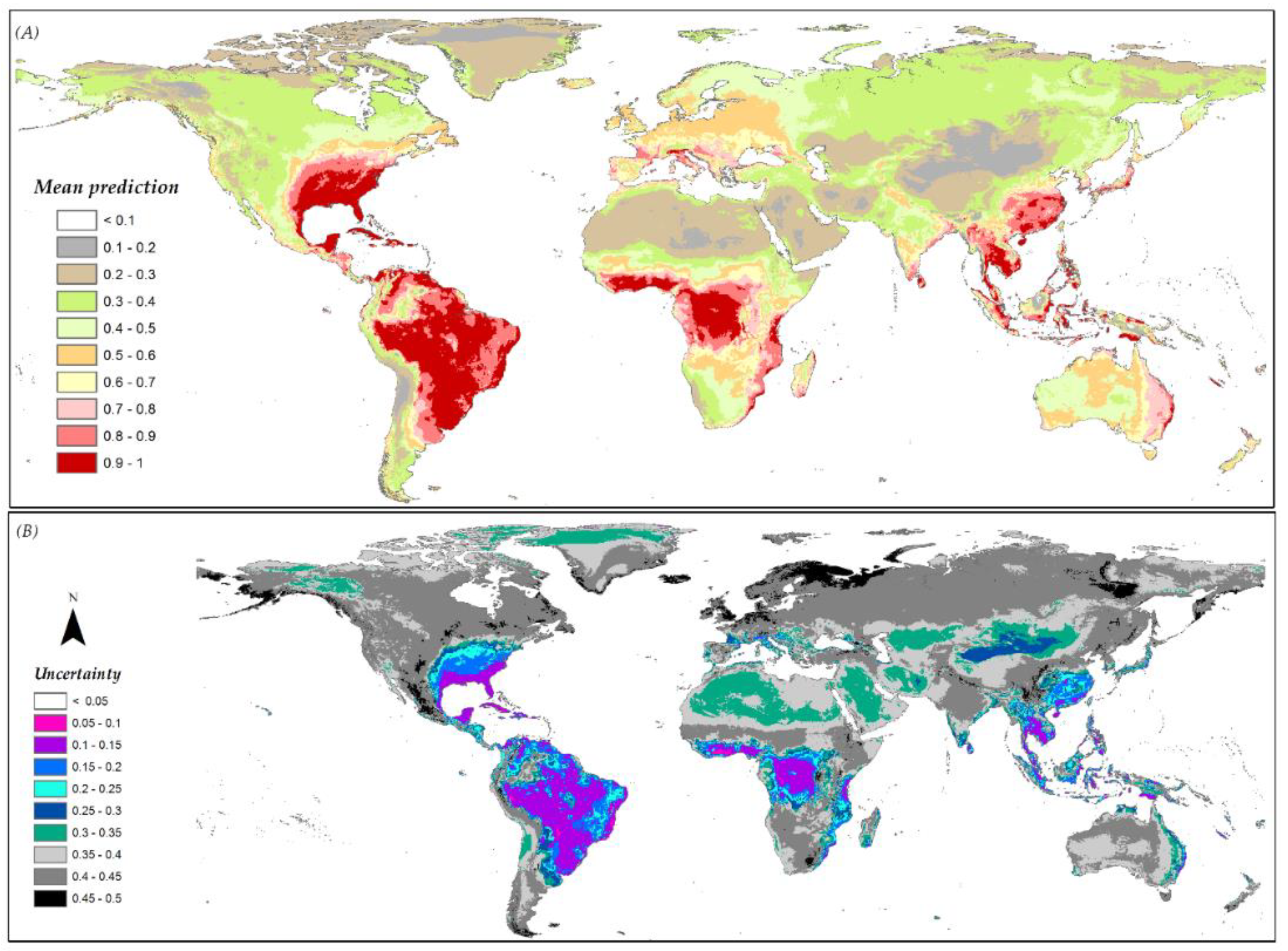
3.6. Species Distribution Predictions and Uncertainty
4. Discussion
5. Conclusions
Supplementary Materials
Author Contributions
Funding
Acknowledgments
Conflicts of Interest
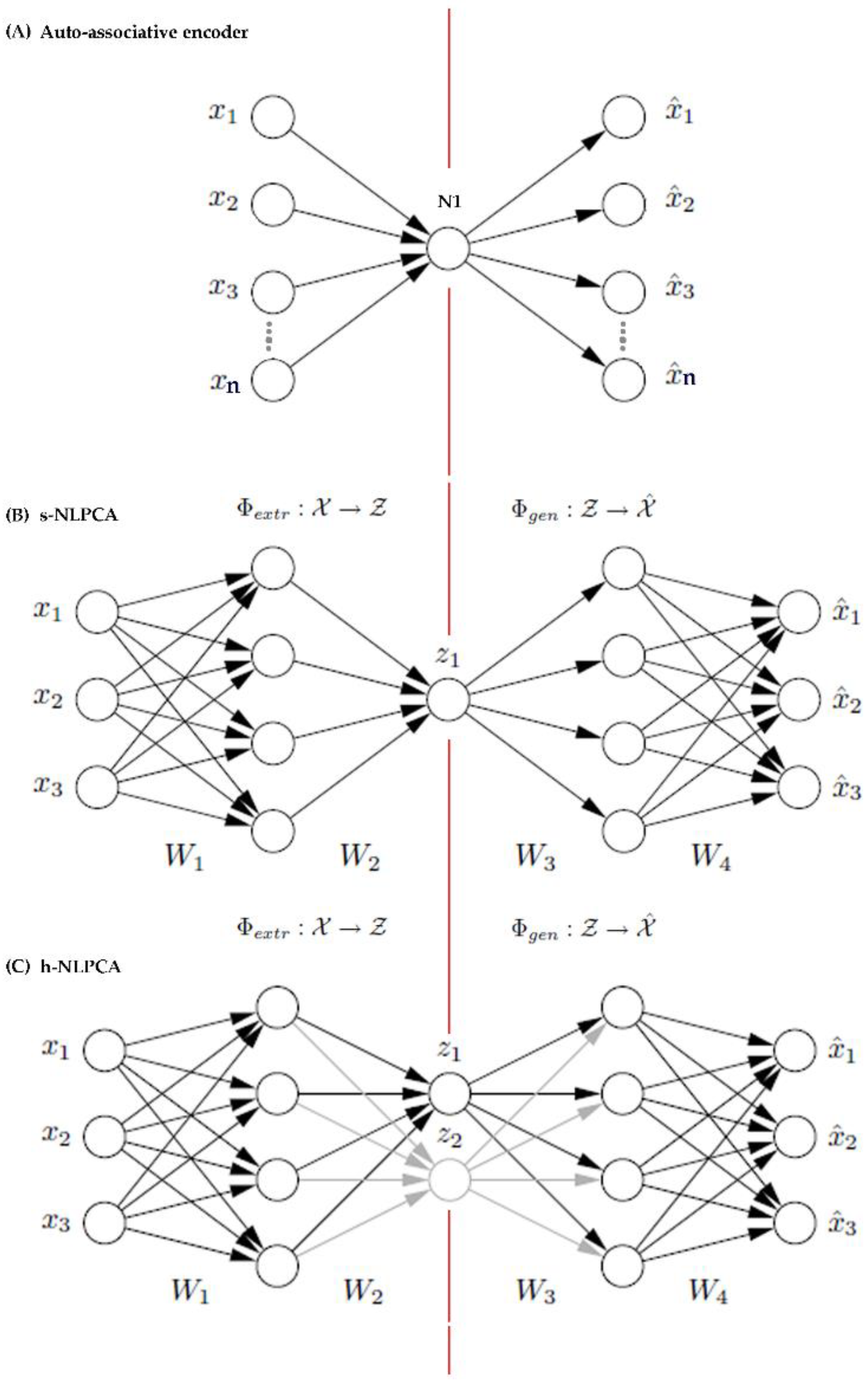
Appendix A. Background on h-NLPCA Dimension Reduction Method

References
- Elith, J.; Leathwick, J.R. Species Distribution Models: Ecological Explanation and Prediction Across Space and Time. Annu. Rev. Ecol. Evol. Syst. 2009, 40, 677–697. [Google Scholar] [CrossRef]
- Elith, J.; Burgman, M.A.; Regan, H.M. Mapping epistemic uncertainties and vague concepts in predictions of species distribution. Ecol. Model. 2002, 157, 313–329. [Google Scholar] [CrossRef]
- Thuiller, W. Patterns and uncertainties of species’ range shifts under climate change. Glob. Change Biol. 2004, 10, 2020–2027. [Google Scholar] [CrossRef]
- Araújo, M.B.; Guisan, A. Five (or so) challenges for species distribution modelling. J. Biogeogr. 2006, 33, 1677–1688. [Google Scholar] [CrossRef]
- Elith, J.; Graham, C.H.; Anderson, R.P.; Dudik, M.; Ferrier, S.; Guisan, A.; Hijmans, R.J.; Huettmann, F.; Leathwick, J.R.; Lehmann, A.; et al. Novel methods improve prediction of species; distributions from occurrence data. Ecography 2006, 29, 129–151. [Google Scholar] [CrossRef]
- Hartley, S.; Lester, P.J.; Harris, R. Quantifying uncertainty in the potential distribution of an invasive species: climate and the Argentine ant. Ecol. Lett. 2006, 9, 1068–1079. [Google Scholar] [CrossRef] [PubMed]
- Pearson, R.G.; Thuiller, W.; Araújo, M.B.; Martinez-Meyer, E.; Brotons, L.; McClean, C.; Miles, L.; Segurado, P.; Dawson, T.P.; Lees, D.C.; et al. Model-based uncertainty in species range prediction. J. Biogeogr. 2006, 33, 1704–1711. [Google Scholar] [CrossRef]
- Araújo, M.B.; New, M. Ensemble forecasting of species distributions. Trends Ecol. Evol. 2007, 22, 42–47. [Google Scholar] [CrossRef] [PubMed]
- Dormann, C.F.; Purschke, O.; Marquez, J.R.G.; Lautenbach, S.; Schroder, B. Components of uncertainty in species distribution analysis: A case study of the Great Grey Shrike. Ecology 2008, 89, 3371–3386. [Google Scholar] [CrossRef] [PubMed]
- Buisson, L.; Thuiller, W.; Casajus, N.; Lek, S.; Grenouillet, G. Uncertainty in ensemble forecasting of species distribution. Glob. Change Biol. 2010, 16, 1145–1157. [Google Scholar] [CrossRef]
- Venette, R.C.; Kriticos, D.J.; Magarey, R.D.; Koch, F.H.; Baker, R.H.A.; Worner, S.P.; Raboteaux, N.N.G.; McKenney, D.W.; Dobesberger, E.J.; Yemshanov, D.; et al. Pest Risk Maps for Invasive Alien Species: A Roadmap for Improvement. BioScience 2010, 60, 349–362. [Google Scholar] [CrossRef]
- De Marco, P.J.; Nóbrega, C.C. Evaluating collinearity effects on species distribution models: An approach based on virtual species simulation. PLoS ONE 2018, 13, e0202403. [Google Scholar] [CrossRef] [PubMed]
- Wang, G.; Gertner, G.Z.; Fang, S.; Anderson, A.B. A Methodology for Spatial Uncertainty Analysis Of Remote Sensing and GIS Products. Photogram. Eng. Rem. Sens. 2005, 71, 1423–1432. [Google Scholar] [CrossRef]
- Yemshanov, D.; Koch, F.H.; Lyons, D.B.; Ducey, M.; Koehler, K. A dominance-based approach to map risks of ecological invasions in the presence of severe uncertainty. Divers. Distrib. 2011, 18, 33–46. [Google Scholar] [CrossRef]
- Busby, J.R.; McMahon, J.P.; Hutchinson, M.F.; Nix, H.A.; Ord, K.D. BIOCLIM—A bioclimate analysis and prediction system. Plant Prot. Q. 1991, 6, 8–9. [Google Scholar]
- Carpenter, G.; Gillison, A.N.; Winter, J. DOMAIN: A flexible modelling procedure for mapping potential distributions of plants and animals. Biodivers. Conserv. 1993, 2, 667–680. [Google Scholar] [CrossRef]
- Vapnik, V.N. The Nature of Statistical Learning Theory; Springer-Verlag: New York, NY, USA, 1995. [Google Scholar]
- Tsoar, A.; Allouche, O.; Steinitz, O.; Rotem, D.; Kadmon, R. A comparative evaluation of presence-only methods for modeling species distribution. Divers. Distrib. 2007, 13, 397–405. [Google Scholar] [CrossRef]
- Jiménez-Valverde, A.; Lobo, J.M.; Hortal, J. Not as good as they seem: the importance of concepts in species distribution modeling. Divers. Distrib. 2008, 14, 885–890. [Google Scholar] [CrossRef]
- Chefaoui, R.M.; Lobo, J.M. Assessing the effects of Pseudo-absence on predictive distribution model performance. Ecol. Model. 2008, 210, 478–486. [Google Scholar] [CrossRef]
- Senay, S.D.; Worner, S.P.; Ikeda, T. Novel Three-Step Pseudo-Absence Selection Technique for Improved Species Distribution Modeling. PLoS ONE 2013, 8, e71218. [Google Scholar] [CrossRef] [PubMed]
- Kearney, M.; Porter, W. Mechanistic niche modeling: combining physiological and spatial data to predict species’ ranges. Ecol. Lett. 2009, 12, 334. [Google Scholar] [CrossRef] [PubMed]
- Pereira, J.M.C.; Itami, R.M. GIS-based habitat modeling using logistic multiple regression: A study of the Mt. Graham red squirrel. Photogramm. Eng. Remote Sens. 1991, 57, 1476–1482. [Google Scholar]
- Zimmermann, N.E.; Edwards, T.C.; Moisen, G.G.; Frescino, T.S.; Blackard, J.A. Remote sensing-based predictors improve distribution models of rare, early successional and broadleaf tree species in Utah. J. Appl. Ecol. 2007, 44, 1058–1060. [Google Scholar] [CrossRef] [PubMed]
- Austin, M.P.; Van Niel, K.P. Improving species distribution models for climate change studies: variable selection and scale. J. Biogeogr. 2010, 38, 1–8. [Google Scholar] [CrossRef]
- Heikkinen, R.K.; Luoto, M.; Kuussaari, M.; Pöyry, J. New insights into butterfly–environment relationships using partitioning methods. Proc. R. Soc. B 2005, 272, 2203–2210. [Google Scholar] [CrossRef] [PubMed]
- Luoto, M.; Virkkala, R.; Heikkinen, R.K.; Rainio, K. Predicting bird species richness using remote sensing in boreal agricultural-forest mosaics. Ecol. Appl. 2004, 14, 1946–1962. [Google Scholar] [CrossRef]
- Guyon, I.; Elisseeff, A. An introduction to variable and feature selection. J. Mach. Learn. Res. 2003, 3, 1157–1182. [Google Scholar]
- Hijmans, R.J.; Cameron, S.; Parra, J. WORLDCLIM. Available online: http://www.worldclim.org/ (accessed on 15 June 2018).
- Hijmans, R.J.; Cameron, S.E.; Parra, J.L. BIOCLIM. Available online: http://www.worldclim.org/bioclim (accessed on 15 June 2018).
- Kriticos, D.J.; Webber, B.L.; Leriche, A.; Ota, N.; Macadam, I.; Bathols, J.; Scott, J.K. CliMond: global high-resolution historical and future scenario climate surfaces for bioclimatic modelling. Methods Ecol. Evol. 2011, 3, 53–64. [Google Scholar] [CrossRef]
- Hijmans, R.J.; Cameron, S.E.; Parra, J.L.; Jones, P.G.; Jarvis, A. Very high resolution interpolated climate surfaces for global land areas. Int. J. Climatol. 2005, 25, 1965–1978. [Google Scholar] [CrossRef]
- Breiman, L. Random forests. Mach. Learn. 2001, 45, 5–32. [Google Scholar] [CrossRef]
- Pearson, K. LIII. On lines and planes of closest fit to systems of points in space. Lond. Edinb. Dublin Philos. Mag. J. Sci. 1901, 2, 559–572. [Google Scholar] [CrossRef]
- Dupin, M.; Reynaud, P.; Jarošík, V.; Baker, R.; Brunel, S.; Eyre, D.; Pergl, J.; Makowski, D. Effects of the Training Dataset Characteristics on the Performance of Nine Species Distribution Models: Application to Diabrotica virgifera virgifera. PLoS ONE 2011, 6, e20957. [Google Scholar] [CrossRef] [PubMed]
- Hirzel, A.H.; Hausser, J.; Chessel, D.; Perrin, N. Ecological-Niche factor analysis: How to compute habitat-suitability maps without absence data? Ecology 2002, 83, 2027. [Google Scholar] [CrossRef]
- Scholz, M.; Vigario, R. Nonlinear PCA: A new hierarchical approach. In Proceedings of the 10th European Symposium on Artificial Neural Networks (ESANN), Bruges, Belgium, 24–26 April 2002; pp. 439–444. [Google Scholar]
- Gorban, A.N.; Zinovyev, A.Y. Elastic Maps and Nets for Approximating Principal Manifolds and Their Application to Microarray Data Visualization; Springer: Berlin/Heidelberg, Germany, 2008; pp. 96–130. [Google Scholar]
- Iturbide, M.; Bedia, J.; Herrera, S.; Del Hierro, O.; Pinto, M.; Gutiérrez, J.M. A framework for species distribution modelling with improved pseudo-absence generation. Ecol. Model. 2015, 312, 166–174. [Google Scholar] [CrossRef]
- Kampichler, C.; Wieland, R.; Calmé, S.; Weissenberger, H.; Arriaga-Weiss, S. Classification in conservation biology: A comparison of five machine-learning methods. Ecol. Inform. 2010, 5, 441–450. [Google Scholar] [CrossRef]
- Worner, S.P.; Gevrey, M.; Ikeda, T.; Leday, G.; Pitt, J.; Schliebs, S.; Soltic, S. Ecological Informatics for the Prediction and Management of Invasive Species. In Springer Handbook of Bio-/Neuroinformatics; Springer Nature: New York, NY, USA, 2014; pp. 565–583. [Google Scholar]
- R Core Team. R: A Language and Environment for Statistical Computing. R Foundation for Statistical Computing. Available online: http://www.R-project.org/ (accessed on 29 October 2012).
- Venables, W.N.; Ripley, B.D. Modern Applied Statistics With S, 4th ed.; Springer: New York, NY, USA, 2002. [Google Scholar]
- Lorena, A.C.; Jacintho, L.F.; Siqueira, M.F.; De Giovanni, R.; Lohmann, L.G.; De Carvalho, A.C.; Yamamoto, M. Comparing machine learning classifiers in potential distribution modelling. Expert Syst. Appl. 2011, 38, 5268–5275. [Google Scholar] [CrossRef]
- Garzón, M.B.; Blažek, R.; Neteler, M.; De Dios, R.S.; Ollero, H.S.; Furlanello, C. Predicting habitat suitability with machine learning models: The potential area of Pinus sylvestris L. in the Iberian Peninsula. Ecol. Model. 2006, 197, 383–393. [Google Scholar]
- Way, M.J.; Scargle, J.D.; Ali, K.M.; Srivastava, A.N. Advances in Machine Learning and Data Mining for Astronomy; Taylor & Francis: Abington, UK, 2012. [Google Scholar]
- Karatzoglou, A.; Smola, A.; Hornik, K.; Zeileis, A. kernlab—An S4 Package for Kernel Methods in R. J. Stat. Softw. 2004, 11, 1–20. [Google Scholar] [CrossRef]
- Allouche, O.; Tsoar, A.; Kadmon, R. Assessing the accuracy of species distribution models: prevalence, kappa and the true skill statistic (TSS). J. Appl. Ecol. 2006, 43, 1223–1232. [Google Scholar] [CrossRef]
- Cohen, J. A Coefficient of Agreement for Nominal Scales. Educ. Psychol. Meas. 1960, 20, 37–46. [Google Scholar] [CrossRef]
- Jiménez-Valverde, A. Insights into the area under the receiver operating characteristic curve (AUC) as a discrimination measure in species distribution modelling. Glob. Ecol. Biogeogr. 2011, 21, 498–507. [Google Scholar] [CrossRef]
- Fielding, A.H.; Bell, J.F. A review of methods for the assessment of prediction errors in conservation presence/absence models. Environ. Conserv. 1997, 24, 38–49. [Google Scholar] [CrossRef]
- Worner, S.P.; Ikeda, T.; Leday, G.; Joy, M. Surveillance Tools for Freshwater Invertebrates; Biosecurity Technical Paper 2010/21; Ministry Agriculture Forestry NZ: Wellington, New Zealand, 2010. [Google Scholar]
- Mahalanobis, P.C. On the generalized distance in statistics. J. Asiat. Soc. Bengal 1930, 26, 541–588. [Google Scholar]
- Boeschen, L.E.; Koss, M.P.; Figueredo, A.J.; Coan, J.A. Experiential avoidance and post-traumatic stress disorder: A cognitive mediational model of rape recovery. J. Aggress. Maltreatment Trauma 2001, 4, 211–245. [Google Scholar] [CrossRef]
- Box, G.E. A general distribution theory for a class of likelihood criteria. Biometrika 1949, 36, 317–346. [Google Scholar] [CrossRef] [PubMed]
- Howell, D. Statistical methods for psychology Thomson Wadsworth. Belmont CA 2007, 1–739. [Google Scholar]
- De Mendiburu, F. Agricolae: Statistical Procedures for Agricultural Research R Package Version 1.1-2. Available online: http://CRAN.R-project.org/package=agricolae (accessed on 12 September 2012).
- Friendly, M.; Fox, J. Candisc: Visualizing Generalized Canonical Discriminant and Canonical Correlation Analysis, R package 0.6-5. 2013.
- González, I.; Déjean, S. CCA: Canonical Correlation Analysis, R package 1.2. 2012.
- Wickham, H. ggplot2: Elegant Graphics for Data Analysis; Springer: New York, NY, USA, 2009. [Google Scholar]
- Fox, J.; Friendly, M.; Monette, G. Heplots: Visualizing Tests in Multivariate Linear Models, R package 1.0-11. 2013.
- Walsh, C.; Nally, R.M. hier.part: Hierarchical Partitioning, R package 1.0-4. 2013.
- Hothorn, T.; Bretz, F.; Westfall, P. Simultaneous inference in general parametric models. Biom. J. 2008, 50, 346–363. [Google Scholar] [CrossRef] [PubMed]
- Chevan, A.; Sutherland, M. Hierarchical partitioning. Am. Stat. 1991, 45, 90–96. [Google Scholar]
- MacNally, R. Regression and model-building in conservation biology, biogeography and ecology: The distinction between – and reconciliation of – ‘predictive’ and ‘explanatory’ models. Biodivers. Conserv. 2000, 9, 655–671. [Google Scholar] [CrossRef]
- Lawler, J.J.; White, D.; Neilson, R.P.; Blaustein, A.R. Predicting climate-induced range shifts: model differences and model reliability. Glob. Change Biol. 2006, 12, 1568–1584. [Google Scholar] [CrossRef]
- Diniz-Filho, J.A.F.; Mauricio Bini, L.; Fernando Rangel, T.; Loyola, R.D.; Hof, C.; Nogués-Bravo, D.; Araújo, M.B. Partitioning and mapping uncertainties in ensembles of forecasts of species turnover under climate change. Ecography 2009, 32, 897–906. [Google Scholar] [CrossRef]
- Roura-Pascual, N.; Brotons, L.; Peterson, A.T.; Thuiller, W. Consensual predictions of potential distributional areas for invasive species: A case study of Argentine ants in the Iberian Peninsula. Biol. Invasions 2008, 11, 1017–1031. [Google Scholar] [CrossRef]
- Dormann, C.F.; Elith, J.; Bacher, S.; Buchmann, C.; Carl, G.; Carré, G.; Marquéz, J.R.G.; Gruber, B.; Lafourcade, B.; Leitão, P.J. Collinearity: A review of methods to deal with it and a simulation study evaluating their performance. Ecography 2013, 36, 27–46. [Google Scholar] [CrossRef]
- Jiménez, A.A.; García Márquez, F.P.; Moraleda, V.B.; Gómez Muñoz, C.Q. Linear and nonlinear features and machine learning for wind turbine blade ice detection and diagnosis. Renew. Energy 2019, 132, 1034–1048. [Google Scholar] [CrossRef]
- Segurado, P.; Araújo, M.B. An evaluation of methods for modelling species distributions. J. Biogeogr. 2004, 31, 1555–1568. [Google Scholar] [CrossRef]
- Barbet-Massin, M.; Jiguet, F.; Albert, C.H.; Thuiller, W.; Barbet-Massin, M. Selecting pseudo-absences for species distribution models: how, where and how many? Methods Ecol. Evol. 2012, 3, 327–338. [Google Scholar] [CrossRef]
- Gastón, A.; García-Viñas, J.I. Modeling species distributions with penalised logistic regressions: A comparison with maximum entropy models. Ecol. Model. 2011, 222, 2037–2041. [Google Scholar] [CrossRef]
- Wisz, M.; Guisan, A. Do pseudo-absence selection strategies influence species distribution models and their predictions? An information-theoretic approach based on simulated data. BMC Ecol. 2009, 9, 8. [Google Scholar] [CrossRef] [PubMed]
- McPherson, J.M.; Jetz, W.; Rogers, D.J. The effects of species’ range sizes on the accuracy of distribution models: ecological phenomenon or statistical artefact? J. Appl. Ecol. 2004, 41, 811–823. [Google Scholar] [CrossRef]
- Hanczar, B.; Hua, J.; Sima, C.; Weinstein, J.; Bittner, M.; Dougherty, E.R. Small-sample precision of ROC-related estimates. Bioinformatics 2010, 26, 822–830. [Google Scholar] [CrossRef] [PubMed]
- Lobo, J.M. More complex distribution models or more representative data? Biodiv. Inf. 2008, 5, 14–19. [Google Scholar] [CrossRef]
- Elith, J.; Simpson, J.; Hirsch, M.; Burgman, M.A. Taxonomic uncertainty and decision making for biosecurity: spatial models for myrtle/guava rust. Australas. Plant Pathol. 2012, 42, 43–51. [Google Scholar] [CrossRef]
- Raes, N.; Aguirre-Gutiérrez, J. Modeling Framework to Estimate and Project Species Distributions Space and Time. Mt. Clim. Biodivers. 2018, 309. [Google Scholar]
- Bishop, C.M. Neural Networks for Pattern Recognition; Clarendon Press: Oxford, NY, USA, 1995. [Google Scholar]
- Marivate, V.N.; Nelwamodo, F.V.; Marwala, T. Autoencoder, principal component analysis and support vector regression for data imputation. arXiv preprint, 2007; arXiv:0709.2506. [Google Scholar]
- Baldi, P.; Hornik, K. Neural networks and principal component analysis: Learning from examples without local minima. Neural Netw. 1989, 2, 53–58. [Google Scholar] [CrossRef]
- Scholz, M.; Fraunholz, M.; Selbig, J. Nonlinear Principal Component Analysis: Neural Network Models and Applications. In Principal Manifolds for Data Visualization and Dimension Reduction; Gorban, A.N., Ed.; Springer: New York, NY, USA, 2008; pp. 44–67. [Google Scholar]
- Kramer, M.A. Nonlinear principal component analysis using autoassociative neural networks. AIChE J. 1991, 37, 233–243. [Google Scholar] [CrossRef]


| Variable | Variable Name | Dataset |
|---|---|---|
| 01 | Annual mean temperature (°C) | P1, P2, P3 |
| 02 | Mean diurnal temperature range (mean(period max-min)) (°C) | P1, P2, P3 |
| 03 | Isothermality (Bio02 ÷ Bio07) | P1, P2, P3 |
| 04 | Temperature seasonality (C of V) | P1, P2, P3 |
| 05 | Max temperature of warmest week (°C) | P1, P2, P3 |
| 06 | Min temperature of coldest week (°C) | P1, P2, P3 |
| 07 | Temperature annual range (Bio05-Bio06) (°C) | P1, P2, P3 |
| 08 | Mean temperature of wettest quarter (°C) | P1, P2, P3 |
| 09 | Mean temperature of driest quarter (°C) | P1, P2, P3 |
| 10 | Mean temperature of warmest quarter (°C) | P1, P2, P3 |
| 11 | Mean temperature of coldest quarter (°C) | P1, P2, P3 |
| 12 | Annual precipitation (mm) | P1, P2, P3 |
| 13 | Precipitation of wettest week (mm) | P1, P2, P3 |
| 14 | Precipitation of driest week (mm) | P1, P2, P3 |
| 15 | Precipitation seasonality (C of V) | P1, P2, P3 |
| 16 | Precipitation of wettest quarter (mm) | P1, P2, P3 |
| 17 | Precipitation of driest quarter (mm) | P1, P2, P3 |
| 18 | Precipitation of warmest quarter (mm) | P1, P2, P3 |
| 19 | Precipitation of coldest quarter (mm) | P1, P2, P3 |
| 20 | Annual mean radiation (W m−2) | P2, P3 |
| 21 | Highest weekly radiation (W m−2) | P2, P3 |
| 22 | Lowest weekly radiation (W m−2) | P2, P3 |
| 23 | Radiation seasonality (C of V) | P2, P3 |
| 24 | Radiation of wettest quarter (W m−2) | P2, P3 |
| 25 | Radiation of driest quarter (W m−2) | P2, P3 |
| 26 | Radiation of warmest quarter (W m−2) | P2, P3 |
| 27 | Radiation of coldest quarter (W m−2) | P2, P3 |
| 28 | Annual mean moisture index | P2, P3 |
| 29 | Highest weekly moisture index | P2, P3 |
| 30 | Lowest weekly moisture index | P2, P3 |
| 31 | Moisture index seasonality (C of V) | P2, P3 |
| 32 | Mean moisture index of wettest quarter | P2, P3 |
| 33 | Mean moisture index of driest quarter | P2, P3 |
| 34 | Mean moisture index of warmest quarter | P2, P3 |
| 35 | Mean moisture index of coldest quarter | P2, P3 |
| 36 | Elevation (m) | P3 |
| 37 | Slope (deg) | P3 |
| 38 | Aspect (deg) | P3 |
| 39 | Hillshade | P3 |
| No. | Species | Predictor | Distance (km) |
|---|---|---|---|
| 1 | Aedes albopictus (3029/2928) | BIOCLIM19 | 350 |
| 2 | Aedes albopictus (3029/2928) | BIOCLIM35 | 300 |
| 3 | Aedes albopictus (3029/2928) | BIOCLIM35+T4 | 600 |
| 4 | Anoplopis gracilipes (385/101) | BIOCLIM19 | 550 |
| 5 | Anoplopis gracilipes (385/101) | BIOCLIM35 | 500 |
| 6 | Anoplopis gracilipes (385/101) | BIOCLIM35+T4 | 400 |
| 7 | Diabrotica v. virgifera (449/84) | BIOCLIM19 | 2000 |
| 8 | Diabrotica v. virgifera (449/84) | BIOCLIM35 | 800 |
| 9 | Diabrotica v. virgifera (449/84) | BIOCLIM35+T4 | 800 |
| 10 | Thaumetopoea pityocampa (67/33) | BIOCLIM19 | 300 |
| 11 | Thaumetopoea pityocampa (67/33) | BIOCLIM35 | 1300 |
| 12 | Thaumetopoea pityocampa (67/33) | BIOCLIM35+T4 | 800 |
| 13 | Vespula vulgaris (10,048/920) | BIOCLIM19 | 550 |
| 14 | Vespula vulgaris (10,048/920) | BIOCLIM35 | 300 |
| 15 | Vespula vulgaris (10,048/920) | BIOCLIM35+T4 | 700 |
| Modeling Components | Pillai’s Trace | η2 (%) | F | Df | P# |
|---|---|---|---|---|---|
| Model type | 0.79 | 26.22 | 9.24 | 3 | <0.001 *** |
| Dimension reduction | 0.42 | 21.01 | 6.86 | 2 | <0.001 *** |
| Species data | 0.81 | 20.32 | 6.68 | 4 | <0.001 *** |
| Predictor | 0.11 | 5.50 | 1.50 | 2 | 0.138 ns |
| Species data x Predictor | 0.68 | 13.51 | 2.58 | 8 | <0.001 *** |
| Species data x Dimension reduction | 0.58 | 11.65 | 2.18 | 8 | <0.001 *** |
| Predictor x Dimension reduction | 0.49 | 12.37 | 3.70 | 4 | <0.001 *** |
| Species data x Predictor x Dim. Red. | 0.95 | 18.98 | 1.93 | 16 | <0.001 *** |
| Residuals | 26.22 | 132 |
| Species | Best | Kappa | CVerror | Worst # | Kappa | CVerror |
|---|---|---|---|---|---|---|
| A. albopictus | P1DR3SVM * | 0.99 | 0.006 | P1DR2LOGR | 0.14 | 0.433 |
| A. gracilipes | P1DR2QDA * | 0.96 | 0.050 | P2DR2LOGR | 0.43 | 0.292 |
| D. v. virgifera | P1DR3SVM * | 0.98 | 0.006 | P2DR2LOGR | 0.21 | 0.344 |
| T. pityocampa | P2DR2SVM * | 0.88 | 0.009 | P3DR3LOGR | −0.12 | 0.498 |
| V. vulgaris 1 | P1DR3SVM * | 0.99 | 0.004 | P1DR3LOGR | 0.56 | 0.248 |
| V. vulgaris 2 | P1DR3CART * | 0.99 | 0.005 |
© 2019 by the authors. Licensee MDPI, Basel, Switzerland. This article is an open access article distributed under the terms and conditions of the Creative Commons Attribution (CC BY) license (http://creativecommons.org/licenses/by/4.0/).
Share and Cite
Senay, S.D.; Worner, S.P. Multi-Scenario Species Distribution Modeling. Insects 2019, 10, 65. https://doi.org/10.3390/insects10030065
Senay SD, Worner SP. Multi-Scenario Species Distribution Modeling. Insects. 2019; 10(3):65. https://doi.org/10.3390/insects10030065
Chicago/Turabian StyleSenay, Senait D., and Susan P. Worner. 2019. "Multi-Scenario Species Distribution Modeling" Insects 10, no. 3: 65. https://doi.org/10.3390/insects10030065
APA StyleSenay, S. D., & Worner, S. P. (2019). Multi-Scenario Species Distribution Modeling. Insects, 10(3), 65. https://doi.org/10.3390/insects10030065