Modeling Temperature Effects on Population Density of the Dengue Mosquito Aedes aegypti


Abstract
1. Introduction
2. Methods
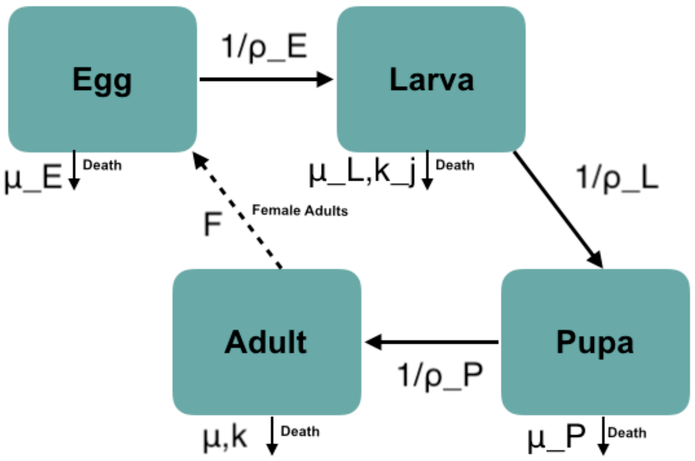
2.1. Dynamical Model of Mosquito Density Including Traits
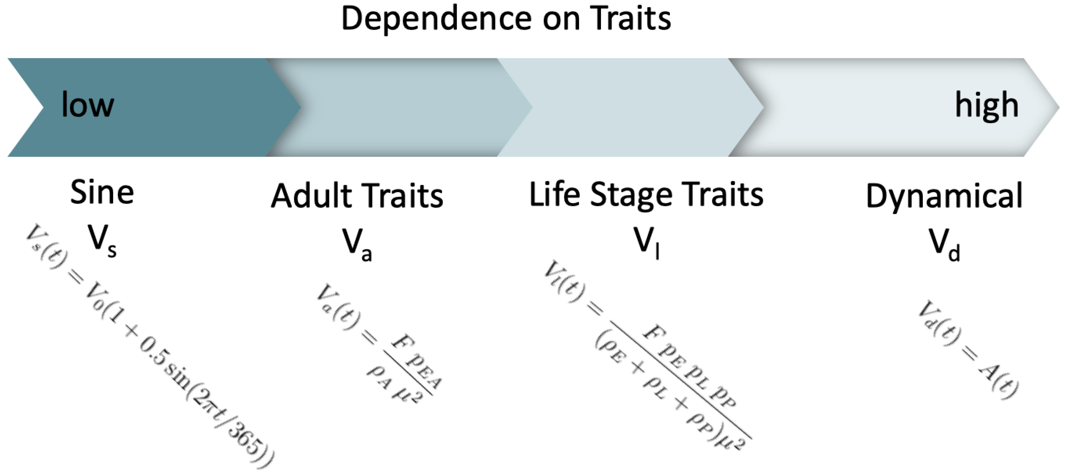
2.2. Alternative Models for Mosquito Density
2.3. Parameterization and Numerical Analysis
3. Results
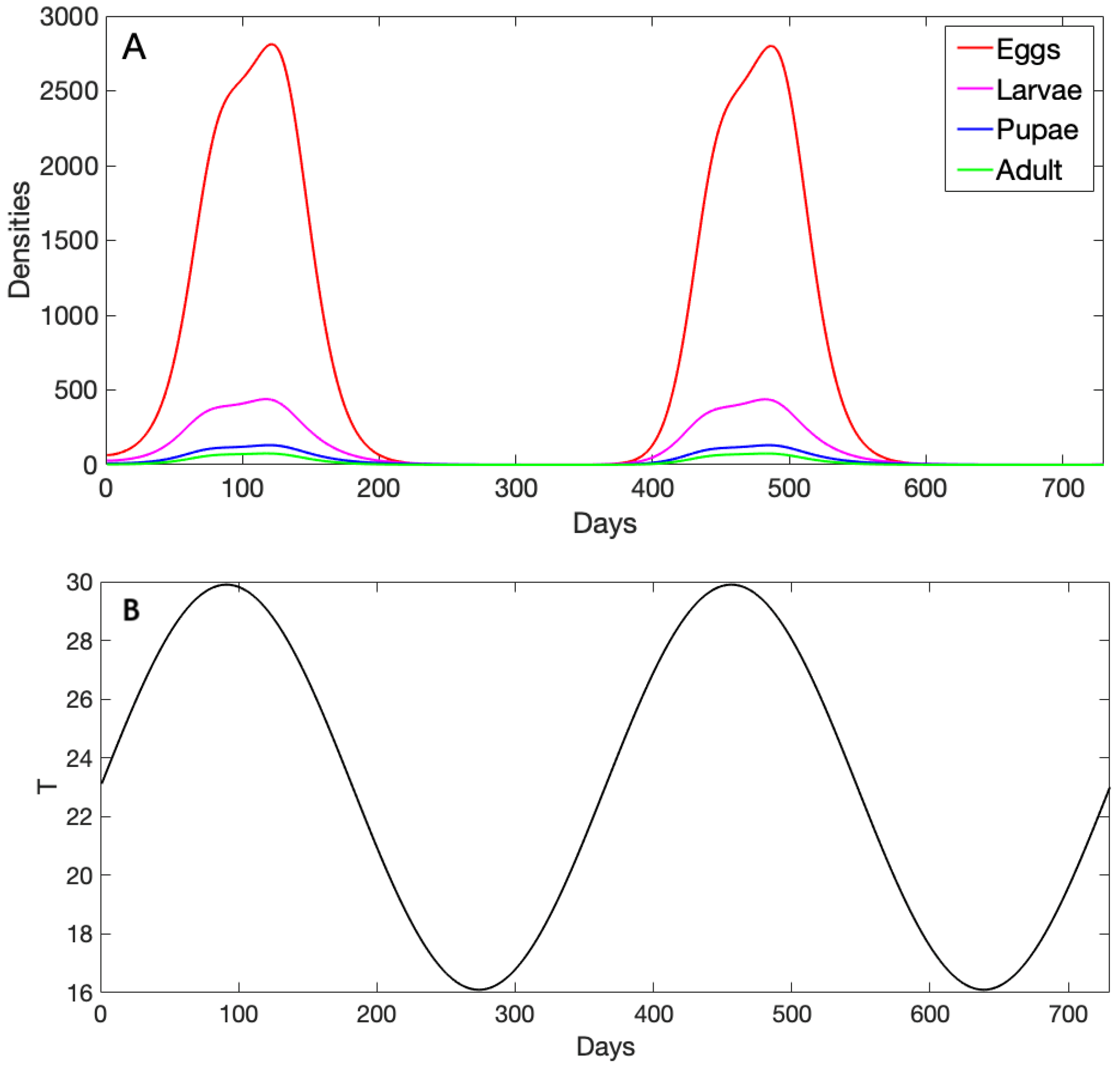
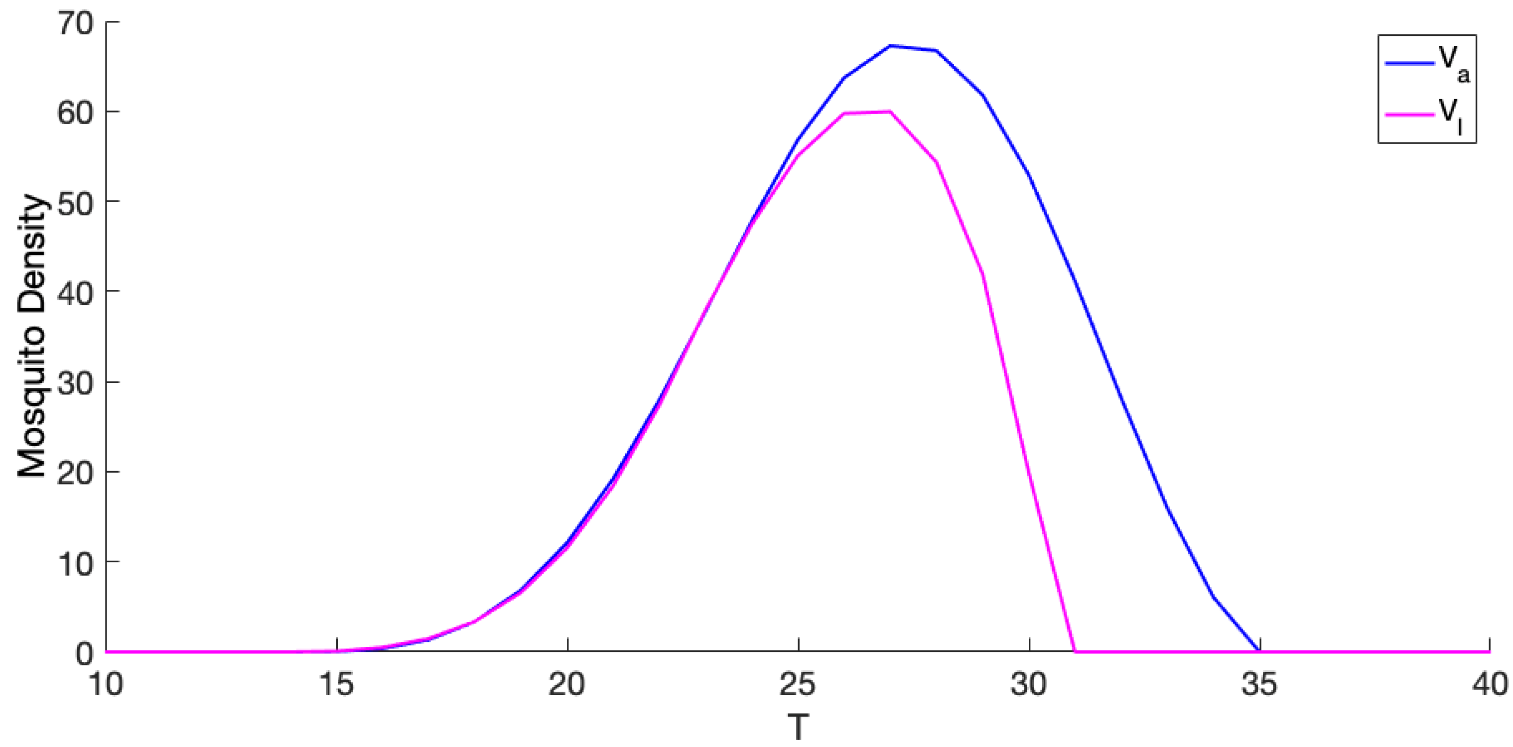
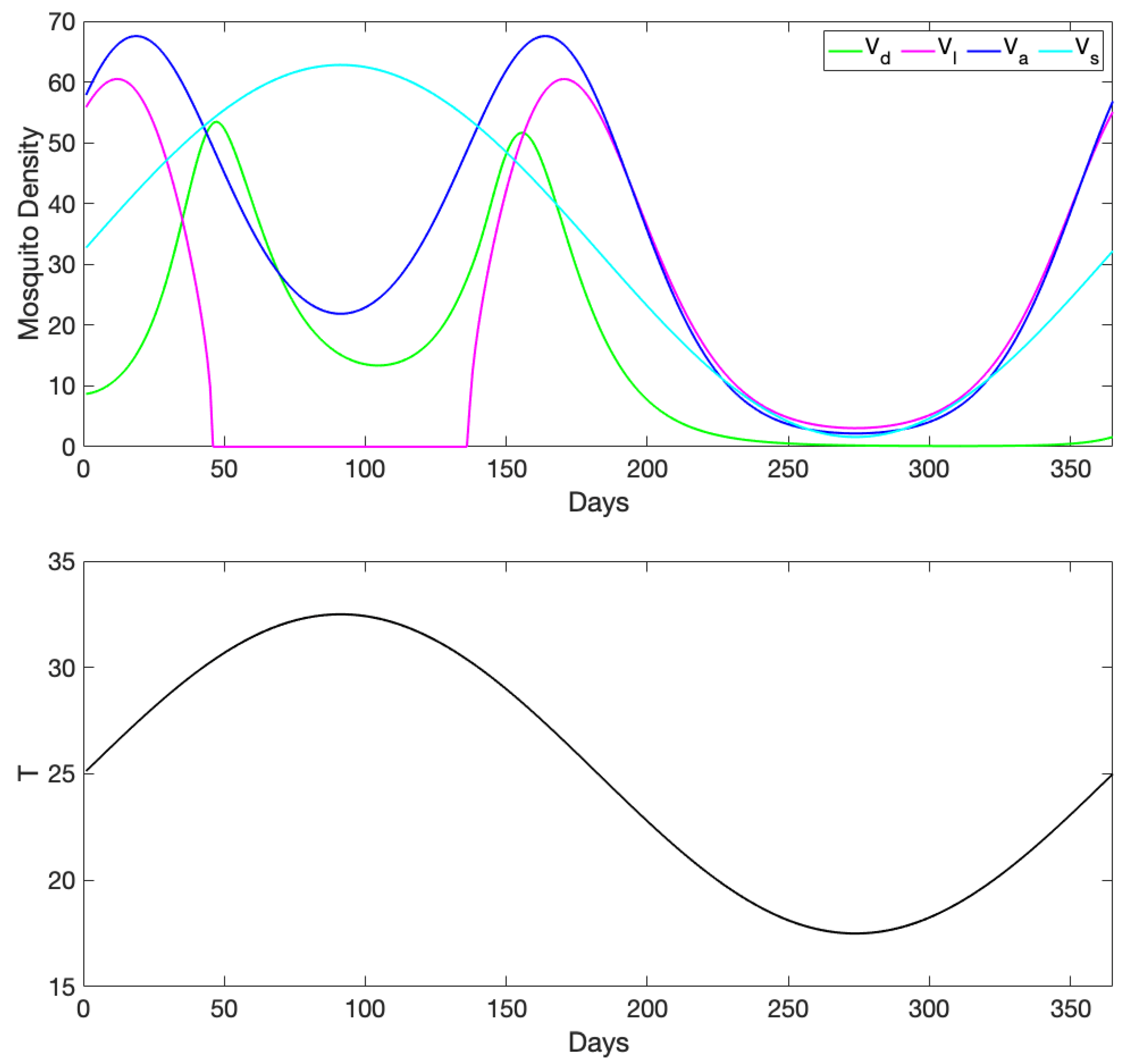
3.1. Exploration of Dynamical Model Behavior
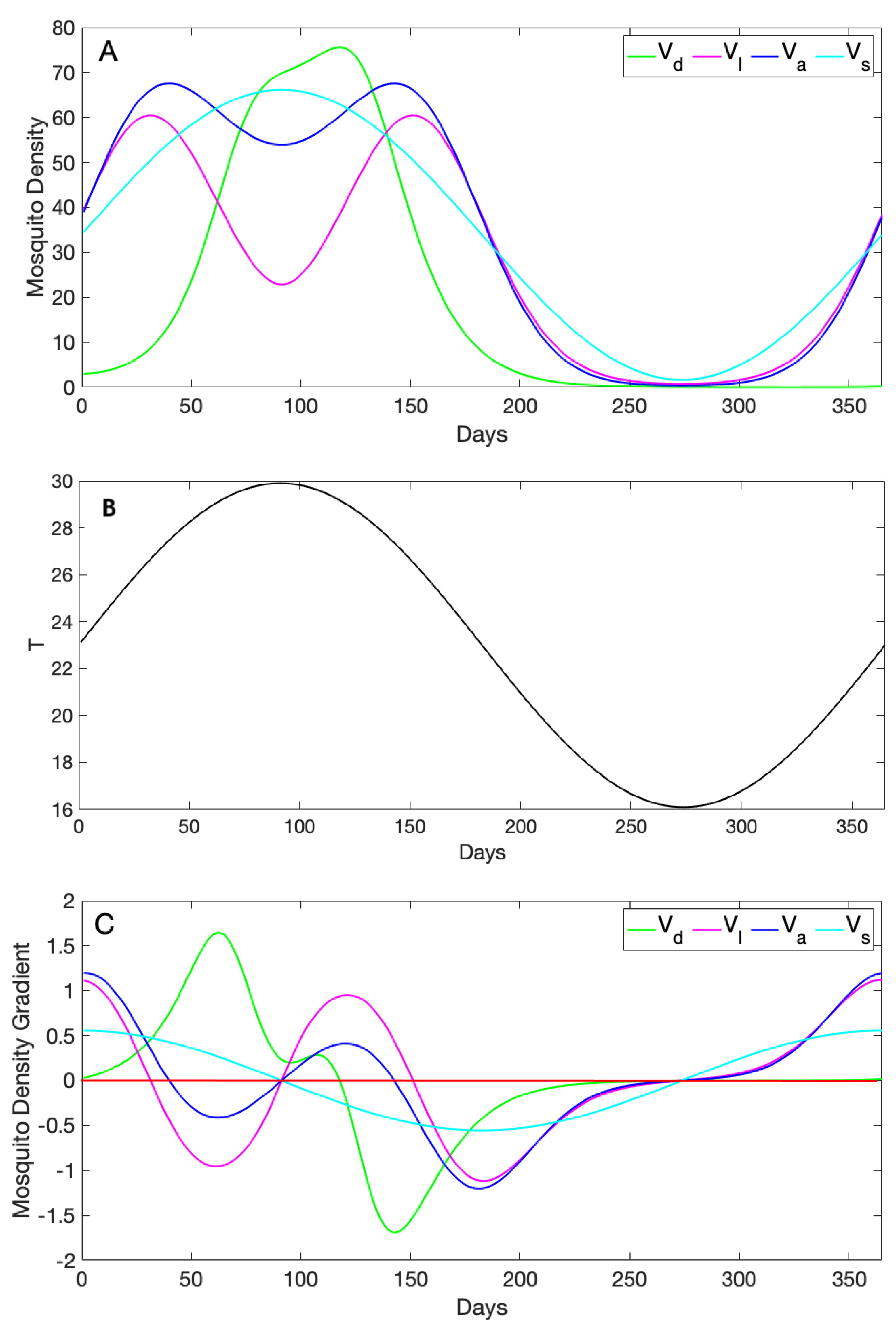
3.2. Comparison of Mosquito Density Patterns across Models
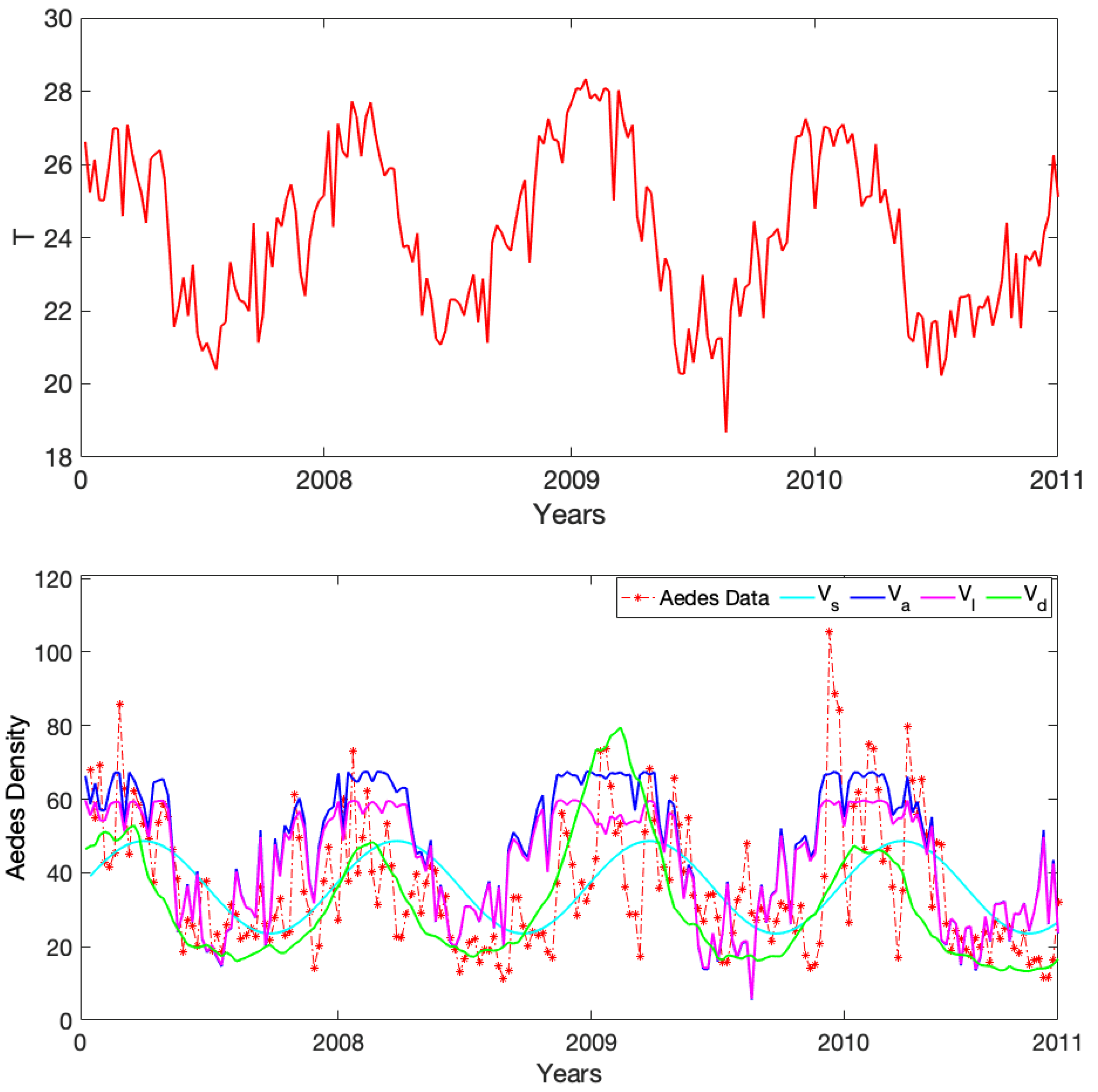
3.3. Comparison to Observational Abundance Data on A. aegypti
4. Discussion
Author Contributions
Funding
Acknowledgments
Conflicts of Interest
Appendix A


References
- The American Mosquito Control Association. The American Mosquito Control Association Report: Mosquito Borne Diseases. The American Mosquito Control Association. Available online: https://www.mosquito.org/page/diseases#Dengue (accessed on 7 November 2019).
- Shaukat, M.A.; Ali, S.; Saddiq, B.; Hassan, M.W.; Ahmad, A.; Kamran, M. Effective Mechanisms to Control Mosquito Borne Diseases: A Review. Am. J. Clin. Neurol. Neurosurg. 2019, 4, 21–30. [Google Scholar]
- Walsh, R.K.; Aguilar, C.L.; Facchinelli, L.; Valerio, L.; Ramsey, J.M.; Scott, T.W.; Lloyd, A.L.; Gould, F. Regulation of Aedes aegypti population dynamics in field systems: Quantifying direct and delayed density dependence. Am. J. Trop. Med. Hyg. 2013, 89, 68–77. [Google Scholar] [CrossRef] [PubMed]
- Dengue Virus Net. Aedes Aegypti, Aedes Albopictus. Dengue Virus Net. Available online: http://www.denguevirusnet.com (accessed on 7 November 2019).
- Scott, T.W.; Morrison, A.C. Vector dynamics and transmission of dengue virus: Implications for dengue surveillance and prevention strategies. In Dengue Virus; Springer: Berlin/Heidelberg, Germany, 2010; pp. 115–128. [Google Scholar]
- Keeling, M.J.; Rohani, P. Modeling Infectious Diseases in Humans and Animals; Princeton University Press: Princeton, NJ, USA, 2011. [Google Scholar]
- Reiner, R.C.; Perkins, T.A.; Barker, C.M.; Niu, T.; Chaves, L.F.; Ellis, A.M.; George, D.B.; Le Menach, A.; Pulliam, J.R.; Bisanzio, D.; et al. A systematic review of mathematical models of mosquito-borne pathogen transmission: 1970–2010. J. R. Soc. Interface 2013, 10, 20120921. [Google Scholar] [CrossRef] [PubMed]
- Robert, M.A.; Christofferson, R.C.; Weber, P.D.; Wearing, H.J. Temperature impacts on dengue emergence in the United States: Investigating the role of seasonality and climate change. Epidemics 2019, 100344. [Google Scholar] [CrossRef] [PubMed]
- Mordecai, E.A.; Paaijmans, K.P.; Johnson, L.R.; Balzer, C.; Ben-Horin, T.; de Moor, E.; McNally, A.; Pawar, S.; Ryan, S.J.; Smith, T.C.; et al. Optimal temperature for malaria transmission is dramatically lower than previously predicted. Ecol. Lett. 2013, 16, 22–30. [Google Scholar] [CrossRef] [PubMed]
- Ryan, S.J.; McNally, A.; Johnson, L.R.; Mordecai, E.A.; Ben-Horin, T.; Paaijmans, K.; Lafferty, K.D. Mapping physiological suitability limits for malaria in Africa under climate change. Vector-Borne Zoonotic Dis. 2015, 15, 718–725. [Google Scholar] [CrossRef]
- Johnson, L.R.; Ben-Horin, T.; Lafferty, K.D.; McNally, A.; Mordecai, E.; Paaijmans, K.P.; Pawar, S.; Ryan, S.J. Understanding uncertainty in temperature effects on vector-borne disease: A Bayesian approach. Ecology 2015, 96, 203–213. [Google Scholar] [CrossRef]
- Brand, S.P.; Rock, K.S.; Keeling, M.J. The interaction between vector life history and short vector life in vector-borne disease transmission and control. PLoS Comput. Biol. 2016, 12, e1004837. [Google Scholar] [CrossRef]
- Achee, N.L.; Gould, F.; Perkins, T.A.; Reiner, R.C., Jr.; Morrison, A.C.; Ritchie, S.A.; Gubler, D.J.; Teyssou, R.; Scott, T.W. A critical assessment of vector control for dengue prevention. PLoS Negl. Trop. Dis. 2015, 9, e0003655. [Google Scholar] [CrossRef]
- Anderson, R.M.; May, R.M. Infectious Diseases of Humans: Dynamics and Control; Oxford University Press: Oxford, UK, 1992. [Google Scholar]
- Lana, R.M.; Morais, M.M.; de Lima, T.F.M.; de Senna Carneiro, T.G.; Stolerman, L.M.; dos Santos, J.P.C.; Cortés, J.J.C.; Eiras, Á.E.; Codeço, C.T. Assessment of a trap based Aedes Aegypti Surveill. Program Using Math. Model. PLoS ONE 2018, 13, e0190673. [Google Scholar] [CrossRef]
- Kraemer, M.U.; Sinka, M.E.; Duda, K.A.; Mylne, A.Q.; Shearer, F.M.; Barker, C.M.; Moore, C.G.; Carvalho, R.G.; Coelho, G.E.; Van Bortel, W.; et al. The global distribution of the arbovirus vectors Aedes aegypti and Ae. albopictus. Elife 2015, 4, e08347. [Google Scholar] [CrossRef] [PubMed]
- CDC. CDC Report: Comparison of Dengue Vectors. CDC. Available online: https://www.cdc.gov/dengue/index.html (accessed on 7 November 2019).
- Bacaër, N. Approximation of the basic reproduction number R 0 for vector-borne diseases with a periodic vector population. Bull. Math. Biol. 2007, 69, 1067–1091. [Google Scholar] [CrossRef] [PubMed]
- Bacaër, N.; Guernaoui, S. The epidemic threshold of vector-borne diseases with seasonality. J. Math. Biol. 2006, 53, 421–436. [Google Scholar] [CrossRef] [PubMed]
- Legros, M.; Lloyd, A.L.; Huang, Y.; Gould, F. Density-dependent intraspecific competition in the larval stage of Aedes aegypti (Diptera: Culicidae): Revisiting the current paradigm. J. Med. Entomol. 2009, 46, 409–419. [Google Scholar] [CrossRef]
- Parham, P.E.; Michael, E. Modeling the effects of weather and climate change on malaria transmission. Environ. Health Perspect. 2010, 118, 620–626. [Google Scholar] [CrossRef]
- Taylor, R.A.; Mordecai, E.A.; Gilligan, C.A.; Rohr, J.R.; Johnson, L.R. Mathematical models are a powerful method to understand and control the spread of Huanglongbing. PeerJ 2016, 4, e2642. [Google Scholar] [CrossRef]
- Taylor, R.A.; Ryan, S.J.; Lippi, C.A.; Hall, D.G.; Narouei-Khandan, H.A.; Rohr, J.R.; Johnson, L.R. Predicting the fundamental thermal niche of crop pests and diseases in a changing world: A case study on citrus greening. J. Appl. Ecol. 2019, 56, 2057–2068. [Google Scholar] [CrossRef]
- Mordecai, E.A.; Cohen, J.M.; Evans, M.V.; Gudapati, P.; Johnson, L.R.; Lippi, C.A.; Miazgowicz, K.; Murdock, C.C.; Rohr, J.R.; Ryan, S.J.; et al. Detecting the impact of temperature on transmission of Zika, dengue, and chikungunya using mechanistic models. PLoS Negl. Trop. Dis. 2017, 11, e0005568. [Google Scholar] [CrossRef]
- Shocket, M.S.; Ryan, S.J.; Mordecai, E.A. Temperature explains broad patterns of Ross River virus transmission. Elife 2018, 7, e37762. [Google Scholar] [CrossRef]
- Messina, J.P.; Brady, O.J.; Golding, N.; Kraemer, M.U.; Wint, G.W.; Ray, S.E.; Pigott, D.M.; Shearer, F.M.; Johnson, K.; Earl, L.; et al. The current and future global distribution and population at risk of dengue. Nat. Microbiol. 2019, 4, 1508–1515. [Google Scholar] [CrossRef]
- Honório, N.A.; Nogueira, R.M.R.; Codeço, C.T.; Carvalho, M.S.; Cruz, O.G.; Magalhães, M.D.A.F.M.; de Araújo, J.M.G.; de Araújo, E.S.M.; Gomes, M.Q.; Pinheiro, L.S.; et al. Spatial evaluation and modeling of dengue seroprevalence and vector density in Rio de Janeiro, Brazil. PLoS Negl. Trop. Dis. 2009, 3, e545. [Google Scholar] [CrossRef] [PubMed]
- Liu-Helmersson, J.; Brännström, Å.; Sewe, M.O.; Semenza, J.C.; Rocklöv, J. Estimating Past, Present, and Future Trends in the Global Distribution and Abundance of the Arbovirus Vector Aedes aegypti Under Climate Change Scenarios. Front. Public Health 2019, 7. [Google Scholar] [CrossRef] [PubMed]
- Koyoc-Cardeña, E.; Medina-Barreiro, A.; Cohuo-Rodríguez, A.; Pavía-Ruz, N.; Lenhart, A.; Ayora-Talavera, G.; Dunbar, M.; Manrique-Saide, P.; Vazquez-Prokopec, G. Estimating absolute indoor density of Aedes aegypti using removal sampling. Parasites Vectors 2019, 12, 250. [Google Scholar] [CrossRef] [PubMed]
- Lana, R.M.; Carneiro, T.G.; Honório, N.A.; Codeço, C.T. Seasonal and nonseasonal dynamics of Aedes Aegypti Rio De Janeiro, Brazil: Fitting mathematical models to trap data. Acta Trop. 2014, 129, 25–32. [Google Scholar] [CrossRef]
- Lana, R.M.; da Costa Gomes, M.F.; de Lima, T.F.M.; Honório, N.A.; Codeço, C.T. The introduction of dengue follows transportation infrastructure changes in the state of Acre, Brazil: A network-based analysis. PLoS Negl. Trop. Dis. 2017, 11, e0006070. [Google Scholar] [CrossRef]
- Morin, C.W.; Monaghan, A.J.; Hayden, M.H.; Barrera, R.; Ernst, K. Meteorologically driven simulations of dengue epidemics in San Juan, PR. PLoS Negl. Trop. Dis. 2015, 9, e0004002. [Google Scholar] [CrossRef]
- Rueda, L.; Patel, K.; Axtell, R.; Stinner, R. Temperature-dependent development and survival rates of Culex quinquefasciatus and Aedes Aegypti (Diptera: Culicidae). J. Med. Entomol. 1990, 27, 892–898. [Google Scholar] [CrossRef]
- Mohammed, A.; Chadee, D.D. Effects of different temperature regimens on the development of Aedes Aegypti (L.) (Diptera: Culicidae) Mosquitoes. Acta Trop. 2011, 119, 38–43. [Google Scholar] [CrossRef]


| Parameter | Description | Function | Value | Units |
|---|---|---|---|---|
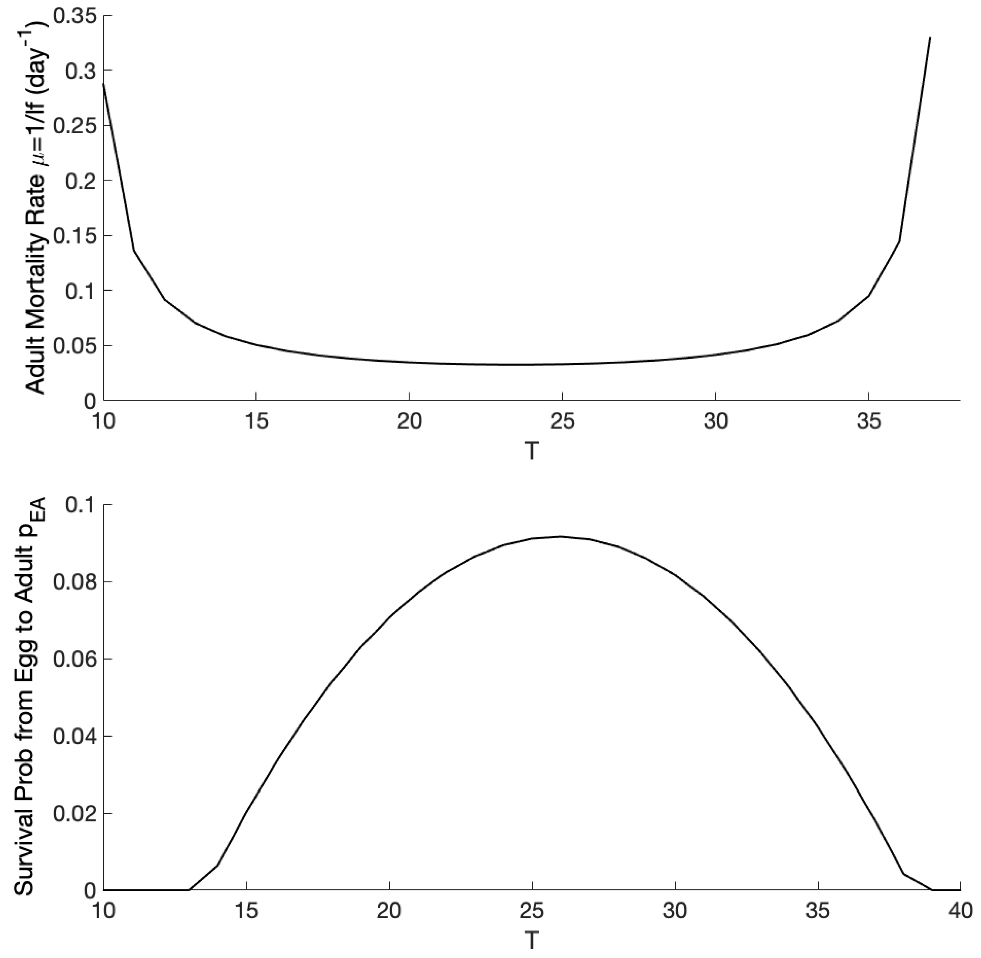
| Adult mosquito lifespan () | quad | day | ||
| Eggs-to-adult survival probability | quad | - | ||
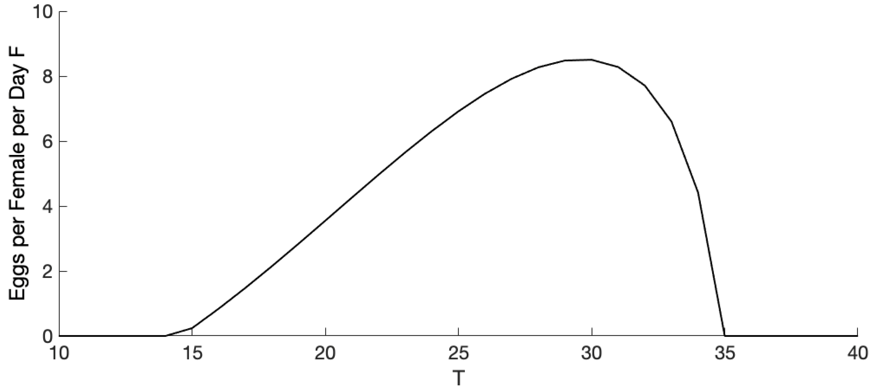
| F | Eggs per female per day | Brière | day−1 | |
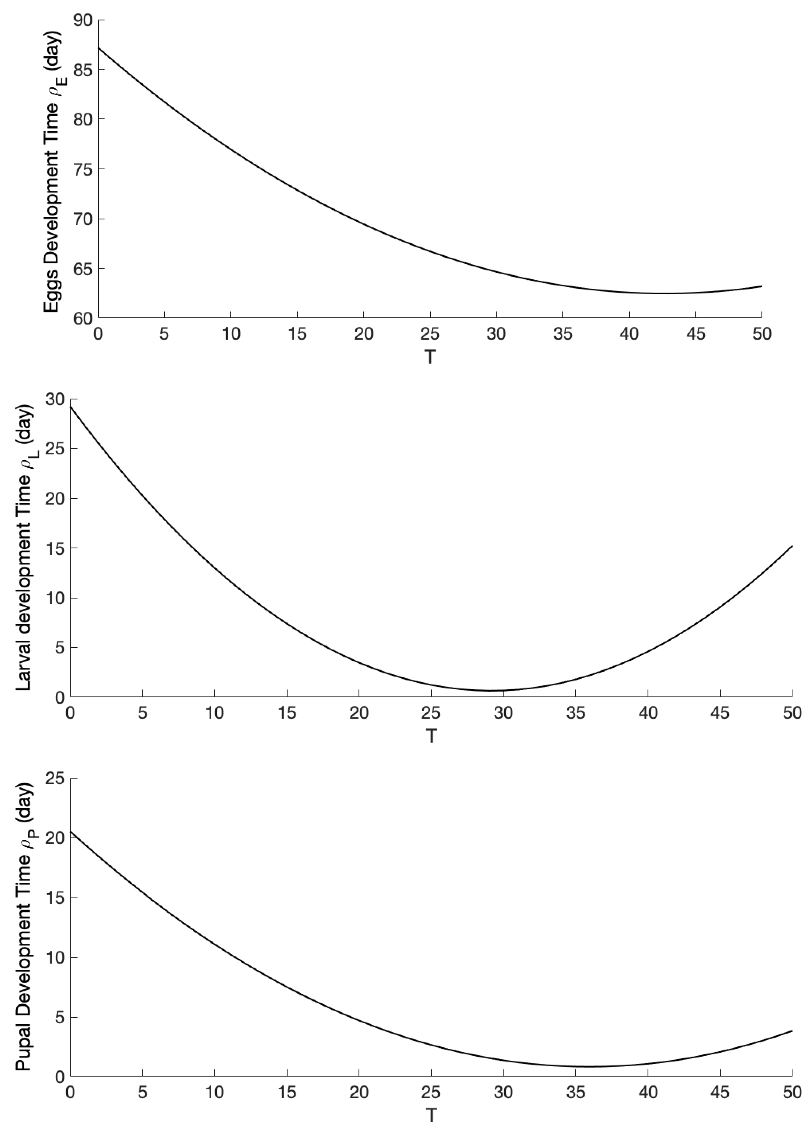
| Eggs development time | quad | day | ||
| Larval development time | quad | day | ||
| Pupal development time | quad | day | ||
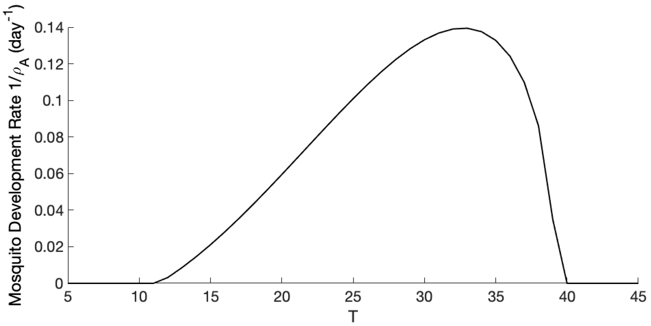
| Mosquito development rate | Brière | day−1 | ||
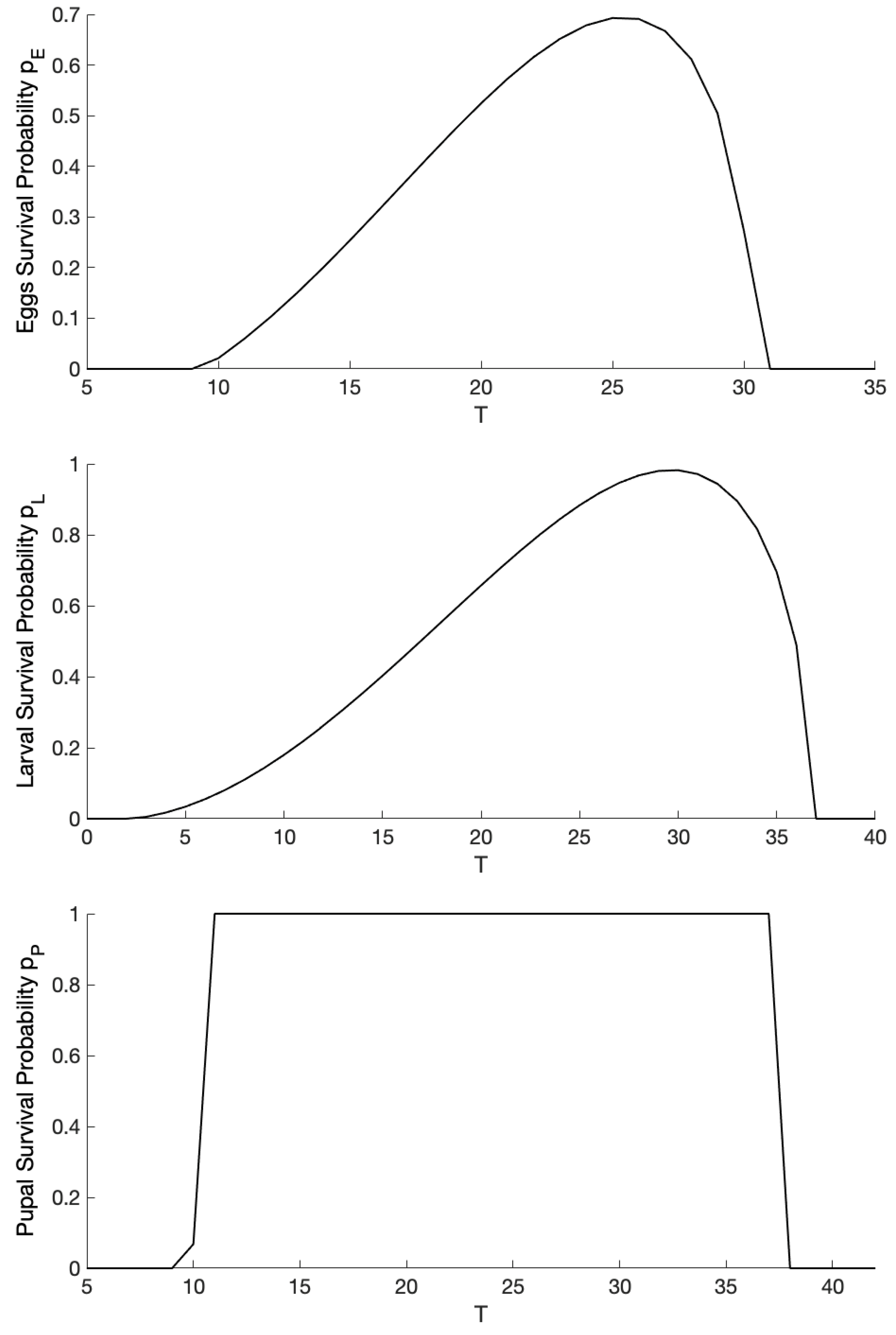
| Eggs survival probability | Brière | - | ||
| Larval survival probability | Brière | - | ||
| Pupal survival probability | Brière | - | ||
| k | Temperature-independent mortality rate | - | 0.486 | day−1 |
| Density-dependent mortality rate | - | 0.09 | day−1 |
| Model | ||||
|---|---|---|---|---|
| MSE | 279 | 255 | 316 | 227 |
© 2019 by the authors. Licensee MDPI, Basel, Switzerland. This article is an open access article distributed under the terms and conditions of the Creative Commons Attribution (CC BY) license (http://creativecommons.org/licenses/by/4.0/).
Share and Cite
El Moustaid, F.; Johnson, L.R. Modeling Temperature Effects on Population Density of the Dengue Mosquito Aedes aegypti. Insects 2019, 10, 393. https://doi.org/10.3390/insects10110393
El Moustaid F, Johnson LR. Modeling Temperature Effects on Population Density of the Dengue Mosquito Aedes aegypti. Insects. 2019; 10(11):393. https://doi.org/10.3390/insects10110393
Chicago/Turabian StyleEl Moustaid, Fadoua, and Leah R. Johnson. 2019. "Modeling Temperature Effects on Population Density of the Dengue Mosquito Aedes aegypti" Insects 10, no. 11: 393. https://doi.org/10.3390/insects10110393
APA StyleEl Moustaid, F., & Johnson, L. R. (2019). Modeling Temperature Effects on Population Density of the Dengue Mosquito Aedes aegypti. Insects, 10(11), 393. https://doi.org/10.3390/insects10110393