Evaluation of NEON Data to Model Spatio-Temporal Tick Dynamics in Florida


Abstract
:1. Introduction
2. Methods
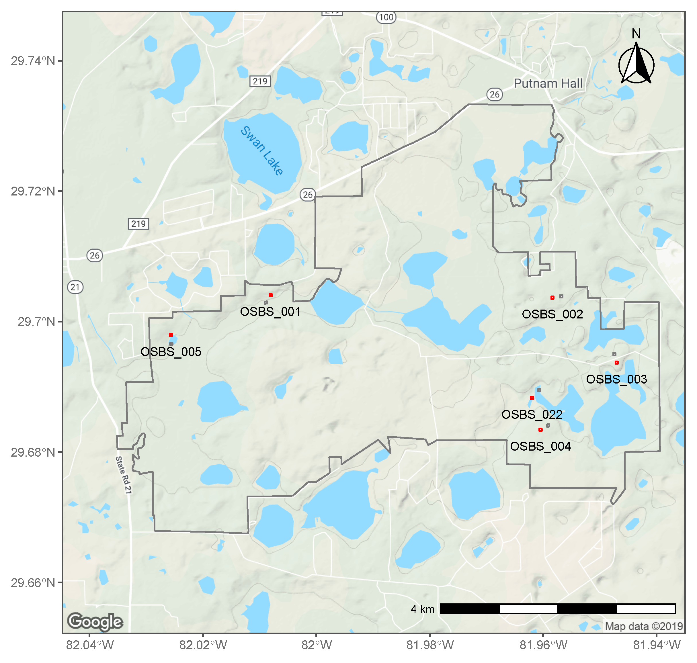
2.1. NEON Data
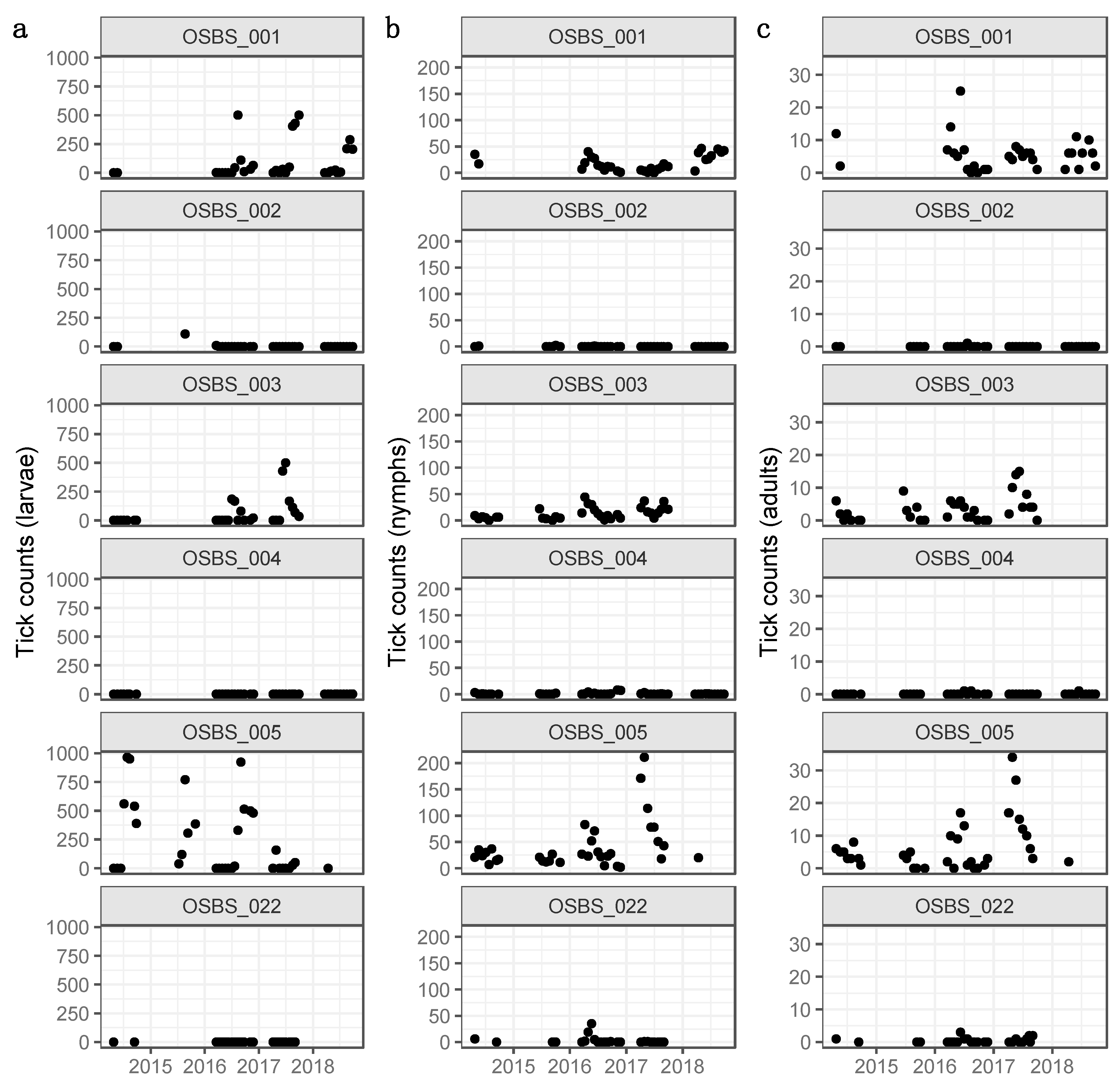
2.2. Tick Counts
2.3. Precipitation
2.4. Relative Humidity
2.5. Temperature
2.6. Woody Plant Vegetation Structure
2.7. Herbaceous Vegetation
2.8. Biodiversity and Non-Vegetative Cover
2.9. Abundance Modeling: N-Mixture Models
2.10. Software Used, Data and Code Availability
3. Results
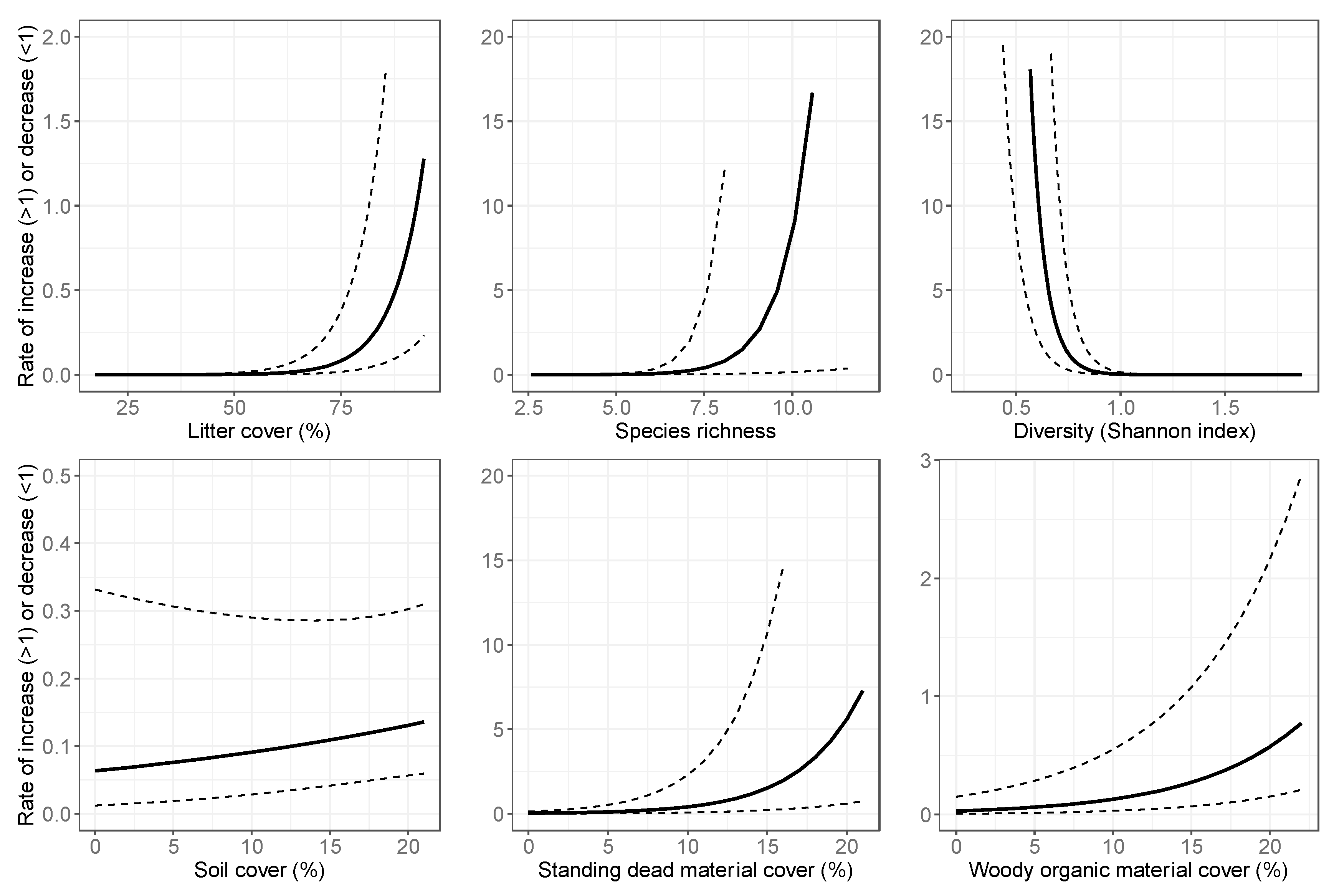
3.1. Distributions, Change Dynamics and Explanatory Variables
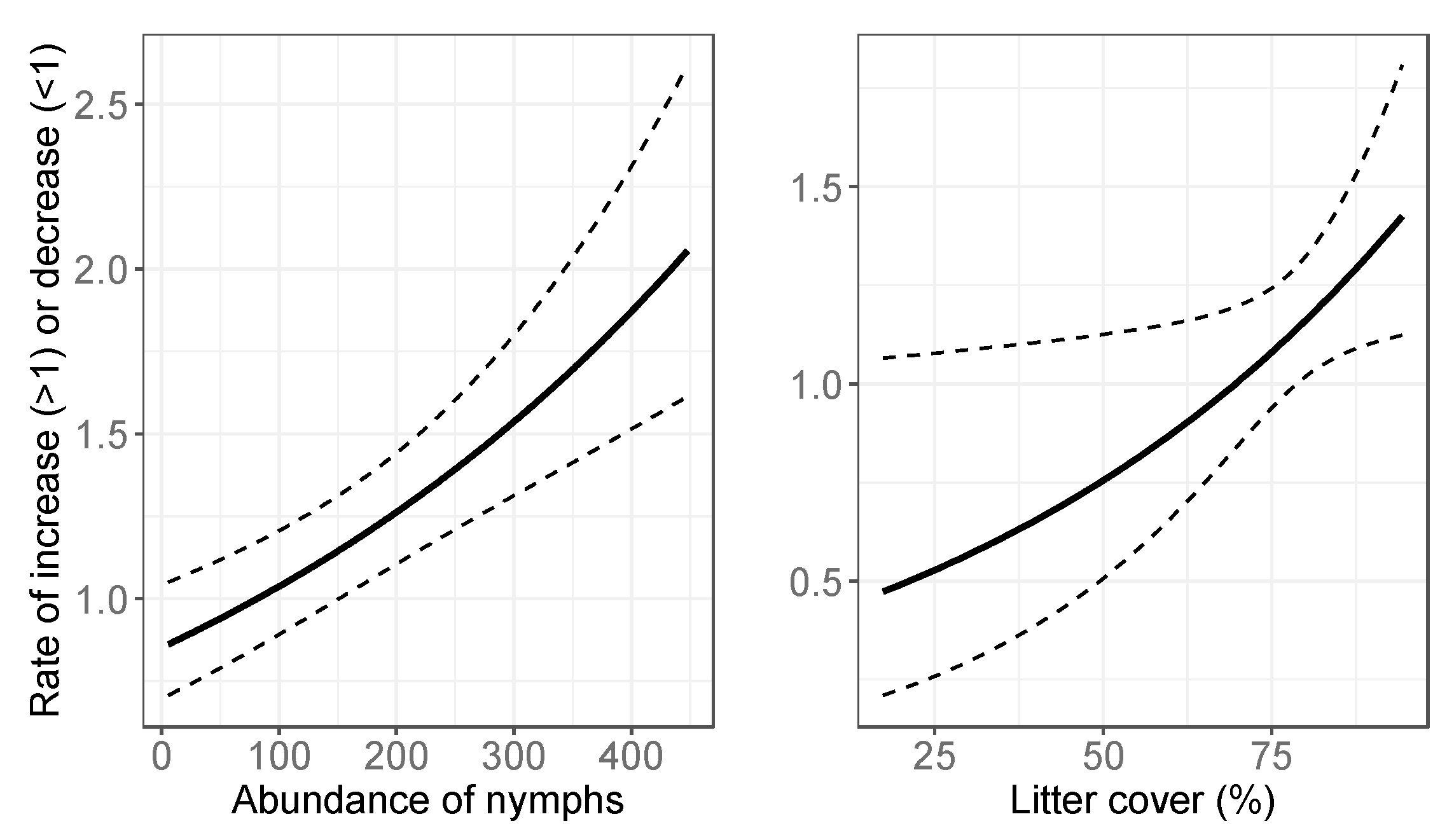
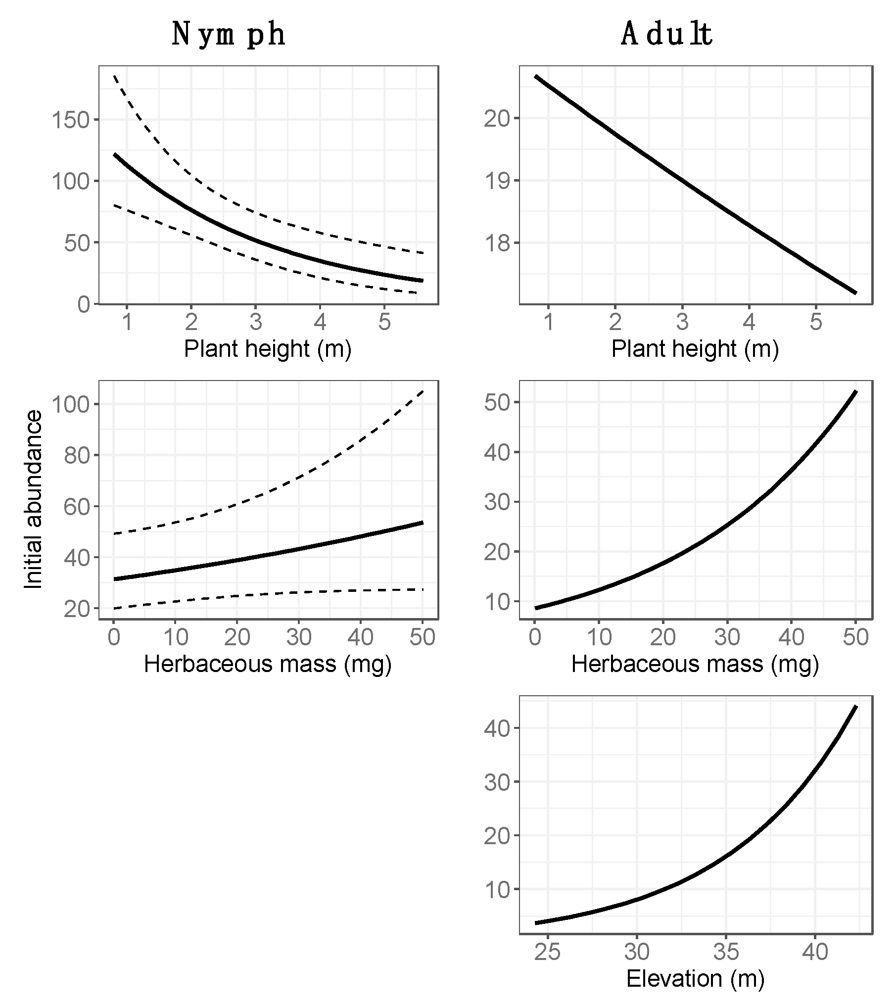
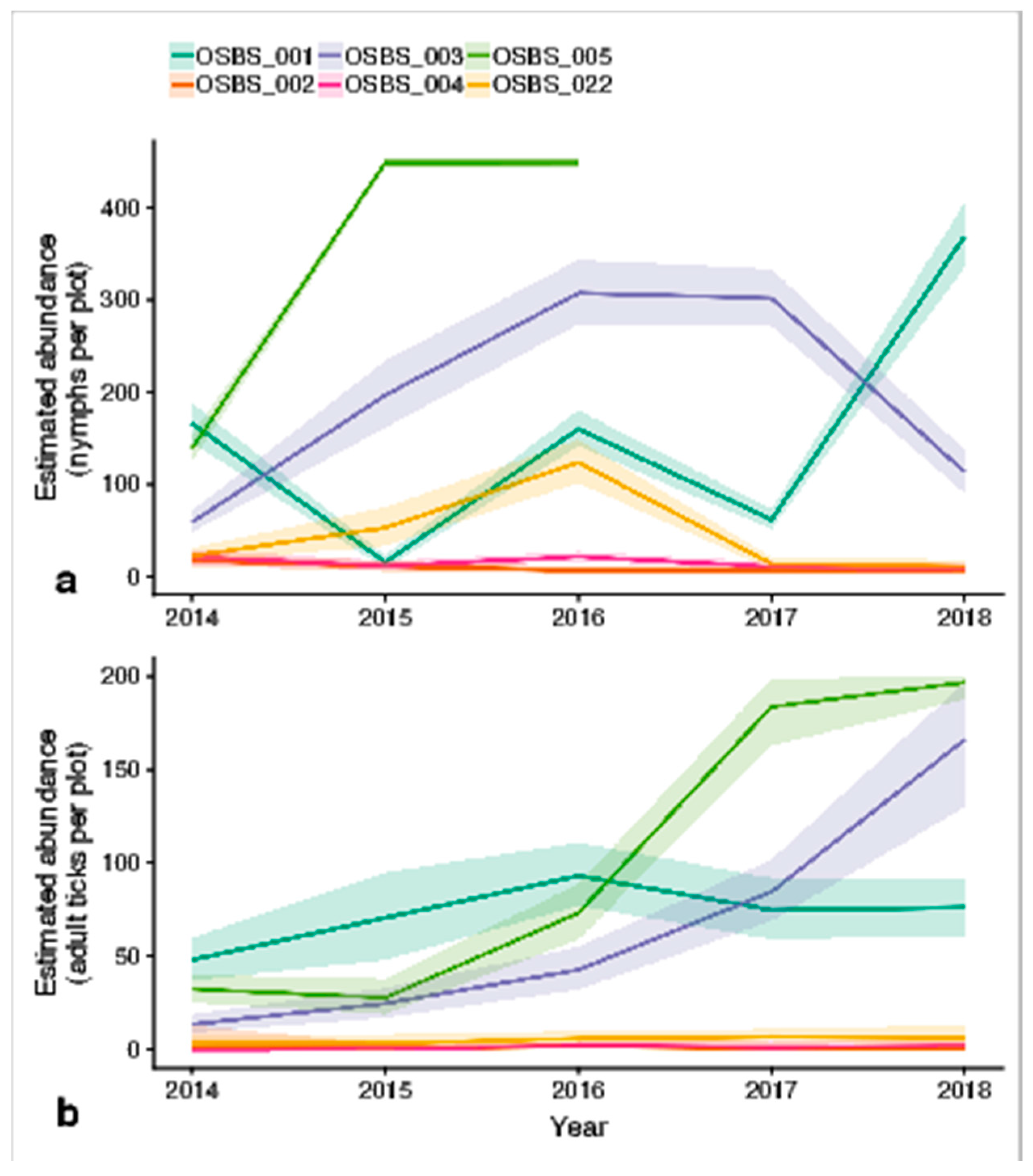
3.2. Final Models: Abundance Estimates
4. Discussion
4.1. Spatial Variation in Abundance
4.2. Temporal Variation in Abundance
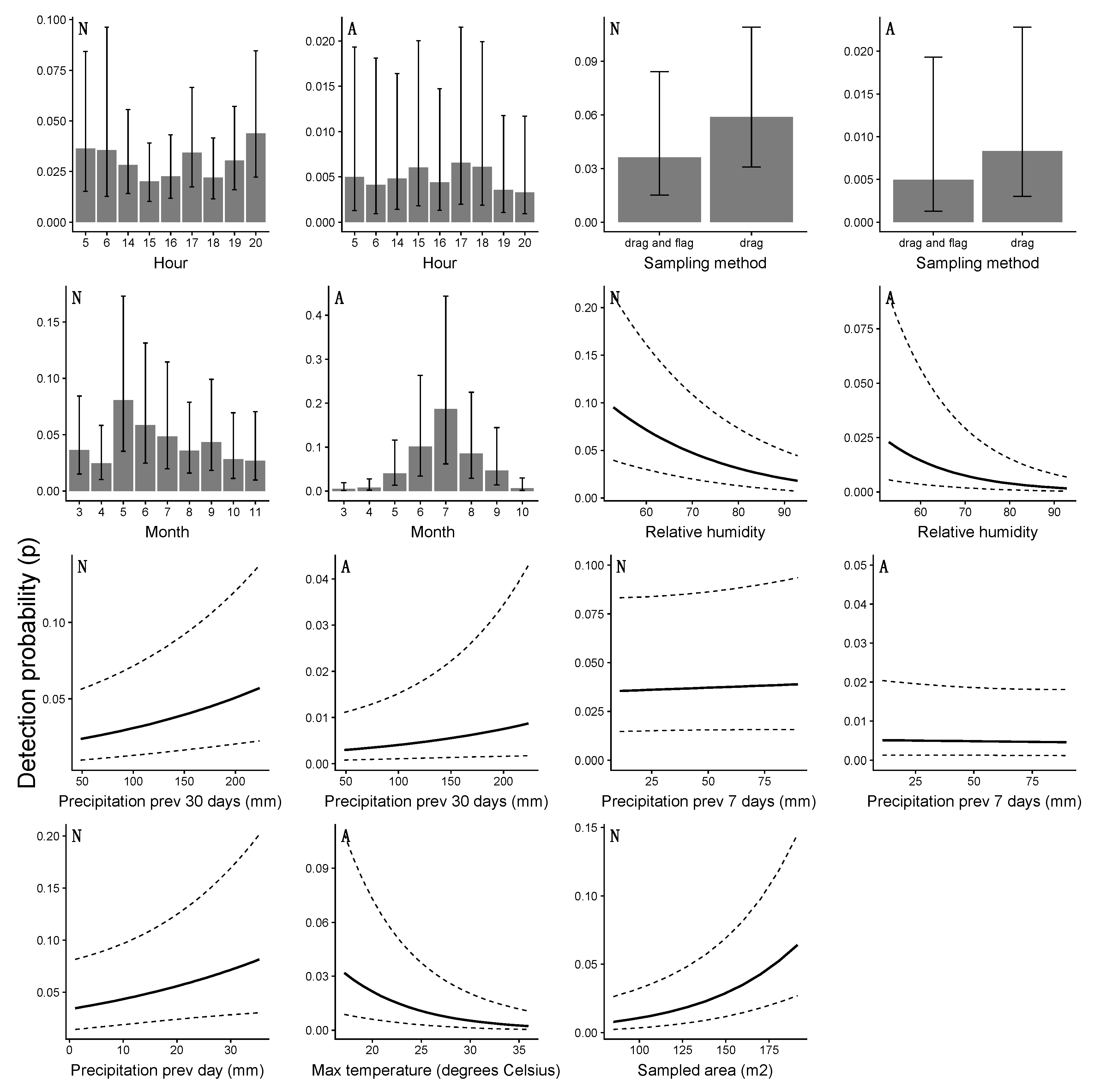
4.3. Detection Probability and the Risk of Human Exposure
5. Conclusions
Supplementary Materials
Author Contributions
Funding
Acknowledgments
Conflicts of Interest
References
- Bradley, C.A.; Rolka, H.; Walker, D.; Loonsk, J. Implementation of laboratory order data in BioSense Early Event Detection and Situation Awareness System. MMWR Morb. Mortal. Wkly. Rep. 2005, 54 (Suppl. S1), 11–19. [Google Scholar]
- Jongejan, F.; Uilenberg, G. The global importance of ticks. Parasitology 2005, 129, S3–S14. [Google Scholar] [CrossRef] [PubMed]
- Sonenshine, D. Range Expansion of Tick Disease Vectors in North America: Implications for Spread of Tick-Borne Disease. IJERPH 2018, 15, 478. [Google Scholar] [CrossRef] [PubMed]
- Rand, P.W.; Lubelczyk, C.; Lavigne, G.R.; Elias, S.; Holman, M.S.; Lacombe, E.H.; Smith, R.P., Jr. Deer Density and the Abundance of Ixodes scapularis (Acari: Ixodidae). J. Med. Entomol. 2003, 179–184. [Google Scholar] [CrossRef] [PubMed]
- Barna, M. US Cases of Tick-Borne Diseases on the Rise. Am. J. Public Health 2019, 109, 951. [Google Scholar]
- Centers for Disease Control and Prevention. Available online: https://www.cdc.gov/ticks/surveillance/index.html (accessed on 29 July 2019).
- Springer, Y.P.; Hoekman, D.; Johnson, P.T.J.; Duffy, P.A.; Hufft, R.A.; Barnett, D.T.; Allan, B.F.; Amman, B.R.; Barker, C.M.; Barrera, R.; et al. Tick-, mosquito-, and rodent-borne parasite sampling designs for the National Ecological Observatory Network. Ecosphere 2016, 7, e01271. [Google Scholar] [CrossRef]
- Arsnoe, I.M.; Hickling, G.J.; Ginsberg, H.S.; McElreath, R.; Tsao, J.I. Different Populations of Blacklegged Tick Nymphs Exhibit Differences in Questing Behavior That Have Implications for Human Lyme Disease Risk. PLoS ONE 2015, 10, e0127450. [Google Scholar] [CrossRef]
- Keller, M.; Schimel, D.S.; Hargrove, W.W.; Hoffman, F.M. A continental strategy for the National Ecological Observatory Network. Front. Ecol. Environ. 2008, 6, 282–284. [Google Scholar] [CrossRef]
- Thorpe, A.S.; Barnett, D.T.; Elmendorf, S.C.; Hinckley, E.-L.S.; Hoekman, D.; Jones, K.D.; LeVan, K.E.; Meier, C.L.; Stanish, L.F.; Thibault, K.M. Introduction to the sampling designs of the National Ecological Observatory Network Terrestrial Observation System. Ecosphere 2016, 7, e01627. [Google Scholar] [CrossRef]
- National Ecological Observatory Network Provisional. Available online: http://data.neonscience.org (accessed on 8 March 2019).
- Tsao, K.; Thibault, K.; LeVan, K.; Springer, Y. TOS Protocol and Procedure: Tick and Tick-Borne Pathogen Sampling, Revision H; NEON: Boulder, CO, USA, 2017. [Google Scholar]
- Meier, C.; Jones, K. TOS Science Design for Plant Biomass, Productivity, and Leaf Area Index, Revision A; NEON: Boulder, CO, USA, 2014. [Google Scholar]
- Meier, C.; Jones, K. TOS Protocol and Procedure: Measurement of Vegetation Structure, Revision G; NEON: Boulder, CO, USA, 2017. [Google Scholar]
- Meier, C.; Chesney, T.; Jones, K. NEON User Guide to Woody Plant Vegetation Structure (NEON.DP1.10098) and Non-Herbaceous Perennial Vegetation Structure (NEON.DP1.10045), Revision A; NEON: Boulder, CO, USA, 2018. [Google Scholar]
- Tomascik, T.; Sander, F. Effects of eutrophication on reef-building corals. Mar. Biol. 1987, 94, 53–75. [Google Scholar] [CrossRef]
- MacKenzie, D.I.; Nichols, J.D.; Lachman, G.B.; Droege, S.; Andrew Royle, J.; Langtimm, C.A. Estimating site occupancy rates when detection probabilities are less than one. Ecology 2002, 83, 2248–2255. [Google Scholar] [CrossRef]
- Kery, M.; Royle, J.A.; Schmid, H. Modeling avian abundance from replicated counts using binomial mixture models. Ecol. Appl. 2005, 15, 1450–1461. [Google Scholar] [CrossRef]
- Hostetler, J.A.; Chandler, R.B. Improved state-space models for inference about spatial and temporal variation in abundance from count data. Ecology 2015, 96, 1713–1723. [Google Scholar] [CrossRef]
- Royle, J.A. N-Mixture models for estimating population size from spatially replicated counts. Biometrics 2004, 60, 108–115. [Google Scholar] [CrossRef] [PubMed]
- Kery, M.; Dorazio, R.M.; Soldaat, L.; Van Strien, A.; Zuiderwijk, A.; Royle, J.A. Trend estimation in populations with imperfect detection. J. Appl. Ecol. 2009, 46, 1163–1172. [Google Scholar] [CrossRef]
- Dail, D.; Madsen, L. Models for Estimating Abundance from Repeated Counts of an Open Metapopulation. Biometrics 2011, 67, 577–587. [Google Scholar] [CrossRef]
- Ricker, W.E. Stock and Recruitment. J. Fish. Res. Board Can. 1954, 11, 559–623. [Google Scholar] [CrossRef]
- Hart, E.M.; Gotelli, N.J. The effects of climate change on density-dependent population dynamics of aquatic invertebrates. Oikos 2011, 120, 1227–1234. [Google Scholar] [CrossRef]
- Fiske, I.; Chandler, R. unmarked: An RPackage for Fitting Hierarchical Models of Wildlife Occurrence and Abundance. J. Stat. Softw. 2011, 43, 23. [Google Scholar] [CrossRef]
- Akaike, H. Information Theory and an Extension of the Maximum Likelihood Principle. In Selected Papers of Hirotugu Akaike; Selected Papers of Hirotugu Akaike; Parzen, E., Tanabe, K., Kitagawa, G., Eds.; Springer: New York, NY, USA, 1998; pp. 199–213. [Google Scholar]
- Burnham, K.P.; Anderson, D.R. Model Selection and Multimodel Inference: A Practical Information-theoretic Approach; Springer: New York, NY, USA, 2002; pp. 1–515. [Google Scholar]
- Royle, J.A.; Nichols, J.D. Estimating abundance from repeated presence-absence data or count points. Ecology 2003, 84, 777–790. [Google Scholar] [CrossRef]
- R Core Team. R: A Language and Environment for Statistical Computing; R Foundation for Statistical Computing: Vienna, Austria, 2017. [Google Scholar]
- Fiske, I. Overview of Unmarked: An R Package for the Analysis of Data from Unmarked Animals; CRAN: Vienna, Austria, 2017. [Google Scholar]
- Fiske, I.; Chandler, R.; Miller, D.; Royle, A.; Kery, M.; Hostetler, J.; Hutchinson, R. Package “Unmarked”: Models for Data from Unmarked Animals; Version 0.12-2; CRAN: Vienna, Austria, 2017. [Google Scholar]
- Kery, M. Identifiability in N-mixture models: A large-scale screening test with bird data. Ecology 2018, 99, 281–288. [Google Scholar] [CrossRef]
- Gleim, E.R.; Conner, L.M.; Berghaus, R.D.; Levin, M.L.; Zemtsova, G.E.; Yabsley, M.J. The Phenology of Ticks and the Effects of Long-Term Prescribed Burning on Tick Population Dynamics in Southwestern Georgia and Northwestern Florida. PLoS ONE 2014, 9, e112174. [Google Scholar] [CrossRef]
- Prusinski, M.A.; Chen, H.; Drobnack, J.M.; Kogut, S.J.; Means, R.G.; Howard, J.J.; Oliver, J.; Lukacik, G.; Backenson, P.B.; White, D.J. Habitat Structure Associated with Borrelia burgdorferi Prevalence in Small Mammals in New York State. Environ. Entomol. 2006, 35, 308–319. [Google Scholar] [CrossRef]
- Chesney, T.; Thibault, K. NEON User Guide to Small Mammal Box Trapping (NEON.DP1.10072), Revision A; NEON: Boulder, CO, USA, 2018. [Google Scholar]
- Thibault, K.M.; Tsao, K.; Springer, Y.; Knapp, L. TOS Protocol and Procedure: Small Mammal Sampling, Revision L; NEON: Boulder, CO, USA, 2019. [Google Scholar]
- Rota, C.T.; Ferreira, M.A.R.; Kays, R.W.; Forrester, T.D.; Kalies, E.L.; McShea, W.J.; Parsons, A.W.; Millspaugh, J.J. A multispecies occupancy model for two or more interacting species. Methods Ecol. Evol. 2016, 7, 1164–1173. [Google Scholar] [CrossRef]
- Gomez, J.P.; Robinson, S.K.; Blackburn, J.K.; Ponciano, J.M. An efficient extension of N-mixture models for multi-species abundance estimation. Methods Ecol. Evol. 2017, 9, 340–353. [Google Scholar] [CrossRef]
- Barnett, D.T. TOS Protocol and Procedure: Plant Diversity Sampling, Revision G; NEON: Boulder, CO, USA, 2017. [Google Scholar]
- Springer, Y.P.; Jarnevich, C.S.; Monaghan, A.J.; Eisen, R.J.; Barnett, D.T. Modeling the Present and Future Geographic Distribution of the Lone Star Tick, Amblyomma americanum (Ixodida: Ixodidae), in the Continental United States. Am. J. Trop. Med. Hyg. 2015, 93, 875–890. [Google Scholar] [CrossRef]
- Stephenson, N.; Wong, J.; Foley, J. Host, habitat and climate preferences of Ixodes angustus (Acari: Ixodidae) and infection with Borrelia burgdorferi and Anaplasma phagocytophilum in California, USA. Exp. Appl. Acarol. 2016, 70, 239–252. [Google Scholar] [CrossRef]
- Fryxell, R.T.T.; Moore, J.E.; Collins, M.D.; Kwon, Y.; Jean-Philippe, S.R.; Schaeffer, S.M.; Odoi, A.; Kennedy, M.; Houston, A.E. Habitat and Vegetation Variables Are Not Enough When Predicting Tick Populations in the Southeastern United States. PLoS ONE 2015, 10, e0144092. [Google Scholar]
- Ginsberg, H.S.; Ewing, C.P. Comparison of Flagging, Walking, Trapping, and Collecting from Hosts as Sampling Methods for Northern Deer Ticks. Exp. Appl. Acarol. 1989, 7, 313–322. [Google Scholar] [CrossRef]
- Glass, G.E.; Ganser, C.; Wisely, S.M.; Kessler, W.H. Kessler Standardized Ixodid Tick Survey in Mainland Florida. Insects 2019, 10, 235. [Google Scholar] [CrossRef]
- Mejlon, H.A.; Jaenson, T.G.T. Questing behaviour of Ixodes ricinus ticks (Acari: Ixodidae). Exp. Appl. Acarol. 1997, 747–754. [Google Scholar] [CrossRef]
- Berger, K.A.; Ginsberg, H.S.; Gonzalez, L.; Mather, T.N. Relative Humidity and Activity Patterns of Ixodes scapularis(Acari: Ixodidae). J. Med. Entomol. 2014, 51, 769–776. [Google Scholar] [CrossRef]
- Tack, W.; Madder, M.; De Frenne, P.; Vanhellemont, M.; Gruwez, R.; Verheyen, K. The effects of sampling method and vegetation type on the estimated abundance of Ixodes ricinus ticks in forests. Exp. Appl. Acarol. 2011, 54, 285–292. [Google Scholar] [CrossRef]


| Data Product ID | Product Name | Site ID | Date Range |
|---|---|---|---|
| DP1.10093.001 | Tick sampling | OSBS | 1 January 2013–31 December 2018 |
| DP1.10098.001 | Woody plant vegetation structure | OSBS | 1 January 2013–31 December 2018 |
| DP1.10058.001 | Plant presence and percent cover | OSBS | 1 January 2013–31 December 2018 |
| DP1.10072.001 | Small mammal box trapping | OSBS | 1 January 2013–31 December 2018 |
| DP1.10023.001 | Herbaceous clip harvest | OSBS | 1 January 2013–31 December 2018 |
| DP1.00006.001 | Precipitation (tower) | OSBS | 1 January 2013–31 December 2018 |
| DP1.00098.001 | Relative humidity (tower) | OSBS | 1 January 2013–31 December 2018 |
| DP1.00002.001 | Single aspirated air temperature (tower) | OSBS | 1 January 2013–31 December 2018 |
| Nymphs | Adults | ||||
|---|---|---|---|---|---|
| Distribution | Dynamics | AIC | Distribution | Dynamics | AIC |
| NB | Trend | 2832 | NB | Trend | 909 |
| NB | Autoregressive | 2834 | NB | Gompertz | 910 |
| NB | Gompertz | 2870 | NB | Autoregressive | 911 |
| NB | Equilibrium | 2956 | ZIP | Trend | 928 |
| NB | Constant growth | 2958 | ZIP | Autoregressive | 930 |
| P | Trend | 2968 | ZIP | Gompertz | 930 |
| ZIP | Trend | 2970 | P | Trend | 971 |
| P | Autoregressive | 2970 | P | Autoregressive | 973 |
| ZIP | Ricker | 2972 | P | Gompertz | 973 |
| ZIP | Autoregressive | 2972 | NB | Constant growth | 974 |
| ZIP | Gompertz | 2972 | NB | Equilibrium | 975 |
| P | Gompertz | 3015 | ZIP | Constant growth | 1053 |
| P | Constant growth | 3302 | ZIP | Equilibrium | 1056 |
| ZIP | Constant growth | 3304 | P | Constant growth | 1108 |
| P | Equilibrium | 3320 | P | Equilibrium | 1130 |
| ZIP | Equilibrium | 3322 | NB | Ricker | 1218 |
| NB | Ricker | 3390 | ZIP | Ricker | 1223 |
| P | Ricker | 3466 | P | Ricker | 1242 |
| Nymphs | Adult | ||
|---|---|---|---|
| Observation-Level Variable | AIC | Observation-Level Variable | AIC |
| Month | 2611 | Month | 748 |
| Hour | 2850 | Maximum temperature | 875 |
| Relative humidity | 2929 | Hour | 908 |
| Total sampled area | 2937 | Precipitation–30 days | 911 |
| Sampling method | 2949 | Precipitation–7 days | 922 |
| Precipitation previous day | 2959 | Relative humidity | 928 |
| Precipitation–30 days | 2963 | Sampling method | 928 |
| Precipitation–7 days | 2967 | Total sampled area | 930 |
| Maximum temperature | 2969 | Precipitation previous day | 930 |
| Site-Level Variable | AIC | Site-Level Variable | AIC |
| Average height woody vegetation * | 2853 | Nymphs # | 865 |
| Litter cover # | 2903 | Litter cover # | 914 |
| Species richness (vegetation) # | 2904 | Elevation * | 914 |
| Diversity (vegetation, Shannon index) # | 2919 | Average height woody vegetation * | 915 |
| Herbaceous mass * | 2920 | Herbaceous mass * | 923 |
| Soil cover | 2952 | Woody organic material cover # | 926 |
| Standing dead material cover # | 2955 | Diversity (vegetation, Shannon index) # | 928 |
| Woody organic material cover # | 2960 | Species richness (vegetation) # | 929 |
| Elevation * | 2968 | Soil cover # | 929 |
| Standing dead material cover # | 930 | ||
© 2019 by the authors. Licensee MDPI, Basel, Switzerland. This article is an open access article distributed under the terms and conditions of the Creative Commons Attribution (CC BY) license (http://creativecommons.org/licenses/by/4.0/).
Share and Cite
Klarenberg, G.; Wisely, S.M. Evaluation of NEON Data to Model Spatio-Temporal Tick Dynamics in Florida. Insects 2019, 10, 321. https://doi.org/10.3390/insects10100321
Klarenberg G, Wisely SM. Evaluation of NEON Data to Model Spatio-Temporal Tick Dynamics in Florida. Insects. 2019; 10(10):321. https://doi.org/10.3390/insects10100321
Chicago/Turabian StyleKlarenberg, Geraldine, and Samantha M. Wisely. 2019. "Evaluation of NEON Data to Model Spatio-Temporal Tick Dynamics in Florida" Insects 10, no. 10: 321. https://doi.org/10.3390/insects10100321
APA StyleKlarenberg, G., & Wisely, S. M. (2019). Evaluation of NEON Data to Model Spatio-Temporal Tick Dynamics in Florida. Insects, 10(10), 321. https://doi.org/10.3390/insects10100321