Article

In-Situ Calibrated Modeling of Residual Stresses Induced in Machining under Various Cooling and Lubricating Environments

Department of Mechanical Engineering, University of Kentucky, Lexington, KY 40506, USA
Lubricants 2021, 9(3), 28; https://doi.org/10.3390/lubricants9030028
Submission received: 17 December 2020 / Revised: 8 February 2021 / Accepted: 26 February 2021 / Published: 3 March 2021
(This article belongs to the Special Issue Metalworking Fluids Technology)

Abstract

:
Although many functional characteristics, such as fatigue life and damage resistance depend on residual stresses, there are currently no industrially viable ‘Digital Process Twin’ models (DPTs) capable of efficiently and quickly predicting machining-induced stresses. By leveraging advances in ultra-high-speed in-situ experimental characterization of machining and finishing processes under plane strain (orthogonal/2D) conditions, we have developed a set of physics-based semi-analytical models to predict residual stress evolution in light of the extreme gradients of stress, strain and temperature, which are unique to these thermo-mechanical processes. Initial validation trials of this novel paradigm were carried out in Ti-6Al4V and AISI 4340 alloy steel. A variety dry, cryogenically cooled and oil lubricated conditions were evaluated to determine the model’s ability to capture the tribological changes induced due to lubrication and cooling. The preliminarily calibrated and validated model exhibited an average correlation of better than 20% between the predicted stresses and experimental data, with calculation times of less than a second. Based on such fast-acting DPTs, the authors envision future capabilities in pro-active surface engineering of advanced structural components (e.g., turbine blades).

1. Introduction

In modern manufacturing processes, finish machining of complex surfaces often represents a crucial last step in the processing of highly engineered components. The designers responsible for these components expect a high degree of precision in the surface properties; thus, it is critical to be able to accurately predict surface integrity characteristics. For many decades, much anecdotal evidence of the detrimental effects of machining-induced damage, such as grain deformation, strain hardening, and tensile residual stresses, has been collected by both industry and academia. Indeed, the International Academy of Production Sciences (CIRP) has devoted significant efforts to the study of machining-induced surface integrity, and its relation with functional performance. However, despite these efforts, there remains a lack of efficient and robust models to relate machining processes parameters, such as feeds and speeds, with damage, such as grain deformation, strain hardening, and tensile residual stresses. In this context, residual stresses are of particular interest, since they may lead to undesirable warping, or reduced fatigue life.
The importance of residual stresses in high-performance, cyclically loaded components such as turbine blades has long been known, dating back to the time of World War II, when mass-production of precision machined components became a major concern [1,2]. Early work by Field and Kahles [3] further established the empirical evidence for the strong correlation between residual stresses and functional performance. Consequently, predictive modeling of machining-induced residual stresses has been pursued for at least half a century, with some early semi-analytical work of residual stresses from orthogonal cutting by Barash and Schoech [4] and rolling-induced stresses by Pomeroy and Johnson [5]. In the late 1970s, Liu and Barash further developed their semi-analytical models, considering both sharp [6] and worn tools [7]. More recent analytical models of residual stress formation were developed by Jacobus et al. [8], and Liang and co-workers [9,10].
More recent work by Shan et al. [11] studied the prediction of residual stress in cutting of Ti-6Al4V under orthogonal conditions. Recent (2019) work by Wang et al. [12] and Zhou and Yang [13] deals with 3D analytical modeling of residual stresses in flank milling and milling complex surfaces, respectively. Other researchers, such as Li et al. [14] continue to refine semi-analytical modeling approaches to predict machining deformation in thin-walled parts, which is a major concern for the aerospace industry. Overall, these various analytical approaches have yielded quite reasonable results, although notable issues with simplifying assumption (e.g., plane strain) of analytical approaches include a limited ability to ‘transfer’ such models to more complex operations, a significant strength of close-form analytical models is their inherent computational efficiency. Fast-acting models are particularly relevant in industry, where ‘80% correct’ answers that can be obtained quickly are often far more relevant than ‘99% correct’ answers that may require weeks or months.
Over the past two decades, numerical methodologies have become dominant throughout the international community of modeling of machining operations, including the modeling of surface integrity [15,16]. Numerical models offer far greater sophistication than their analytical counterparts, and many researchers look towards finite element modeling (FEM) as a surrogate for in-situ experimental techniques. The ability to monitor complex surface integrity phenomena, such as dynamic recrystallization and phase transformations, makes them particularly well-suited for the study of such complex phenomena. However, FEM models are highly sensitive to the input data, most notably friction and flow stress, which are often not known with sufficient certainty. For example, Umbrello et al. [17] studied the influence of constitutive model parameters on FEM predictions of residual stress in AISI 316L steel, noting that model outputs were highly sensitive to material model parameters. Similar observations were reported from a comprehensive CIRP round robin study as by Jawahir et al. [15], which found up to 200% deviation between the FEM-based predictions of residual stress sub-surface profiles from the leading international research groups in the field. Indeed, there is notable lack of industrial adoption of FEM models, particularly for the purpose of reliably predicting machining-induced surface integrity, including residual stresses. To date, the majority of modern FEM models focus primarily on chip formation and cutting force prediction, without relatively little regard to the integrity of the machined surface [18,19].
The present study presents recent developments at the University of Kentucky in the area of computationally-efficient, semi-analytical modeling of residual stresses. Using targeted in-situ experimental data, from the author’s novel characterization testbed, and a set of physics-based, multi-domain, thermomechanical models of surface integrity evolution during cutting and burnishing, real-time prediction of a variety of surface integrity parameters has recently been demonstrated by Schoop et al. [20], with better than 10% deviation from experimental validation. Since the process of residual stress evolution is currently insufficiently understood, this manuscript will attempt to illustrate and model the physical mechanisms by which residual stresses are induced during machining. Based on a sound qualitative understanding of residual stress formation in machining, formulation of closed-form analytical models becomes feasible. Rather than relying on empirical correlations, or ‘black-box’ numerical outputs, this semi-analytical approach requires exponentially less input data, and allows for real-time computation, including ‘hybridization’ of calibrated analytical models with machine learning and other artificial intelligence (AI) approaches.

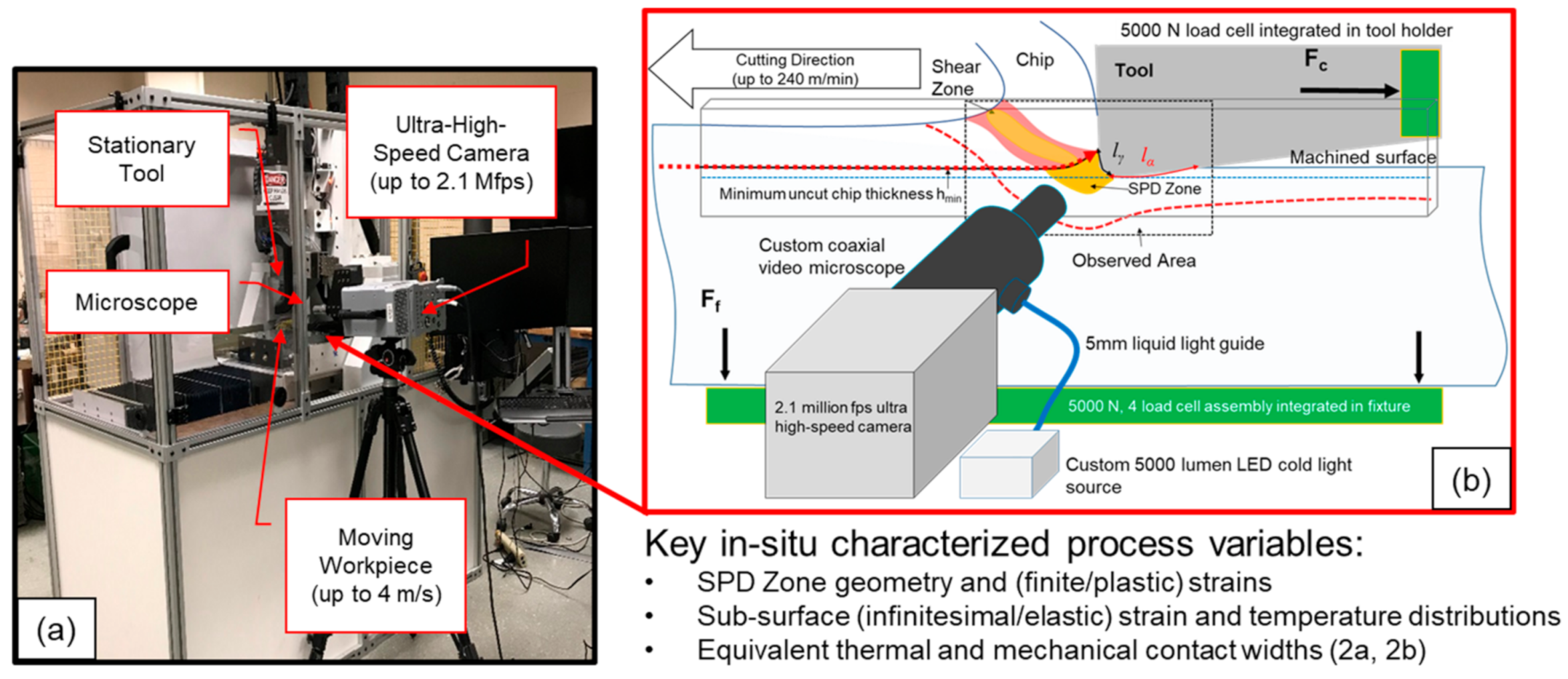
2. Materials and Methods

The proposed analytical methodology is based on efficient experimental characterization of relevant model inputs, most importantly the equivalent Hertzian width of contact (2a), as well as cutting forces and apparent friction coefficient at the minimum chip thickness (hmin) condition. Figure 1 provides and overview of the custom-built in-situ testbed (Figure 1a) and schematically illustrates the kind of orthogonal (2D) plane strain in-situ observation that is carried out on the testbed (Figure 1b). The testbed was constructed on a ~2 ton granite surface plate, with a welded steel base bolted into the building’s concrete foundation, and filled with bags of sand to dampen vibrations. The main cutting stroke (1 m travel length), powered by proprietary linear servo motor by Yaskawa (experimental series SLGFW2, Kitakyushu, Japan) can achieve up to 4 m/s travel speed, with 5 Gs of acceleration and a peak force in excess of 5 kN. Encoder feedback of 50 nm/pulse and travel straightness of better than 5 microns over the entire stroke promote exceptionally smooth speed and positional control. The vertical axis, which controls the uncut chip thickness in 2D cutting (could also be considered depth of cut or feed) features positional repeatability of better than 0.4 microns. Cutting forces are captured by integrated foil strain gauges by Futek (Irvine, CA, USA), which typically achieve better than 0.2 N force measurement accuracy, at a sampling bandwidth of 50 kHz (using Futek’s IAA300 differential amplifier).
The two workpiece materials, AISI 4340 in the annealed condition (18 HRC), and Ti-6Al4V (37 HRC) were evaluated under dry, cryogenic cooling (liquid nitrogen, LN2), and oil-lubrication (UNIST Coolube 2210, proprietary blend of mixed esthers, viscosity of 16 cSt at 40 °C). Cooling and lubrication metalworking fluids were applied from the rake and flank simultaneously. The purpose of selecting these conditions was to evaluate the effect of each cooling and lubricating condition on the tribological behavior of the system, as well as the resulting residual stress. In order to avoid the effect of cutting tool coatings, a new uncoated carbide tool (Kennametal grade K313, NB2R geometry, zero degree rake angle, 5 degree clearance and flank angle, custom ground or polished, cutting edge radius rβ = 15 μm) was used for each trial. All cuts were carried out at a constant cutting speed of 120 m/min (2 m/s) and on a tapered or inclined plane to continuously vary the uncut chip thickness from 0 to approximately 50 μm. The samples were EDM-sectioned and low-stress precision ground and polished to a thickness or width of 3 mm. The sample length (cutting length) was 150 mm, and the height of each sample was approximately 50 mm, although less than a single millimeter was removed during in-situ cutting trials. Both workpiece materials were used in the annealed condition, and were confirmed via XRD analysis to be virtually stress-free in the as-received condition. Sample preparation (e.g., EDM sectioning, grinding, polishing) was conducted in such a manner as to remove the residual surface stress from the previous sample preparation step.
To support model validation, residual stress depth profiles on machined and subsequently electro-polished samples were characterized for the AISI 4340 samples along the cutting direction via X-ray diffraction, using the sin2(ψ) technique on a Rigaku SmartLab diffractometer (Rigaku Americas Corp, Woodlands, TX, USA). For Ti-6Al4V samples, only the surface stress was measured in an effort to highlight the fundamental differences between the response of this high temperature material and the AISI 4340 steel. The room-temperature elastic properties and yield strength for the two workpiece materials are listed in Table 1 below.
While cutting forces and apparent friction coefficients were obtained by determining the onset of chip formation visually, i.e., from high speed in situ images, typically captured at 100,000 frames/second and 159 nanosecond exposure, using a 20× magnification objective (Mitutoyo M Plan APO, Takatsu-ku, Kawasaki, Japan), determination of the equivalent Hertzian (elastic) width of contact (2b) required further post-processing and analysis of the image sequence. Open-source digital image correlation software (ncorr) (Trilion, King of Prussia, PA, USA) was used in Matlab to determine sub-surface strain fields, particularly in the tertiary deformation zone of the workpiece. By locating the exact point of workpiece material springback (i.e., the point at which the workpiece material exist the flank face at a height of hmin above the bottom of the tool tip), and finding the horizontal intersection of this streamline with the beginning of sub-surface plastic deformation in the SPD zone (severe plastic deformation), as illustrated in Figure 2. Likewise, the equivalent contact width in cutting may be determined by finding the shear plane angle, and projecting a right angle line towards the sub-surface ahead of the cut, as shown in Figure 2.

3. Theory and Results

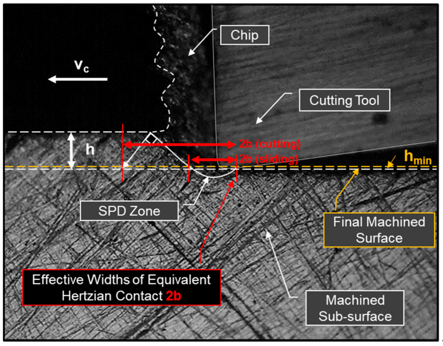
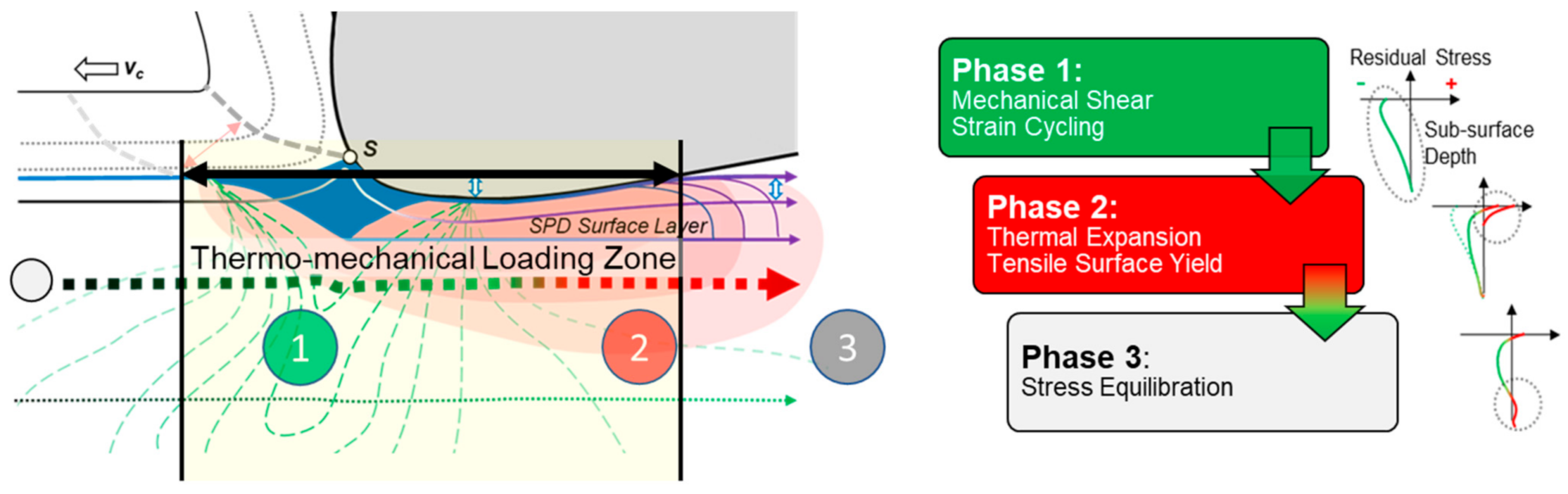
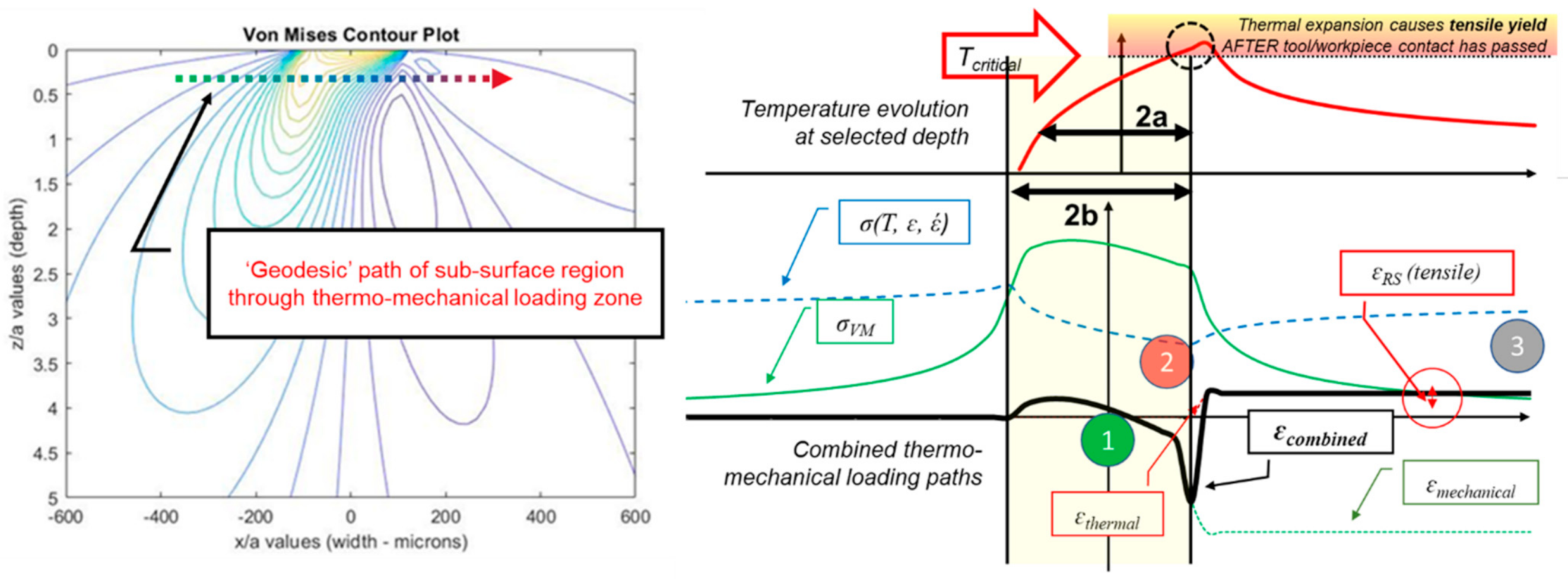
3.1. Thermo-Mechanical Sub-Surface Loading during Machining and Sliding Processes

The author’s multi-domain modeling framework is based on coupled (thermo-mechanical) calculations in the elastic, plastic, thermal, and thermodynamic domains. For more details on the analytical modeling technique, particularly calculations within the thermal domain, which governs thermal softening behavior and near-surface tensile residual stress; interested readers are referred to the author’s previous work [20]. Based on experimental observations and successful modeling efforts, the author hypothesizes that there exists a distinct temporal and causal separation of mechanical and thermal effects in three distinct phases, i.e., Mechanical Stress Formation, due to shear deformation (Phase 1), followed by Thermal Stress Formation, due to thermal expansion (Phase 2) and finally, Stress Equilibration (Phase 3) (see Figure 3). This hypothesis should be considered to be somewhat non-intuitive, due to the interwoven (i.e., generally simultaneous) thermo-mechanical nature of workpiece material elastic and plastic deformation during machining.
The primary reason for the (limited) spatial and temporal separation of mechanical and thermal effects is to the presence (or lack) of the ‘protective’ hydrostatic stress field underneath the sliding and indenting tool edge radius and trailing edge (flank face), where elastic springback due to the minimum chip thickness effect lead to extended tool and workpiece contact. Once the tool has passed, and the workpiece surface is unconstrained, the residually hot surface is free to thermally expand and yield plastically, which occurs relative to the rigid (and relatively cold) sub-surface. This tensile yield only occurs after (generally compressive) stress has already been induced due to mechanical effects, and so the tensile yield due to thermal expansion will be in superposition with prior mechanical residual stresses. Each workpiece material has a characteristic ‘critical temperature’, beyond which tensile stress will be induced as the equivalent stress due to thermal expansion exceeds the yield strength. Therefore, certain cooling and lubricating strategies (e.g., cryogenic machining), or low cutting speeds are expected to yield primarily compressive residual stress fields. Likewise, high-speed, low mechanical load processes, such as grinding, are expected to result in pronounced tensile stress states.

3.2. Thermal Domain Considerations

The highly localized heating and thermal loading on the workpiece surface during tractional sliding is one of the key characteristics of machining and finishing processes. The amount of heat being generated depends primarily on the sliding pair of tool and workpiece material (i.e., the amount of sub-surface plastic work being done, and the surface traction boundary condition), and the resulting temperature profile depends primarily on the thermal properties of the workpiece material. Put another way, sliding generates heat, and this heat input results in temperature rise according to the response of the atoms within the workpiece. The heat source intensity can be modeled as a line heat source of half width a, with intensity proportional to the friction force and sliding speed. For more information on thermal sub-domain modeling, the reader is again referred to the author’s previous work in [20].
Once temperatures are determined from in-situ experimental calibration trials and analytical modeling, the key questions becomes ‘what will the effect of the temperatures be on the workpiece material and tool?’. While this is clearly a complicated question, we will attempt to answer at least the most important aspects of the relative impact of temperature rise (primarily on the tool–workpiece interface on the flank face of the tool) on the workpiece material. To quickly determine material-specific thermal stress response, we propose the use of a stress vs temperature graph, shown for both Ti-6Al4V and AISI 4340 in Figure 4. The graph consists of the workpiece material’s temperature-dependent shear strength (black lines) and the equivalent thermal (expansion) stress, σeq (blue line), which is given by Equation (1). In this equation, α (T) represents the temperature-dependent linear thermal expansion coefficient, ΔT is the difference between the bulk temperature of the workpiece and the peak (flash) temperature induced as a result of tractional sliding, while E(T) and ν(T) are the temperature-dependent functions of Young’s modulus and Poisson’s ratio. It should be noted that the value of the bulk workpiece temperature will depend to some degree on the actual cutting conditions and shape of the near-surface thermal field. In practice, the values of the bulk temperature may be in the range of room temperature (RT, ~20 °C) for low cutting speeds and low thermal numbers, up to ~200 °C in the case of very high cutting speeds and thermal numbers. For most cutting speeds and workpiece materials, a bulk temperature of 100 °C has been found as a reasonable starting point in the author’s recent experimental and modeling efforts.
σ e q = α T E T Δ T 3 1 ν T  
While the workpiece yield strength reduces with temperature (i.e., the workpiece thermally softens), the localized thermal expansion stress becomes more severe. At a material-specific, critical temperature, the stress due to thermal expansion exceeds the workpiece material yield strength, and permanent (plastic) deformation occurs. It should be noted that if this thermal expansion would merely ‘elongate’ the surface layer of the material, no residual stress would result. Rather, it is the very definition of a residual stress to exist as an unrealized or potential strain, which is being constrained due to external boundary conditions, in this case the surrounding base metal of the workpiece. Thus, unrealized plastic strain (potential elongation that cannot be realized as long as boundary conditions are present) is the origin of subsequent tensile residual stress, which is well-known to have detrimental effects on the fatigue life of highly stressed components. Visualizing this stress as a compressed spring, it becomes clear that a positive towards yield has been induced; this is of course not desirable in any circumstance, as the yield strength and hardness will likewise be reduced by this effect, which is sometimes (erroneously, or at the very least misleadingly) referred to as ‘permanent thermal softening’. Once the function of the deviatoric (residual) stress vs temperature (red lines in Figure 4) has been calculated, it is possible to directly convert sub-surface temperature profiles determined via Equation (2) into a resultant, tensile residual stress profile ( σ t R S ).
f   σ e q T i > σ y i e l d T i ,   t h e n   σ t R S T i = σ e q T i    
As can be seen in Figure 4, the critical temperatures and thermally-induced residual stress responses of AISI 4340 and Ti-6Al4V are quite different, with the critical temperature of the alloy steel (~220 °C) being approximately half that of the high-temperature titanium alloy (~480 °C). The yield strength curve for AISI 4340 was obtained from the manufacturer’s ASTM E45-compliant data sheet [21], and the temperature-dependent yield strength data for Ti-6Al4V was extracted from data sheet information reported in [22]. Notably, the slope of thermally-induced residual stress is significantly steeper for the steel workpiece material, which implies that there will be significantly greater sensitivity to any change in sliding temperature due to increased cutting speed and tool wear. Due to its low elastic modulus and limited thermal expansion behavior, Ti-6Al4V exhibits a particularly stable and muted response to localized heating, which comes as no surprise given its typical applications in aerospace and intermediate or high-temperature systems.
It should be noted that critical temperature by itself is only an indicator of a given material’s response to the localized temperature increases, as is the case in sliding, cutting and even additive and welding processes. The actual temperature values, in the case of metal cutting the tool–workpiece interface temperature on the flank face exit point, will depend on the tribological interactions between the tool and workpiece, as well as the rate at which heat is being dissipated (i.e., the relative values of cutting speed, thermal conductivity, heat capacity, and density). For details on how sliding temperatures may be calculated based on in-situ characterized data, the reader is referred to [20], as well as the authors other related works. In all of these efforts, the thermal (Peclet) number of the tool and workpiece sliding pair is one of the most important metrics, and may be calculated according to Equation (3), where vc is the cutting speed in m/s, a is the effective thermal half width of contact in m, and κ (T) represents the temperature-dependent thermal diffusivity of the workpiece material in m2/s. The thermal diffusivity is convenient to use, as it combines a material’s density, heat capacity, and thermal conductivity in a single, combined metric. Like the equivalent elastic and Hertzian width of contact, b, the thermal width of contact, a, may be obtained from in-situ observations of the cutting process, as illustrated qualitatively in Figure 1.
P e = v c   a   2 κ   T  

3.3. Residual Stress Calculation via Elastic Sub-domain Model

Calculations for the elastic sub-domain begin with determining the values for normal and shear stresses along the equivalent mechanical half width of contact of the tool–workpiece interface [23]. These equations represent the case of a cylinder sliding over a plane surface, with the assumption of plane strain conditions for the surface. It should be noted that due to deviations from oversimplifying assumptions of Hertz theory, particularly the condition of non-conformity, it is not possible to derive the half width of contact from this theory. Instead, the proposed approach explicitly relies on in-situ measurement of an equivalent or effective Hertzian contact width (2b), which consists of the tool–workpiece contact region on the flank face, as well as the zone of severe plastic deformation ahead of the cutting edge. Figure 1 illustrates the definition of the equivalent thermal contact width, 2a, which is slightly lower than the 2b due to the limited extent of thermal layer depth δ extending ahead of the primary shear plane, while Figure 5 illustrates how a particle moves through these two zones.
Figure 5 highlights the differences between 2a and 2b, while also providing a comprehensive overview of how the combined thermo-mechanical loading of a specific workpiece sub-surface region occurs when a ‘geodesic’ (relative straight motion) path for this region is traced through the thermal and mechanical fields. It should be noted that accurate determination of the stresses in strains in all three directions (x, y, and z) requires a more comprehensive analytical approach, and cannot be achieved by simply following the path of a particle through the maximum shear stress (e.g., under the Tresca yield criterion).
In order to conduct a closed-form analytical analysis of the sub-surface stress evolution, we shall assume that the sub-surface strain cycle is approximately identical with the perfectly elastic strain cycle, as a calculated from modified tractional Hertz theory described in [20]. Based on this infinitesimal strain assumption, which has been experimentally validated via in-situ observations, it is nevertheless possible to analytically determine incremental (micro-) plastic deformation. While this may appear to be contradictory at first sight, it is merely being proposed that an elastic strain field may be assumed; the stresses, on the other hand, are limited by some flow rule and constitutive relationship. As long as the elastic limit is not exceeded by a large factor (i.e., stresses are to first approximation infinitesimal, even if minor plastic deformation occurs due to strain accumulation), then the elastic strain field will not be distorted.
Following Merwin and Johnson’s [24] approach, the Prandtl–Reuss incremental relations, which are based on small strain deformation theory of an isotropic solid, may be employed to model the stress–strain relationship in the (limited) plastic zone. In these relations, we shall use the stress and strain deviations, which are defined via Equation (4) as the definition of each stress component from the hydrostatic stress and strain components, s and e, respectively.
s = σ x + σ y + σ z 3 ,   s i = σ i s ,   a n d   e = ε x + ε y + ε z 3 ,   e = ε i e  
For plain strain deformation in the xy plane, the von Mises flow rule in terms of the stress deviations, as is commonly used in the case of ductile metals, is defined as keeping the second invariant of the stress deviation tensor J2 constant and equal to k2, as shown in Equation (5).
J 2 = 1 2 s x + s y + s z 2 + τ x y   2 = k 2
In the previously quoted Prandtl–Reuss relations, the rate at which stresses do work as a change in shape occurs (W) can be written as shown in Equation (6). As tractional sliding occurs in a single direction (in our case the x direction), the rate of change for each strain deviation can be taken relative to this direction. In this scheme, W(dot) can be interpreted as the rate at which energy is irreversibly dissipated through plastic deformation, and thus needs to always be larger than zero, or deformations will be elastic, and thus simply be governed by Hooke’s Law.
W ˙ = s x e x x + s y e y x + s z e z x + τ x y   γ x y x  
The Prandtl–Reuss relations may now be stated by relating the change in stress deviation during tractional sliding in the x direction, as shown in Equation (7), where G represents the elastic shear modulus.
s i x = 2 G e i x + W ˙ 2 k 2 s i  
A full analysis at each incremental sub-surface depth y can now be performed to determine the evolution of stress and strain deviation for a known elastic stress field. Such an analysis follows each stress and strain component along the entire path of elastic and plastic sub-surface deformation due to the boundary condition applied at the surface (i.e., the sliding cutting or burnishing tool, with their characteristic normal pressure and equivalent contact width). As there can be no residual traction after the tool has passed, it is necessary to apply the conditions of equilibrium for a plane (smooth or ripple-free) surface free from traction. As a result of the conditions imposed by plane strain deformation, there can only be two residual stress components in plane strain deformation (i.e., in the x and z directions), both of which are a function of depth (y) only (see Equation 8). Therefore, we can write:
σ x R S = f y ,   σ z R S = f y ,   w h i l e     σ y R S = τ x y   R S = τ y z   R S = τ z x   R S = 0  
As a result of Equation (8), the incrementally calculated residual stress components σ i r as x are required to relax and interact with one another to yield a proper equilibrium. Specifically, the (forbidden) quasi-residual stress component in the depth (y) direction σ y r is subtracted in a ratio according to the Poisson’s ratio ν. Notably, the difference between the x and z sub-surface residual stresses is typically limited to relatively minor deviations in the shape of the residual stress field, i.e., the sub-surface peak magnitude and location are similar, as well as the total affected layer depth, typically between 2–3 b, while the (near-) surface residual stress in the out-of-plane (z) direction tends to be more compressive (and thus the ‘best case’ with respect to fatigue life and repeated or shakedown loading). Consequently, initial examination of the residual stress in the cutting and tangential (x) direction can often be used as a reasonable first approximation of the ‘overall’ state of residual stress in the sub-surface.
σ x R S = f y = σ x r ν σ y r 1 ν ,   a n d   σ z R S = f y = σ z r ν σ y r 1 ν  
While strains and strain rates in the primary (shear) deformation zone during metal cutting may exceed 500% and 105, respectively, the regime of sub-surface deformation giving rise to mechanically-induced residual stresses is far less extreme. Of course, the extreme conditions at the top machined surface in the severe plastic deformation (SPD) zone do require highly sophisticated material models. However, the proposed approach experimentally measures this highly complicated approach as the equivalent elastic width of contact (2b) and SPD depth are determined via in-situ observations. Thus, the simple Johnson and Cook’s (JC) phenomenological constitutive model (or any similar constitutive relationships) may be used to capture the effects of thermal softening, strain rate, and strain hardening in the workpiece sub-surface below the SPD zone (see Equation 10) [25]. Model parameters can typically be obtained through literature, and further (inversely) calibrated and validated from in-situ digital image correlation (DIC) data. It should be noted that the ‘simple’ form of the JC model provided by Equation (10) is generally not suitable for large deformations at elevated temperatures, which may lead to dynamic recrystallization (DRX) or other flow softening mechanisms. As residual stress formation occurs primarily due to infinitesimal (quasi-elastic) strain accumulation below the zone of severe plastic deformation, the standard (non-modified) form of the JC model can be considered very much appropriate for sub-surface residual stress prediction and modeling, assuming of course that the effects of the primary (shear plane) and tertiary (SPD) deformation zones are well-known, as is the case in the current paradigm by means of experimental in-situ characterization.
σ = A + B ε p n 1 + C ε p ˙ ε ˙ 0 1 T T 0 T m T 0 m  

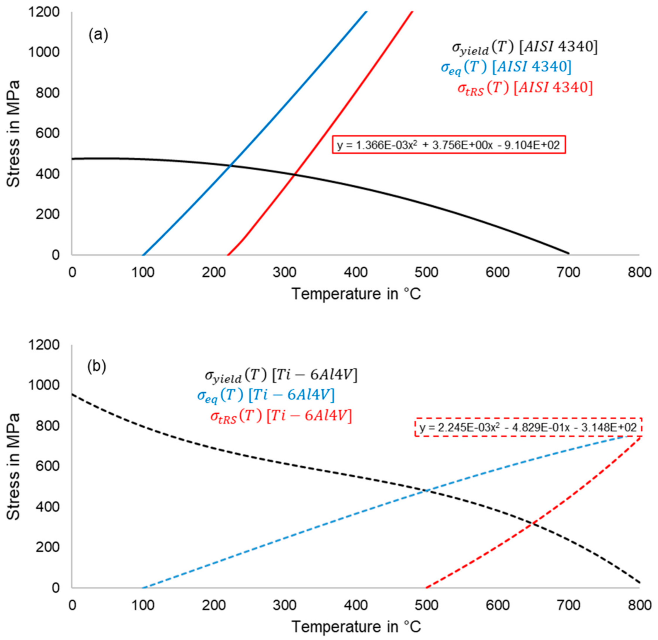
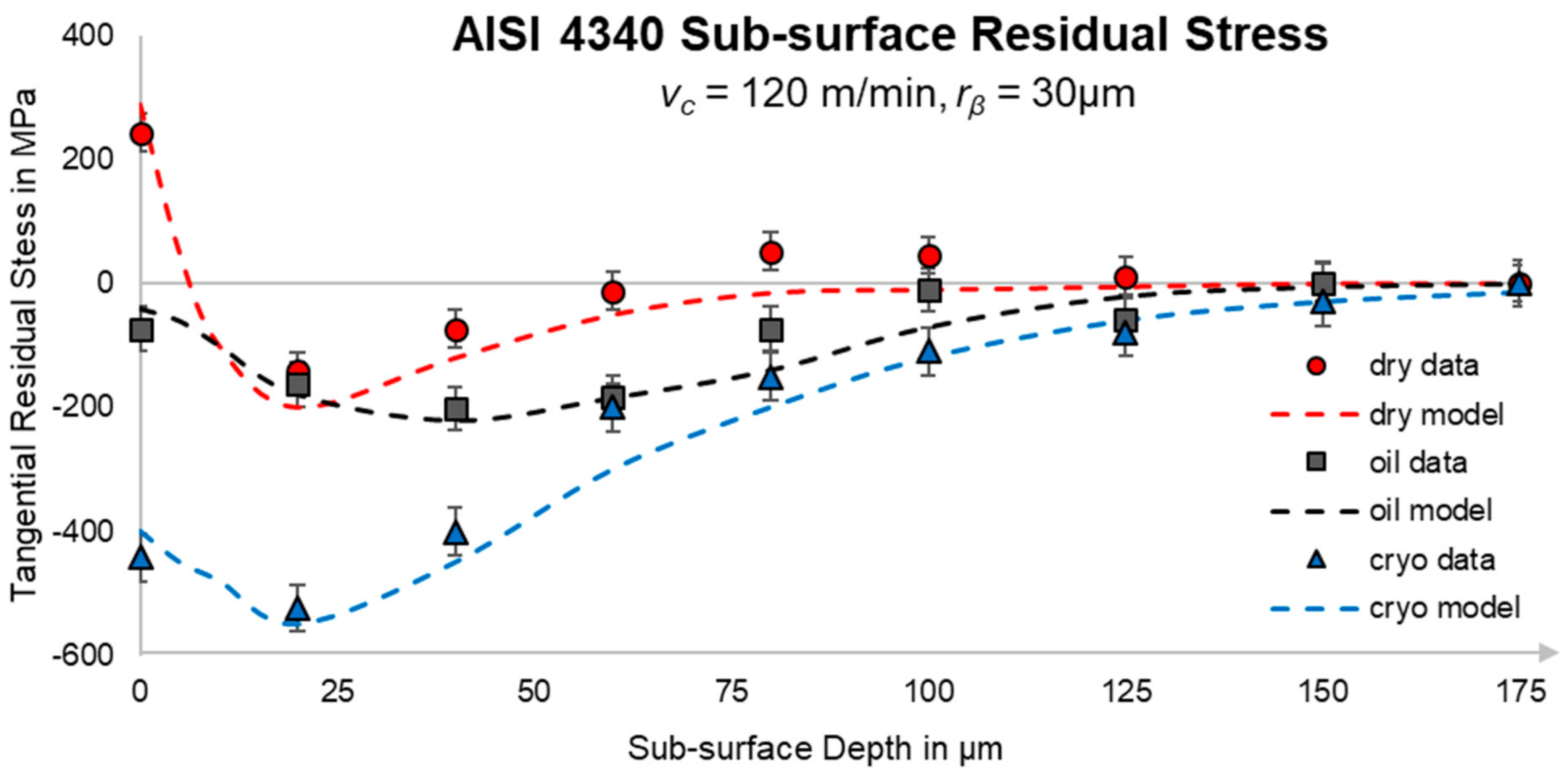
3.4. Preliminary Calibration and Validation of Proposed Model in AISI 4340

Following in-situ experimental trials to calibrate key model input parameters, validation of the proposed residual stress model was been carried out in alloy steel AISI 4340. Comparisons of model-predicted sub-surface residual stress in the tangential (cutting) direction and XRD-validated data are shown in Figure 6. The constitutive material response of steel and titanium workpiece materials is quite different, and thus these materials were selected to evaluate the ability of the proposed model to capture material-specific response to the complex thermo-mechanical loading of machining. In addition to the effects of cutting speed, tool edge hone and radius and tool-wear (currently limited to flank wear), the model also captures the effects of depth of cut and feed by considering the influence these process parameters have on the morphology and intensity of the shear zone in the area of surface generation (see Figure 1). The forces, and apparent friction coefficient obtained from in-situ analysis at the onset of chip formation, or sliding and ploughing, as shown in Figure 2, i.e., h = hmin, as well as the effective elastic contact 2b width at an uncut chip thickness of 30 μm, are listed in Table 2 below.

4. Discussion

4.1. Limitations and Future Expansion Needs of Proposed Model

Due to the focus on surface integrity, the model discussed in this paper does not take into account details of chip formation, including the energy of new surface generation and strain at fracture. During segmented chip formation, this may significantly impact the predictive power of the model, which assumes a quasi-steady-state (i.e., continuous chip formation). Moreover, the model currently only considers finish machining conditions, i.e., low feed and depth of cut scenarios. For large values of uncut chip thickness, the effect of the large shear plane on sub-surface stress asymmetry is expected to become significant enough to cause major deviations. Ongoing in-situ studies are being conducted to better study and accurately capture these physical effects within the proposed modeling paradigm. Finally, the plane-strain assumptions made by the proposed model are clearly not representative of the complex (three-dimensional) state of stress of geometrically complex machining operations, such as milling processes. While a comprehensive discussion of this final point lies outside of the scope of the present work, the author has been able to implement the present modeling approach for complex milling, drilling, and turning operations. This is achieved by dividing the complex sickle-shaped geometry of the uncut chip into infinitesimal slices of width ∂h.
Outside of the very beginning and end of the uncut chip, each of these slices can be approximated as a single plane-strain (technically oblique) cut. By integrating the relative contribution of each of these 2D slices back onto the 3D reference coordinate system (e.g., the free-form workpiece surface being milled), it is possible to obtain a reasonable approximation of the actual residual stress profile, including the residual shear strain. It should be noted that the boundary and relaxation conditions in three-dimensional cutting are less restrictive than they are in plane strain (orthogonal cutting). Thus, it is not possible to directly compare a given 2D residual stress prediction and apply it directly to a 3D cut. Nevertheless, the author’s research group’s ongoing and future work are focused on determining the most efficient manner of achieving reliable and robust residual stress predictions in 3D machining operations.

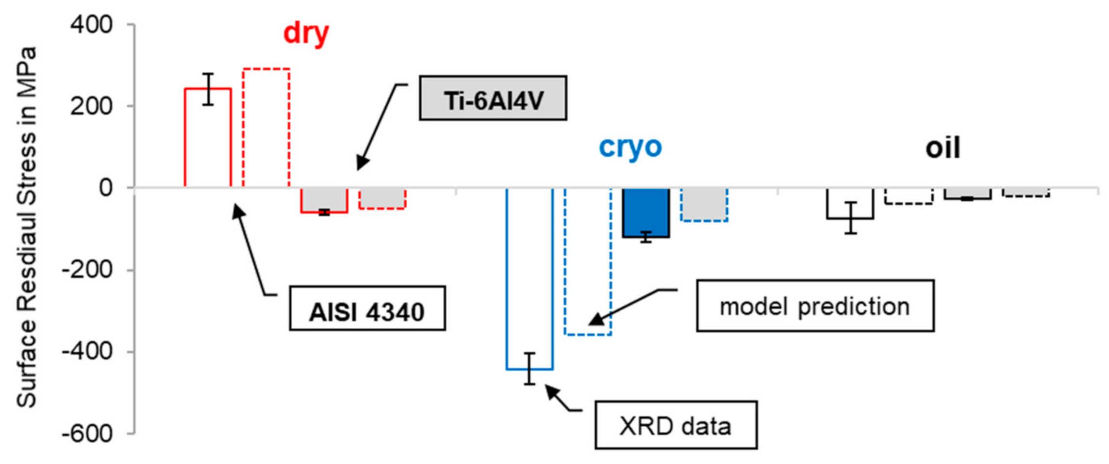
4.2. Comparison and Interpretation of Experimental Data and Model Predictions

The data shown in Figure 6 and Figure 7 are based on calculations and equations laid out in Section 3. Specifically, the thermo-mechanical loading of each sub-surface depth is carried out as illustrated in Figure 3 and Figure 5, using the equations laid out in Section 3.3. As can be seen in Figure 6, the correlation between experimental and modelled residual stress profiles is well within an acceptable 20% deviation, and indeed within the experimental scatter of the XRD experimental data. Thus, it appears that the qualitative (and quantitative) effects of cutting speed and cooling and lubricating condition are effectively captured by the proposed model. Modeling of cryogenic cooling (LN2 flow rate of 50 mL/min, directed at the flank and rake faces) was carried out by using the in-situ characterized contact widths and forces shown in Table 1, and simply reducing the maximum (flash) temperature (in the thermal domain sub-model) by the temperature of liquid nitrogen, i.e., −195.8 °C. While this ‘temperature superposition’ approach is clearly overly simplistic and neglects kinetic effects, such as Leidenfrost boiling, it effectively suppresses the inclusion of thermally-induced tensile stresses, leaving only mechanical stress contributions in the final predicted profiles.
Since the measured data (and indeed, the findings of various investigators in the literature) appear to reflect this reality, the results are presented as an example of the potential of using simplifying heuristics to promote real-time modeling, e.g., in industry. The author hypothesizes that the ability to in-situ characterize contact widths and forces does allow for significant simplification of the overall modeling framework, since the key boundary conditions are well known (unlike in more complex numerical frameworks). Once calibrated, the proposed model outputs these results in real-time, i.e., within milliseconds. This computational efficiency, which is gained as a direct result of the high-quality in-situ input data, allows for rapid iteration of countless ‘what if’ scenarios, allowing for rapid optimization of machining parameters for optimum surface integrity.
The sub-surface residual stress data shown in Figure 6 for AISI 4340 alloy steel show that there is a significant difference between the various cooling and lubrication conditions under investigation. While insufficient conditions and data were obtained to make broad conclusions about the effects of coolants and lubricants in general, the limited data obtained for the uncoated carbide tool at a speed of 120 m/min do appear to support some qualitative insights into the effect of either cooling and lubrication on the residual stress profiles that were modeled and subsequently measured and validated. Most notably, dry cutting lead to (limited) tensile surface stress, which occurred due to heating beyond the critical temperature of AISI 4340 shown in Figure 4a. The depth and magnitude of this thermally-induced tensile surface stress were limited at the 120 m/min cutting speed, but would be expected to increase significantly at higher speeds, or with increasing tool-wear.
Lubrication resulted in slightly reduced normal force and significantly decrease sliding and friction force at h = hmin, i.e., reduced friction when compared to dry cutting (0.52 vs 0.13 apparent friction coefficients for dry and lubricated cutting, respectively). Due to the reduced friction force, less heat is being generated during oil-lubricated machining. Therefore, the surface temperature was sufficiently reduced to eliminate any thermally-induced tensile surface stress at this cutting speed. Moreover, affected depth of the lubricated cut was increased over that of the dry cut, which is in line with similar observations in burnishing process, and indeed, follows from the predictions of modified Hertz theory [23].
Cryogenically-cooled machining (liquid nitrogen as a coolant, no lubrication) resulted in the most compressive surface and sub-surface peak residual stresses, as well as the largest affected layer depth. This experimental finding is consistent with those by several other researchers in multiple other workpiece materials (e.g., see [15]). Our in-situ characterization efforts suggest that cryogenic cutting significantly increases both the contact width and normal force, while slightly reducing the friction when compared to the dry condition. In other words, cryogenic cooling increases the ‘rigidity’ of the workpiece response to the sliding cutting tool, which would in fact be the expected result of increased workpiece yield strength at lower temperatures. Moreover, contact widths increase, resulting in significantly increased affected layer depths of compressive residual stress (and likely significant sub-surface strain hardening). This may be desirable in some applications, e.g., bearing races and critical, highly stressed features on turbine blade that do not require large amounts of ductility, but rather high hardness and compressive residual stress (RS).
By increasing the depth and magnitude of compressive residual stresses, cryogenic cooling does not merely ‘quench’ and cool the cut the eliminate the negative effects of the heat generated during dry cutting, but a positive benefit in terms of increased compressive stresses is gained. However, the increased cutting forces that go along with this increased mechanical strengthening of the cryogenically machined surface may not be acceptable in some applications, such as thin-walled turbine blades and long and slender shafts. Therefore, future work will need to investigate the trade-off and optimization of the positive effects of cooling with those of lubrication, as has been preliminarily done in some of the author’s previous work for ‘hybrid’ high speed cryogenic machining of Ti-6Al4V with polycrystalline diamond tools (PCD) [26]. In that particularly study, reduced cutting forces and increased tool-life were noted for the combined cryogenic and oil lubrication mode, which was compared to cryogenic-only and oil lubricated machining.
In some cases, reducing the degree to which the sub surface is affected may also be desirable, particularly when a component’s design depends primarily on the assumption that the bulk and virgin properties of the base metal are maintained at or near the machined surface. Therefore, a tailored component-specific approach is necessary to conduct ‘pro-active surface engineering’. The present manuscript proposes an integrated methodology of rapid in-situ characterization to calibrate semi-analytical process models acting in real-time, which could be a significant enabler for this future capability in industry.
As a result of the higher critical temperature of Ti-6Al4V (see Figure 4b), even dry cutting under the trial conditions did not result in a surface tensile stress. However, the titanium workpiece material also exhibited a less pronounced response to cryogenic cutting, with less than half the compressive surface residual stress than that measured and modeled for AISI 4340. Overall, model results were well-within experimental error margins, and the qualitative behavior of the two workpiece materials and the three modes of cooling and lubrication was captured with excellent fidelity.
Figure 7 provides additional results comparing the magnitude of the surface residual stress for AISI 4340 alloy steel and Ti-6Al4V titanium alloy. As can be seen, only the alloy steel exhibited any kind of tensile surface stress under the dry condition, at the relatively limited cutting speed and with an unworn cutting tool of 15 μm cutting edge radius. All other surface residual stress measurements revealed compressive states, although the lubricated condition resulted in the lowest overall surface stress. This observation suggests that reduced friction at the tool–workpiece interface (particularly on the flank face) effectively suppresses both tensile and compressive stress formation, and the surface is left in a more ‘virgin’ condition when compared to other modes of cooling and lubrication. Indeed, this would further support the widespread use of neat cutting oils in the aerospace and automotive industry, particularly when machining high-value and thermally sensitive components.

5. Conclusions

A novel predictive semi-analytical modeling framework for real-time prediction of residual stress has been developed and preliminarily validated in AISI 4340 alloy steel and Ti-6Al4V. Inputs for the semi-analytical process model were acquired through a novel high-speed in-situ characterization technique.
Some key findings include:
  • The critical temperature of a workpiece material, beyond which localized thermal expansion of the surface results in a thermally-induced tensile residual stress, varies significantly between workpiece materials, and is a key metric in residual stress response to cutting.
  • Dry cutting leads to the highest cutting temperatures and most shallow and tensile residual stress profile.
  • Oil lubrication reduces near-surface residual stresses, and generally provides and deeper and more compressive residual stress profile than dry cutting.
  • Cryogenic cooling significantly increases normal force and contact width, which results in a significantly more compressive and deeper residual stress profile.
  • The proposed semi-analytical model was able to capture all of these effects by means of efficient in-situ calibration, and following a qualitatively accurate (physics-based) analytical formulation.
Implementation of real-time residual stress modeling is expected to significantly improve advanced manufacturers’ ability to conduct reliable and results-oriented process modeling, e.g., through the construction of Digital Twins for aerospace finish machining processes. Integration of real-time process-induced stress prediction is also envisioned to aid during the development of next-generation materials, by allowing for early identification of potential manufacturing-stage issues (e.g., excessive strain hardening and propensities to develop tensile residual stress). Future and ongoing work will focus on expanding the set of pedigreed validation data across a broad range of material systems and more complex (three-dimensional) machining operations, such as milling and drilling.

Funding

This material is based upon work supported by the U.S. Department of Energy’s Office of Energy Efficiency and Renewable Energy (EERE) under the Advanced Manufacturing Office’s (AMO) DE-FOA-0001980, Award Number DE-EE0009121/0000, project title “AI-Enabled Discovery and Physics Based Optimization of Energy Efficient Processing Strategies for Advanced Turbine Alloys”.

Institutional Review Board Statement

Not applicable.

Informed Consent Statement

Not applicable.

Data Availability Statement

The preliminary data presented in this study are available on request from the corresponding author, and will be posted on the author’s institutional research website at https://www.engr.uky.edu/ism/research/amse (accessed on 2 March 2021).

Acknowledgments

The author would like to acknowledge support in obtaining XRD residual stress data by Xiyu Wen at Secat Inc. in Lexington, KY, USA.

Conflicts of Interest

The author declares no conflict of interest.

References

  1. Henriksen, E.K. Residual Stresses in Machined Surfaces; ASME: New York, NY, USA, 1948. [Google Scholar]
  2. Halverstadt, R. Analysis of residual stress in ground surfaces of high-temperature alloys. Trans. Am. Soc. Mech. Eng. 1958, 80, 80–85. [Google Scholar]
  3. Kahles, J.; Field, M. Paper 4: Surface Integrity—A New Requirement for Surfaces Generated by Material-Removal Methods. In Proceedings of the Institution of Mechanical Engineers, 1 June 1967; SAGE Publications Sage: London, UK, 1967; Volume 182, pp. 31–45. [Google Scholar]
  4. Barash, M.; Schoech, W. Semi-Analytical Model of the Residual Stress Zone in Orthogonal Machining. In Advances in Machine Tool Design and Research, Proceedings of the Internat. M. T. D. R. Conference, Manchester, UK, 15-17 September 1971; Pergamon Press: Oxford, UK, 1971; pp. 603–613. [Google Scholar]
  5. Pomeroy, R.J.; Johnson, K.L. Residual stresses in rolling contact. J. Strain Anal. 1969, 4, 208–218. [Google Scholar] [CrossRef]
  6. Liu, C.R.; Barash, M.M. The Mechanical State of the Sublayer of a Surface Generated by Chip-Removal Process—Part 1: Cutting With a Sharp Tool. J. Eng. Ind. 1976, 98, 1192–1199. [Google Scholar] [CrossRef]
  7. Liu, C.R.; Barash, M.M. The Mechanical State of the Sublayer of a Surface Generated by Chip-Removal Process—Part 2: Cutting With a Tool With Flank Wear. J. Eng. Ind. 1976, 98, 1202–1208. [Google Scholar] [CrossRef]
  8. Jacobus, K.; Devor, R.E.; Kapoor, S.G. Machining-Induced Residual Stress: Experimentation and Modeling. J. Manuf. Sci. Eng. 1999, 122, 20–31. [Google Scholar] [CrossRef]
  9. Fergani, O.; Lazoglu, I.; Mkaddem, A.; El Mansori, M.; Liang, S.Y. Analytical modeling of residual stress and the induced deflection of a milled thin plate. Int. J. Adv. Manuf. Technol. 2014, 75, 455–463. [Google Scholar] [CrossRef]
  10. Pan, Z.; Feng, Y.; Ji, X.; Liang, S.Y. Turning induced residual stress prediction of AISI 4130 considering dynamic recrystallization. Mach. Sci. Technol. 2017, 22, 507–521. [Google Scholar] [CrossRef]
  11. Shan, C.; Zhang, M.; Zhang, S.; Dang, J. Prediction of machining-induced residual stress in orthogonal cutting of Ti6Al4V. Int. J. Adv. Manuf. Technol. 2020, 107, 2375–2385. [Google Scholar] [CrossRef]
  12. Wang, S.; Li, J.; He, C.; Xie, Z. A 3D analytical model for residual stress in flank milling process. Int. J. Adv. Manuf. Technol. 2019, 104, 3545–3565. [Google Scholar] [CrossRef]
  13. Zhou, R.; Yang, W. Analytical modeling of machining-induced residual stresses in milling of complex surface. Int. J. Adv. Manuf. Technol. 2019, 105, 565–577. [Google Scholar] [CrossRef]
  14. Li, B.; Deng, H.; Hui, D.; Hu, Z.; Zhang, W. A semi-analytical model for predicting the machining deformation of thin-walled parts considering machining-induced and blank initial residual stress. Int. J. Adv. Manuf. Technol. 2020, 110, 139–161. [Google Scholar] [CrossRef]
  15. Jawahir, I.; Brinksmeier, E.; M’Saoubi, R.; Aspinwall, D.; Outeiro, J.; Meyer, D.; Umbrello, D.; Jayal, A. Surface integrity in material removal processes: Recent advances. CIRP Ann. 2011, 60, 603–626. [Google Scholar] [CrossRef]
  16. Arrazola, P.; Özel, T.; Umbrello, D.; Davies, M.; Jawahir, I. Recent advances in modelling of metal machining processes. CIRP Ann. 2013, 62, 695–718. [Google Scholar] [CrossRef]
  17. Umbrello, D.; M’Saoubi, R.; Outeiro, J. The influence of Johnson–Cook material constants on finite element simulation of machining of AISI 316L steel. Int. J. Mach. Tools Manuf. 2007, 47, 462–470. [Google Scholar] [CrossRef]
  18. Kaynak, Y.; Manchiraju, S.; Jawahir, I.S. Modeling and Simulation of Machining-Induced Surface Integrity Characteristics of NiTi Alloy. Procedia CIRP 2015, 31, 557–562. [Google Scholar] [CrossRef] [Green Version]
  19. Liu, X.; Devor, R.E.; Kapoor, S.G. An Analytical Model for the Prediction of Minimum Chip Thickness in Micromachining. J. Manuf. Sci. Eng. 2006, 128, 474–481. [Google Scholar] [CrossRef]
  20. Schoop, J.; Adeniji, D.; Brown, I. Computationally efficient, multi-domain hybrid modeling of surface integrity in machining and related thermomechanical finishing processes. Procedia CIRP 2019, 82, 356–361. [Google Scholar] [CrossRef]
  21. Lescalloy® 4340 VAC-ARC® Data Sheet; Latroboe Speciality Steel Company: Latrobe, PA, USA, 2007.
  22. Ti-6Al-4V Data Sheet; Report TMC-0150; TIMETAL; Titanium Metals Corporation: Henderson, NV, USA, 2000.
  23. McEwen, E. Stresses in Elastic Cylinders in Contact Along a Generatix. Philos. Mag. 1949, 40, 454–460. [Google Scholar]
  24. Applied Mechanics Group; Merwin, J.E.; Johnson, K.L. An Analysis of Plastic Deformation in Rolling Contact. Proc. Inst. Mech. Eng. 1963, 177, 676–690. [Google Scholar] [CrossRef]
  25. Melkote, S.N.; Grzesik, W.; Outeiro, J.; Rech, J.; Schulze, V.; Attia, H.; Arrazola, P.-J.; M’Saoubi, R.; Saldana, C. Advances in material and friction data for modelling of metal machining. CIRP Ann. 2017, 66, 731–754. [Google Scholar] [CrossRef] [Green Version]
  26. Schoop, J.; Sales, W.F.; Jawahir, I.S. High Speed Cryogenic Finish Machining of Ti-6Al4V with polycrystalline diamond tools. J. Mater. Process. Technol. 2017, 250, 1–8. [Google Scholar] [CrossRef]
Figure 1. The author’s recently developed in-situ testbed (a) and associated methodology for integrated characterization and modeling machining and finishing processes (b). Note: SPD = severe plastic deformation.
Lubricants 09 00028 g001
Figure 2. Illustration of in-situ high-speed image of dry cutting condition, with relevant metrics and zones highlighted. In practice, the equivalent width of contact 2a is most accurately determined with help of digital image correlation (DIC) software. [10× objective magnification, 159 nanosecond exposure, vc = 120 m/min, h = 70 μm].
Lubricants 09 00028 g002
Figure 3. Schematic Representation of the Three Proposed Phases of Residual Stress Formation during Machining and Burnishing, based on the approach laid out in [20].
Lubricants 09 00028 g003
Figure 4. Critical temperature graphs for approximating residual stress due to localized heating of AISI 4340 (a) and Ti-6Al4V (b).
Lubricants 09 00028 g004
Figure 5. Schematic overview of modelled thermo-mechanical evolution of stress and strain during tractive sliding in machining. Note: cutting edge is located between the vertical axis intersection (a or b = 0) and the trailing edge contact (a or b = 1).
Lubricants 09 00028 g005
Figure 6. Modeled (dashed lines) and XRD-validated machining-induced residual stress profiles in machining of AISI 4340 alloy steel [vc = 120 m/min, rβ = 15 μm, h =30 μm].
Lubricants 09 00028 g006
Figure 7. Comparison between measured (solid lines) and modeled (dashed lines) surface residual stress for AISI 4340 (white fill) and Ti-6Al4V (gray fill) [vc = 120 m/min, rβ = 15 μm, h =30 μm].
Lubricants 09 00028 g007
Table 1. Elastic properties and tensile yield strength for Ti-6Al4V and AISI 4340.
Workpiece MaterialE (20°C) [GPa]G (20°C) [GPa]νσyield (20 °C) [MPa]
AISI 4340206800.28475
Ti-6Al4V113430.331015
Table 2. Overview of in-situ characterized model input (calibration) data for Ti-6Al4V and AISI 4340.
Workpiece MaterialCooling/Lubricating Condition2b [μm]
(h = 30 μm)
2b [μm]
(h = hmin)
Fc [N]
(h = hmin)
Ff [N]
(h = hmin)
μapparent
(h = hmin)
AISI 4340Dry452636690.52
AISI 4340Cryogenic Cooling (LN2)5835381010.38
AISI 4340Lubrication48298610.13
Ti-6Al4VDry362128520.40
Ti-6Al4VCryogenic Cooling (LN2)462720620.32
Ti-6Al4VLubrication392316510.31
Publisher’s Note: MDPI stays neutral with regard to jurisdictional claims in published maps and institutional affiliations.

