Simulation Analysis of Erosion–Corrosion Behaviors of Elbow under Gas-Solid Two-Phase Flow Conditions


Abstract
1. Introduction
2. Simulation Model
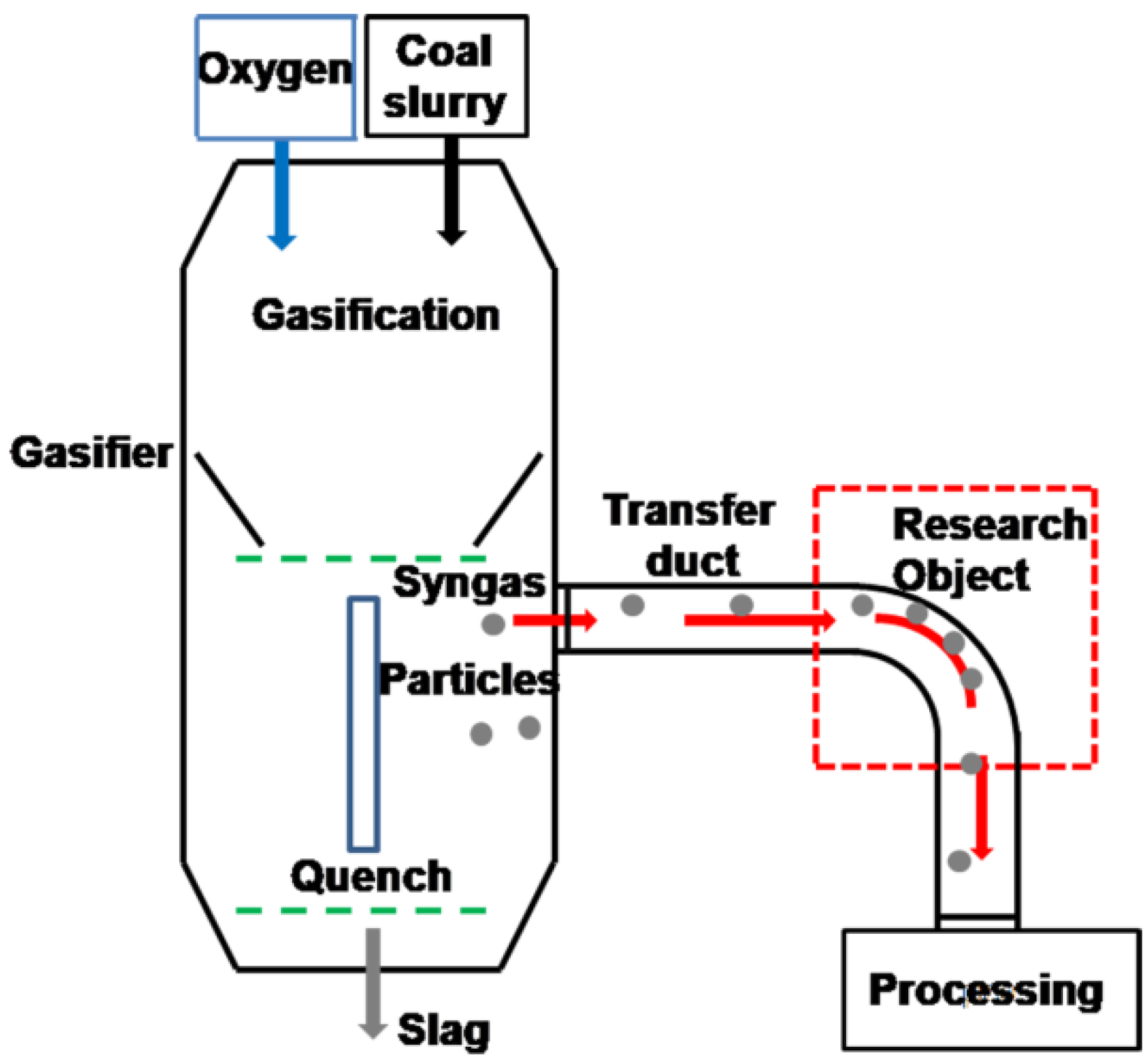
2.1. Simplification of Chemical Equipment
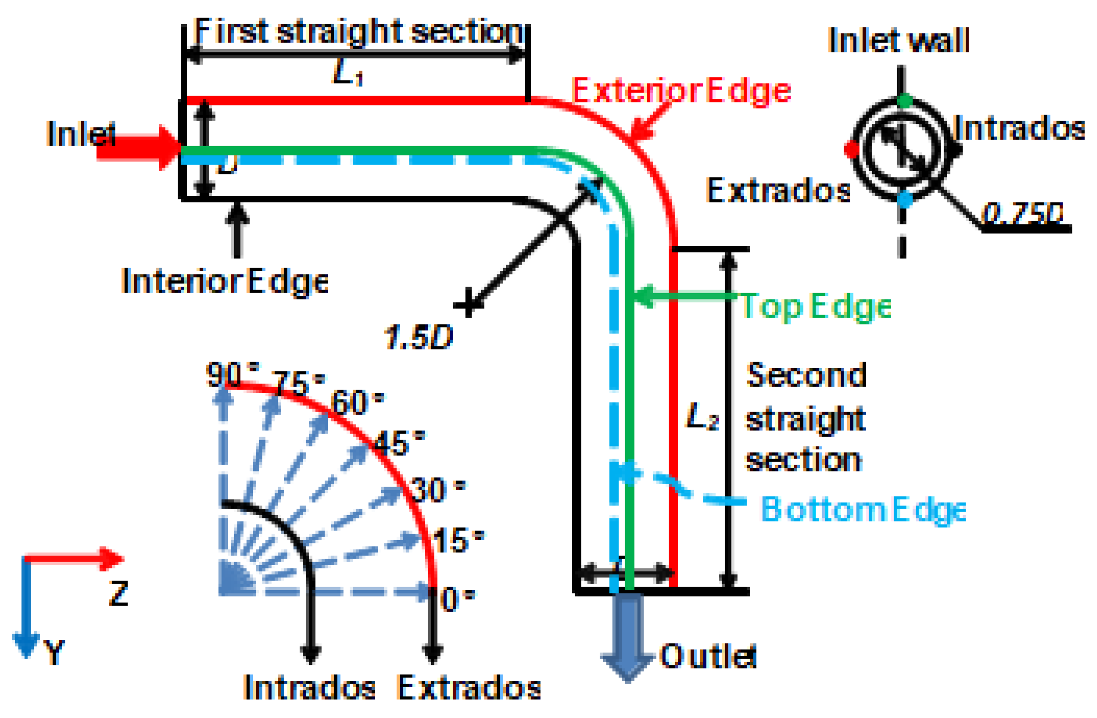
2.2. Geometry
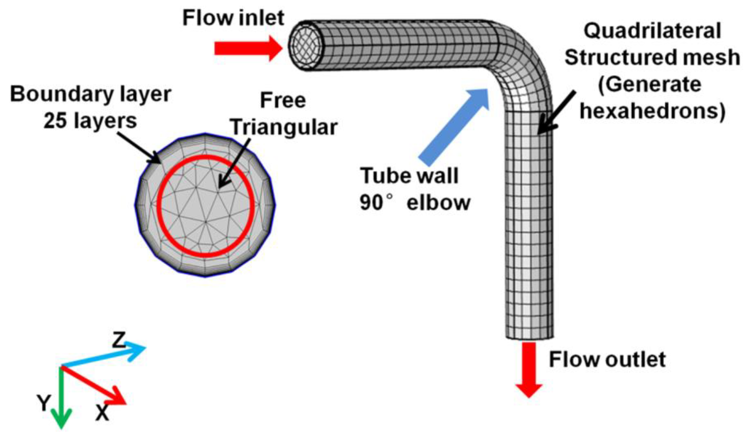
2.3. Mesh
2.4. The Mathematical Simulation Model
2.4.1. Turbulence
2.4.2. Erosion
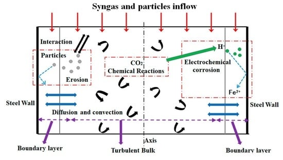
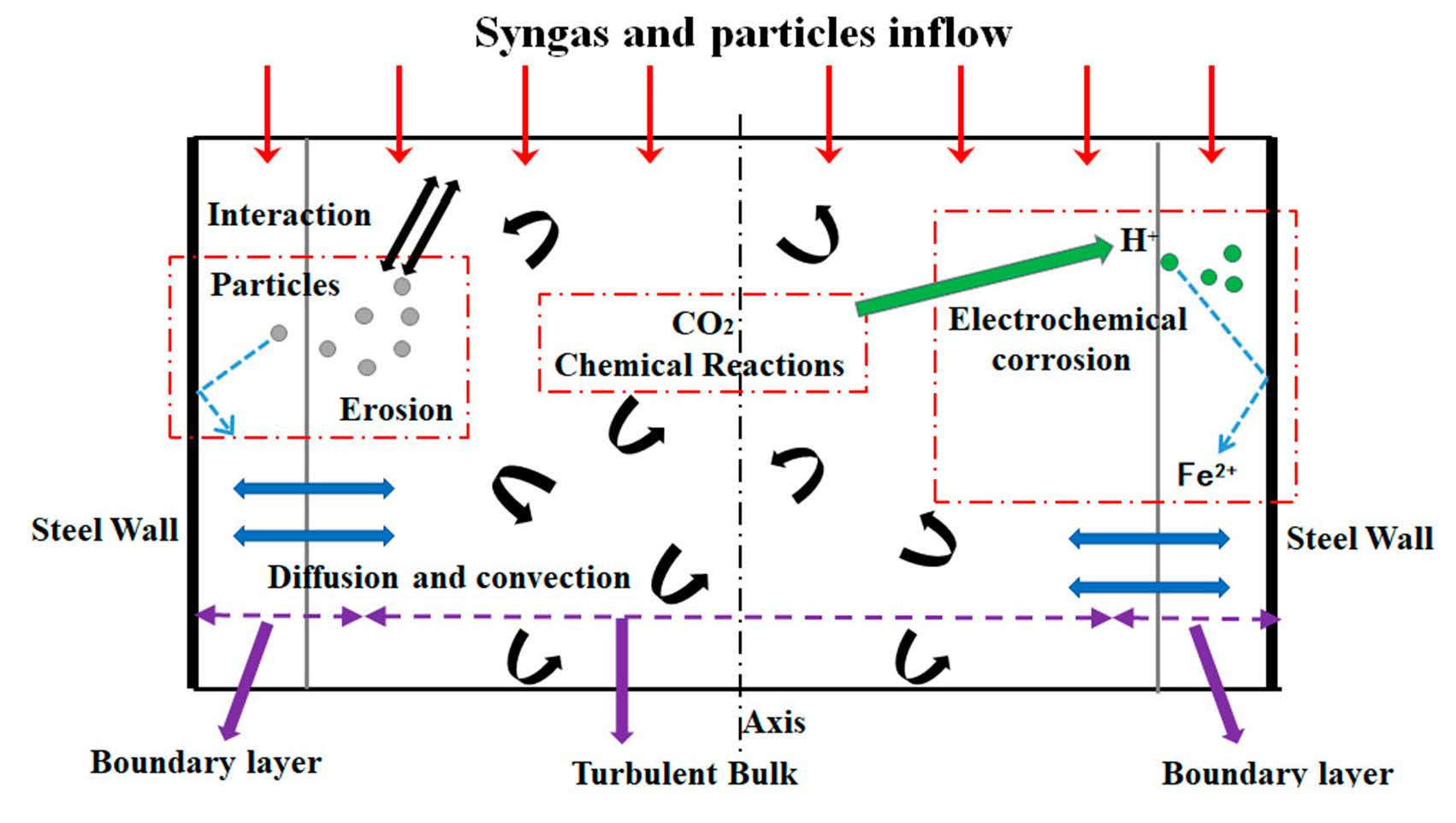
2.4.3. Chemical Reaction and Electrochemical Corrosion
3. Results
3.1. Turbulence Characteristics of Gas
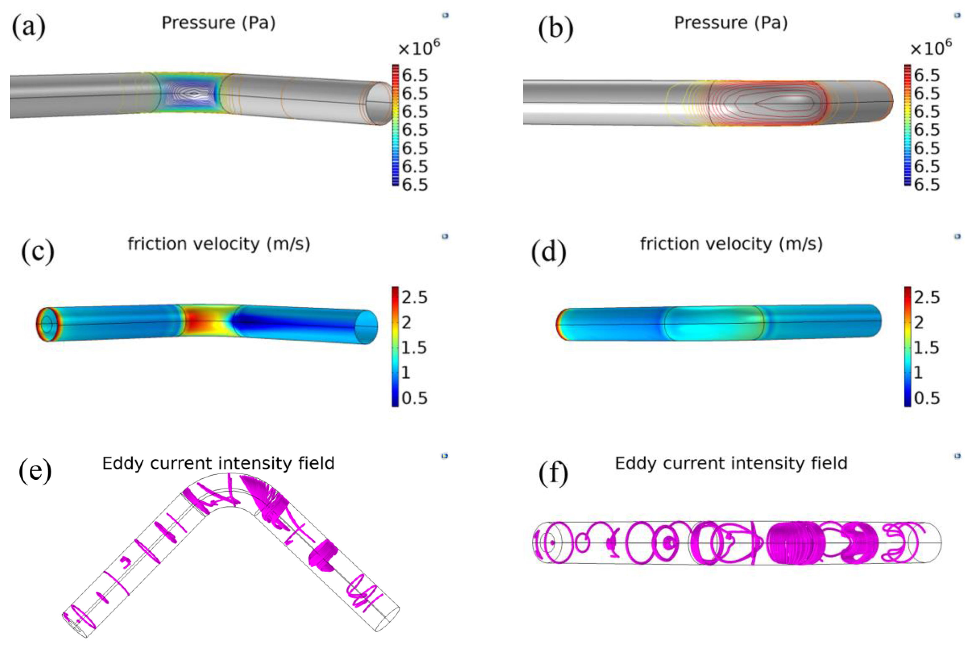
3.1.1. Pressure, Friction Speed Characteristics, and Turbulence Intensity
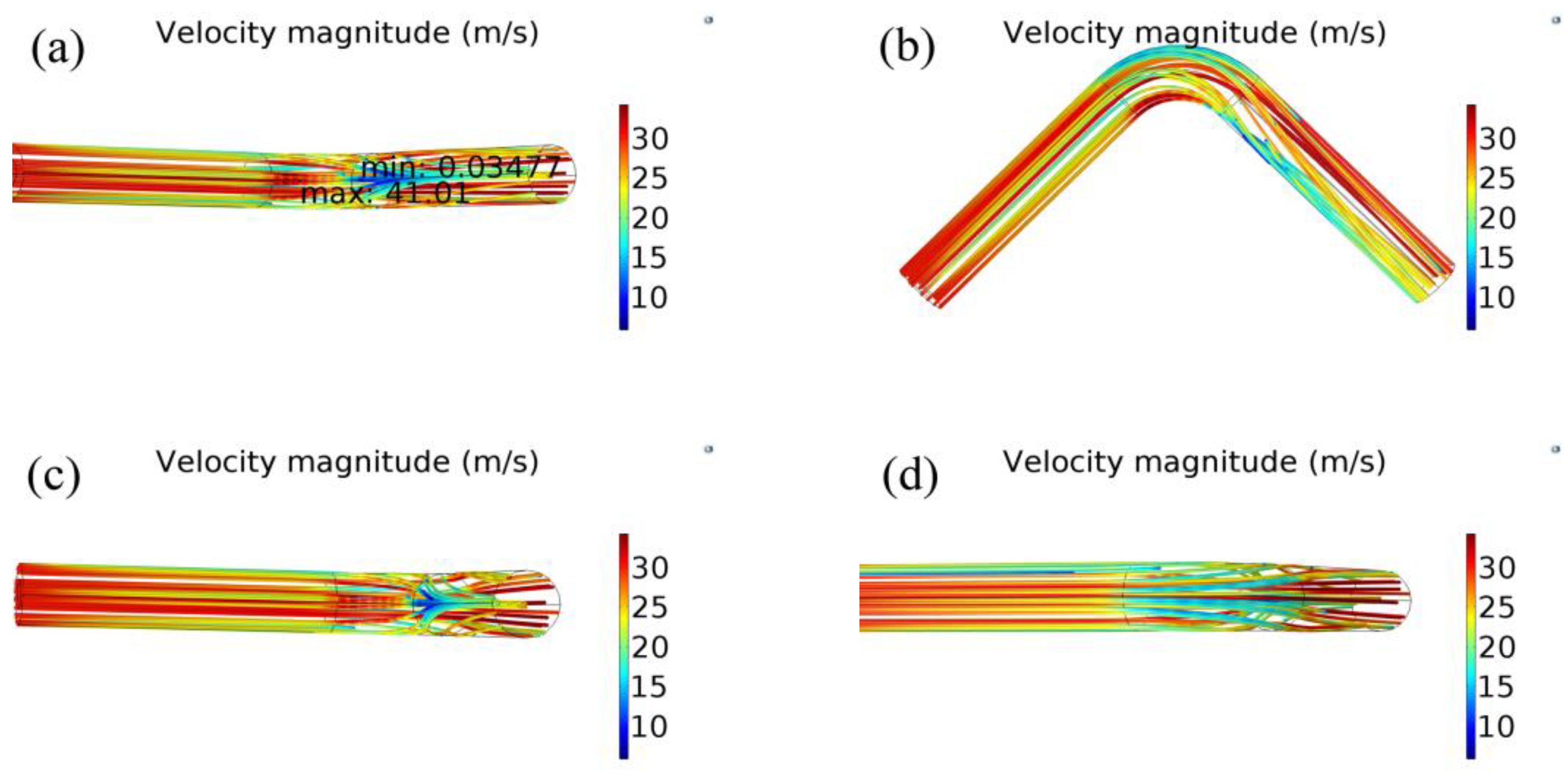
3.1.2. Velocity Streamline in Pipeline
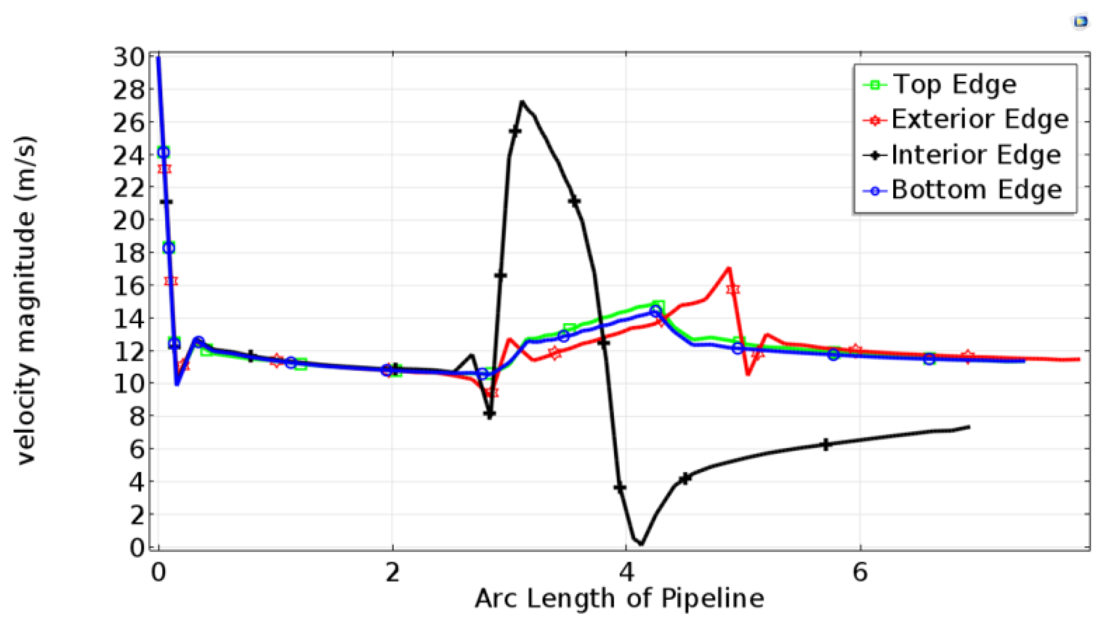
3.1.3. Velocity along the Four Featured Edges
3.2. Electrochemical Corrosion Behavior
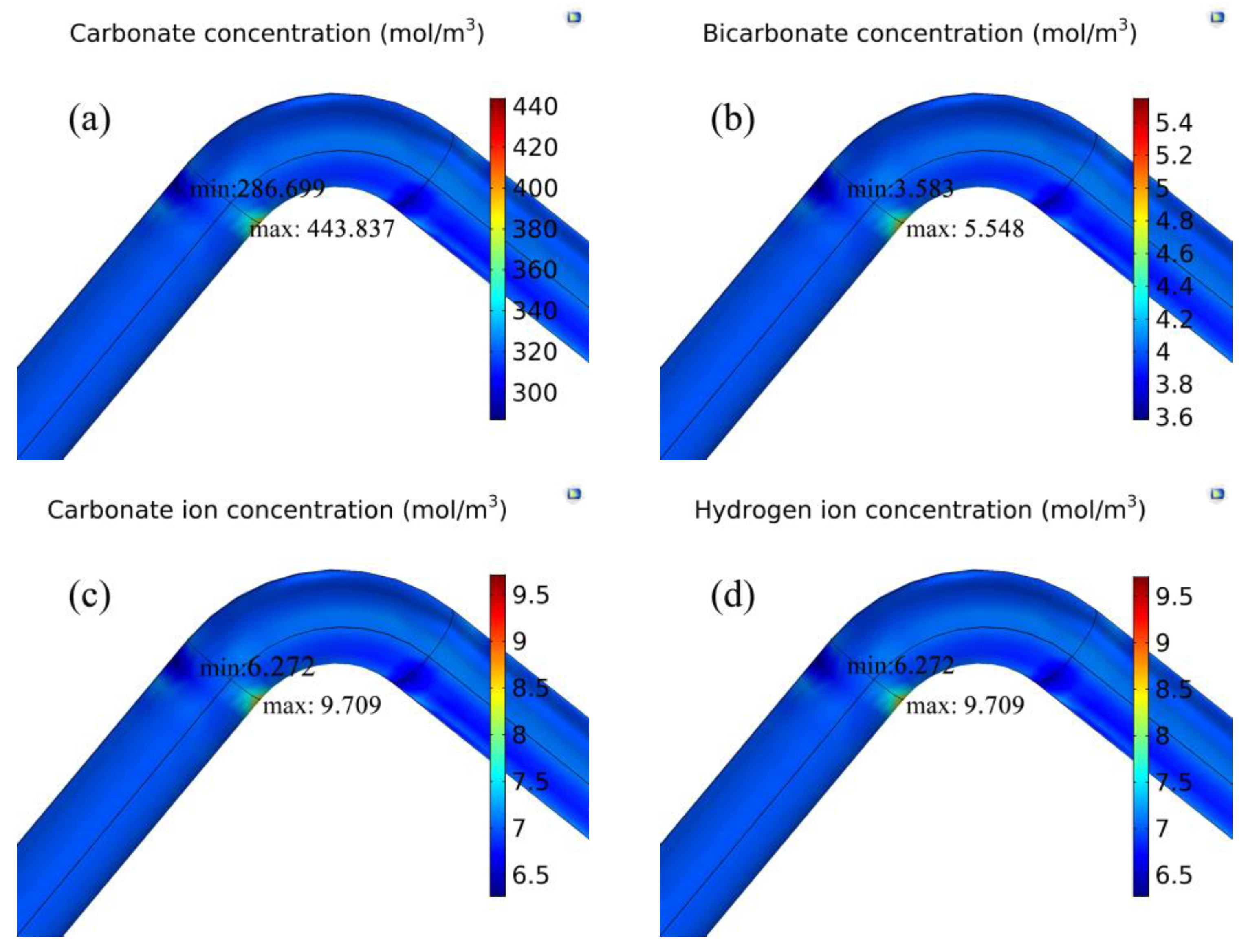
3.2.1. Species Concentration Distribution Characteristic
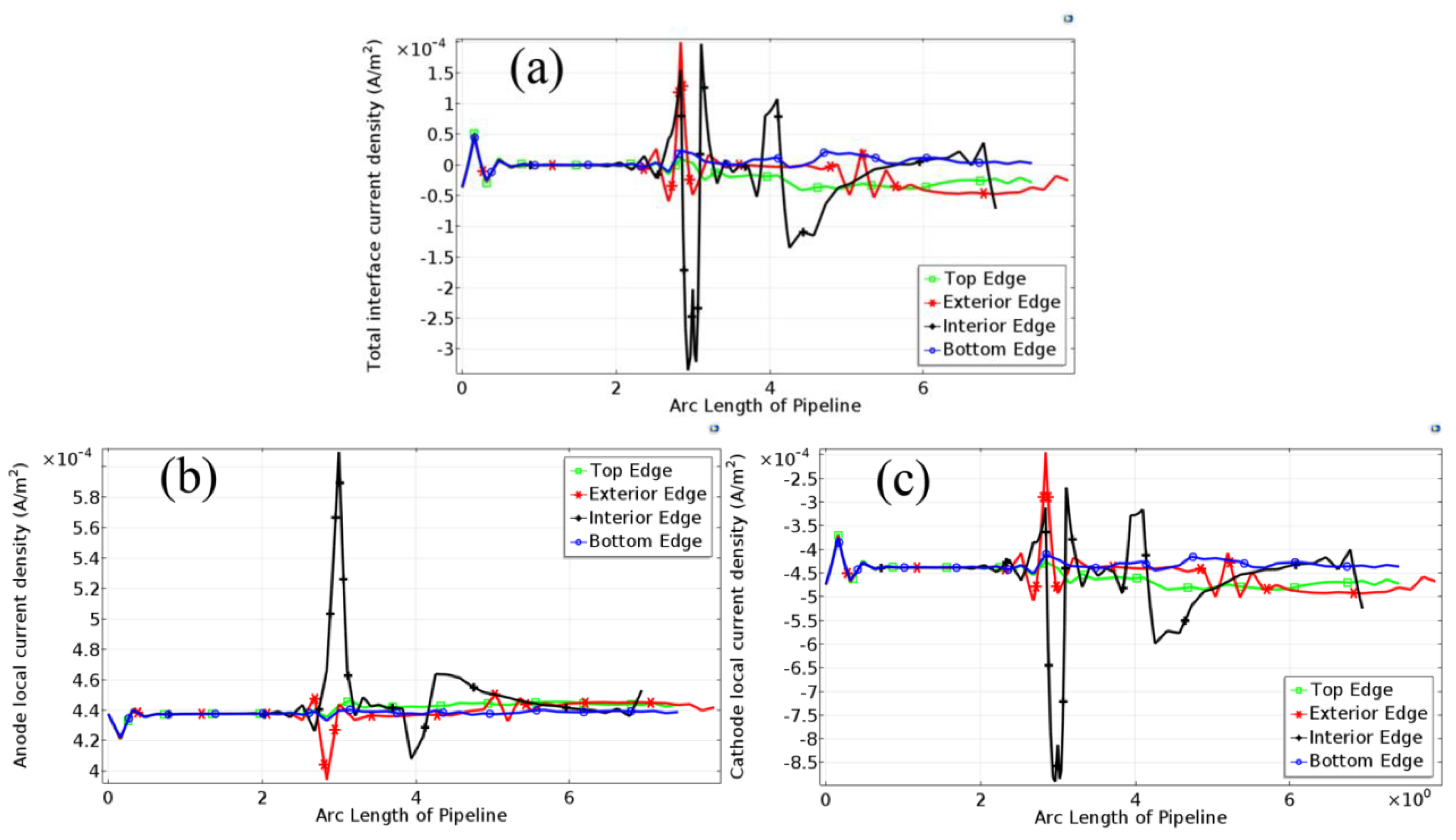
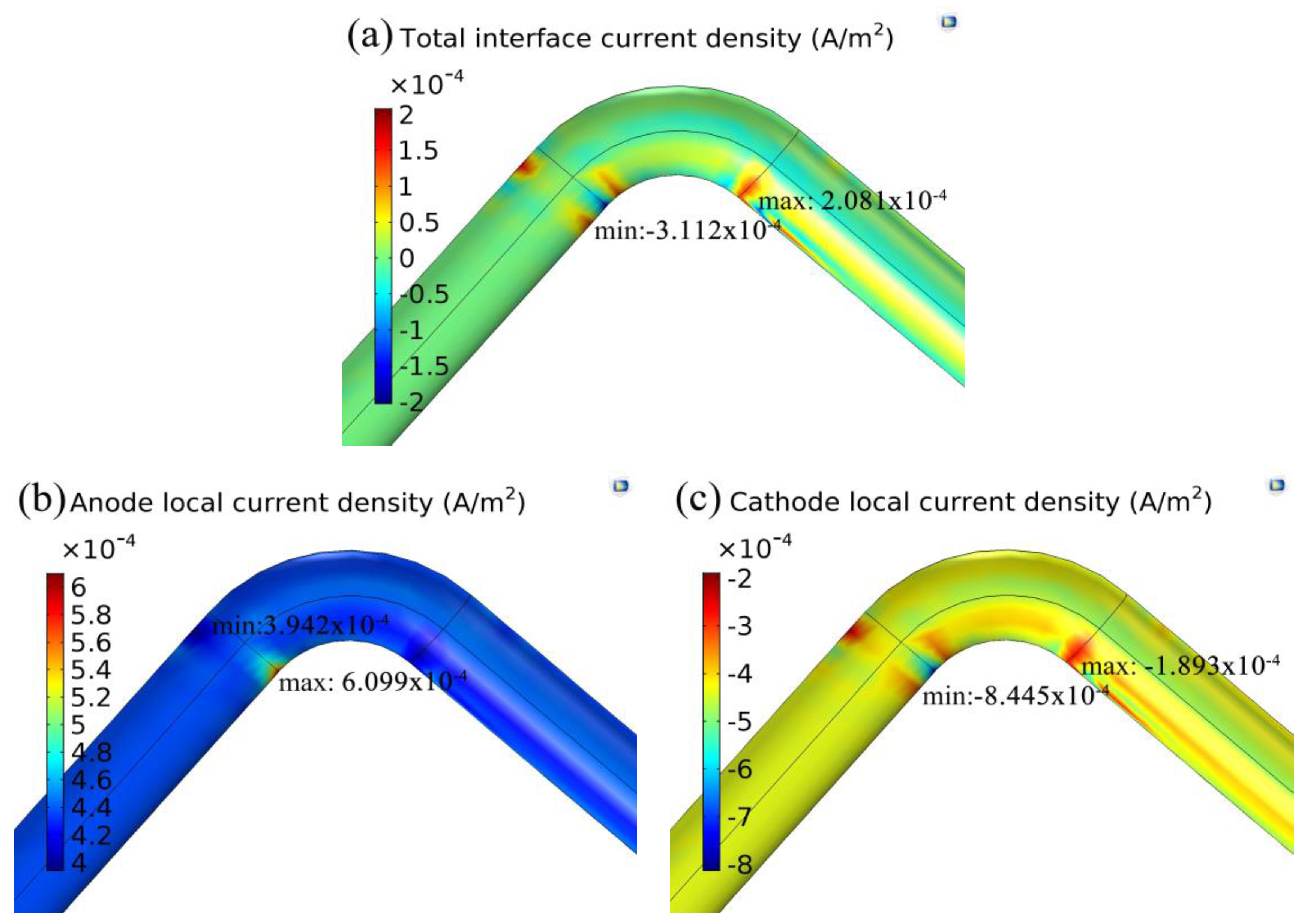
3.2.2. Current Density Characteristic
Total Interface Current Density of Four Edges
Anode Current Density of the Four Edges
Cathode Current Density of the Four Edges
Current Density Distribution on the Wall
3.3. Erosion Behavior
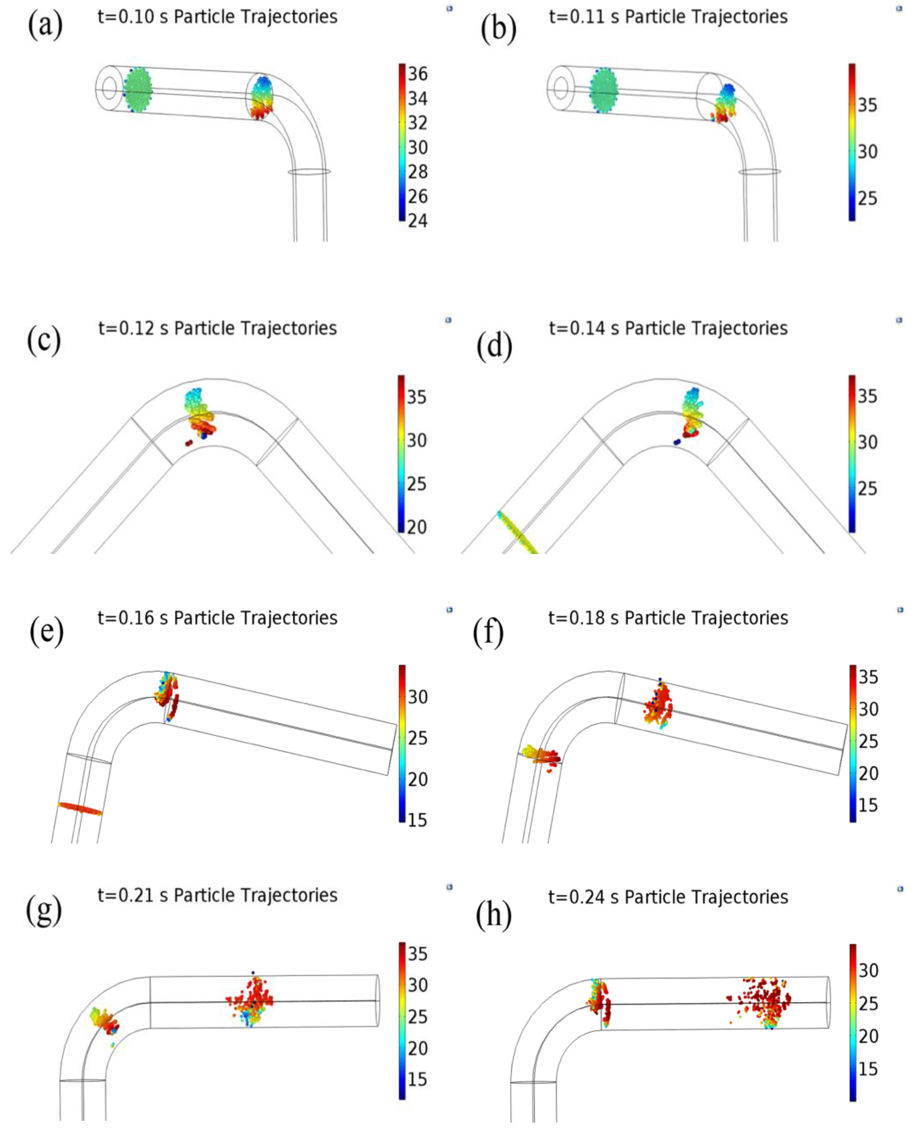
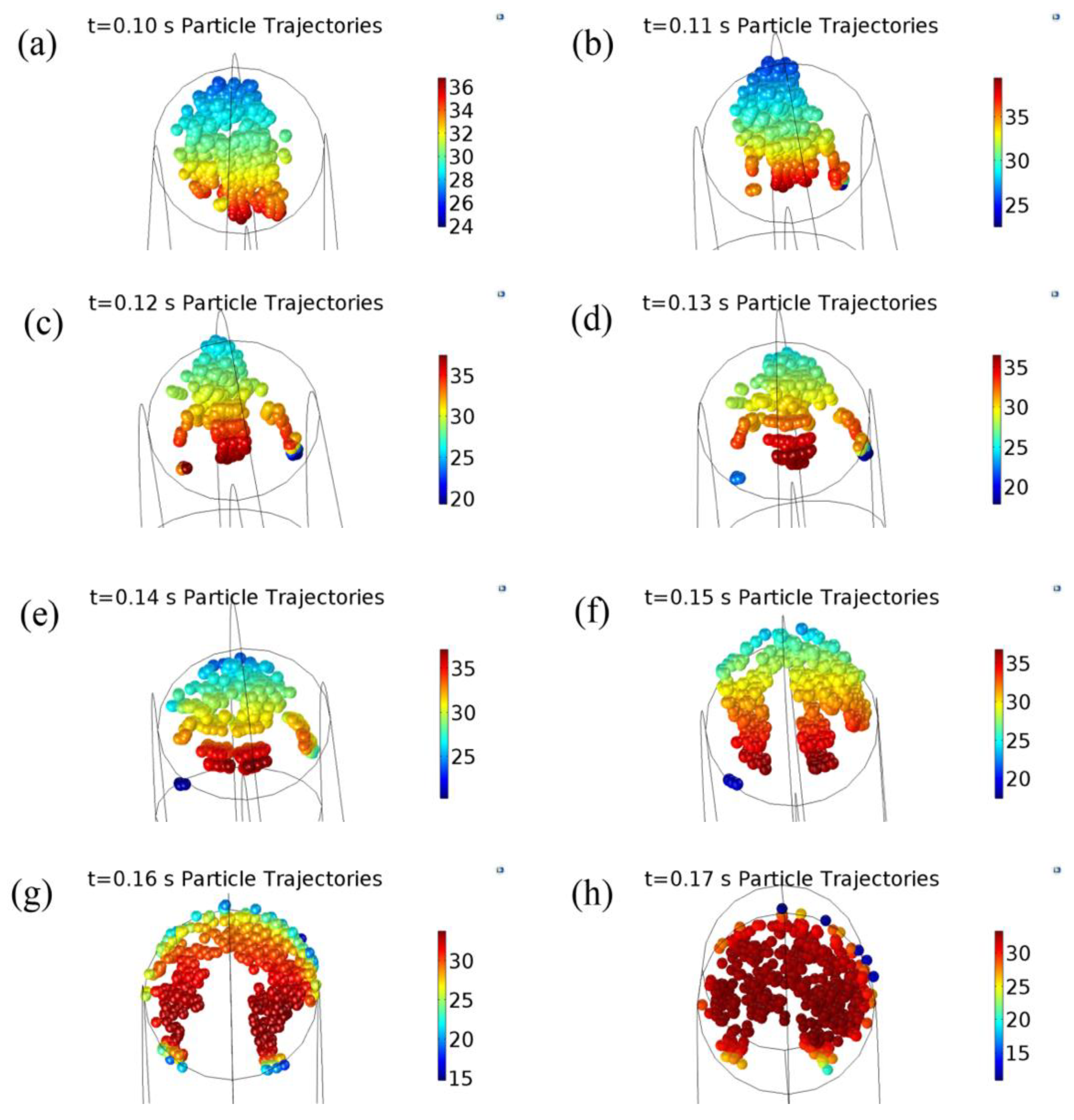
3.3.1. Particle Trajectory
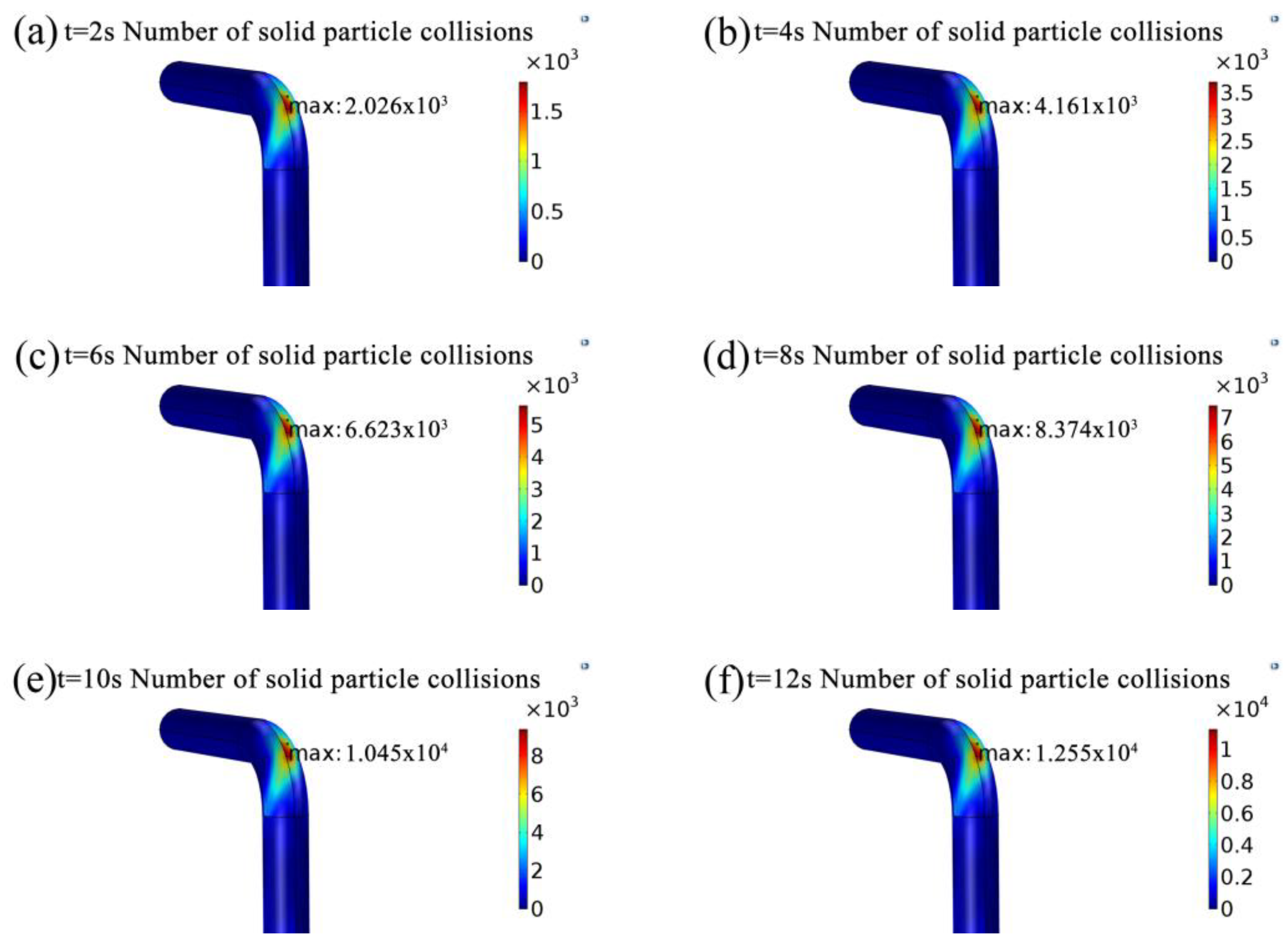
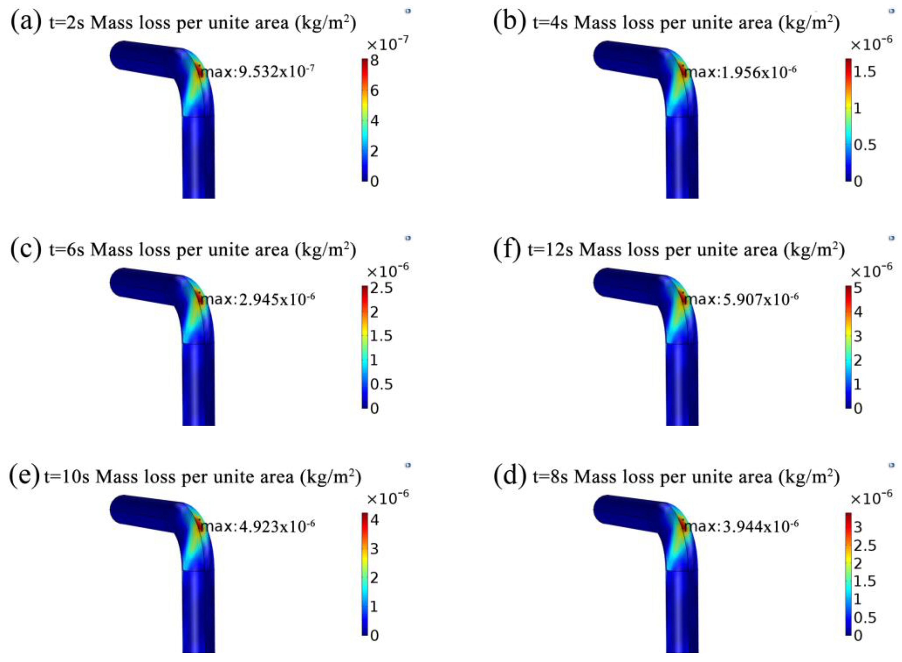
3.3.2. The Quantities of Particles Striking the Wall and Mass Loss Per Unit Area
4. Discussions
4.1. The Correlation between Streamline and Turbulence
4.2. The Correlation of the Electrochemical Corrosion with Material Concentration Distribution
4.3. Erosion in the Turbulence
5. Conclusions
- The serious erosion of elbow occurs between 40° and 50°, and gradually expanded into the surrounding area forming a slanted erosion region under the force, boundary layer’s blocking action and wall rebound. The particles at high speed hit the wall of the tube, especially in the elbow section with high turbulent intensity, which caused the serious erosion area on the extrados of elbow.
- The particles count method is proposed to describe erosion and provide a probability prediction of the elbow lifetime. About 16.7% particles collided the extrados surface during erosion.
- The corrosion current density of iron is concentrated in the junction of the straight section and elbow and the intersection of the straight section and the intrados surface of elbow. The strong turbulent intensity in elbow and the boundary layer affects the substance concentration of chemical reactions accumulated at the junction of the straight section and elbow.
- The pressure on the extrados is higher than that on the intrados. However, the friction speed on the intrados is higher than that on the extrados due to the cumulative effect of gas in pipe. Low viscosity of gas and the geometric constraints are attributed to cause difference in the velocity magnitude and particles hitting the wall in straight line.
Author Contributions
Funding
Acknowledgments
Conflicts of Interest
References
- Rajahram, S.; Harvey, T.; Wood, R. Erosion–corrosion resistance of engineering materials in various test conditions. Wear 2009, 267, 244–254. [Google Scholar] [CrossRef]
- De Waard, C.; Lotz, U.; Milliams, D. Predictive model for CO2 corrosion engineering in wet natural gas pipelines. Corrosion 1991, 47, 976–985. [Google Scholar] [CrossRef]
- Liang, G.; Peng, X.; Xu, L.; Cheng, Y.F. Erosion-corrosion of carbon steel pipes in oil sands slurry studied by weight-loss testing and CFD simulation. J. Mater. Eng. Perform. 2013, 22, 3043–3048. [Google Scholar] [CrossRef]
- Liu, H.; Zhou, Z.; Liu, M. A probability model of predicting the sand erosion profile in elbows for gas flow. Wear 2015, 342, 377–390. [Google Scholar] [CrossRef]
- Zeng, L.; Shuang, S.; Guo, X.P.; Zhang, G.A. Erosion-corrosion of stainless steel at different locations of a 90 elbow. Corros. Sci. 2016, 111, 72–83. [Google Scholar] [CrossRef]
- Finnie, I. Some observations on the erosion of ductile metals. Wear 1972, 19, 81–90. [Google Scholar] [CrossRef]
- Patterson, C.S.; Slocum, G.H.; Busey, R.H.; Mesmer, R.E. Carbonate equilibria in hydrothermal systems: First ionization of carbonic acid in NaCl media to 300 °C. Geochim. Cosmochim. Acta 1982, 46, 1653–1663. [Google Scholar] [CrossRef]
- Nesic, S.; Postlethwaite, J.; Olsen, S. An electrochemical model for prediction of corrosion of mild steel in aqueous carbon dioxide solutions. Corrosion 1996, 52, 280–294. [Google Scholar] [CrossRef]
- Oddo, J.; Tomson, M. Simplified calculation of CaCO3 saturation at high temperatures and pressures in brine solutions. J. Pet. Technol. 1982, 34, 1583–1590. [Google Scholar] [CrossRef]
- Nordsveen, M.; Nešic, S.; Nyborg, R.; Stangeland, A. A mechanistic model for carbon dioxide corrosion of mild steel in the presence of protective iron carbonate films—Part 1: Theory and verification. Corrosion 2003, 59, 443–456. [Google Scholar]
- Kvarekval, J. A kinetic model for calculating concentration profiles and fluxes of CO2-related species across the nernst diffusion layer. In Corrosion 97, March 9–14, 1997; NACE International: New Orleans, LA, USA, 1997. [Google Scholar]
- Newman, J.; Thomas-Alyea, K. Electrochemical Systems; John Wiley & Sons: Hoboken, NJ, USA, 2012. [Google Scholar]
- Zhang, E.; Zeng, D.; Zhu, H.; Li, S.; Chen, D.; Li, J.; Ding, Y.; Tian, G. Numerical simulation for erosion effects of three-phase flow containing sulfur particles on elbows in high sour gas fields. Petroleum 2018, 4, 158–167. [Google Scholar] [CrossRef]
- Xu, Y.; Tan, M. Probing the initiation and propagation processes of flow accelerated corrosion and erosion corrosion under simulated turbulent flow conditions. Corros. Sci. 2019, 151, 163–174. [Google Scholar] [CrossRef]
- Zhao, J.; Xiong, D.; Gu, Y.; Zeng, Q.; Tian, B. A comparative study on the corrosion behaviors of X100 steel in simulated oilfield brines under the static and dynamic conditions. J. Pet. Sci. Eng. 2019, 173, 1109–1120. [Google Scholar] [CrossRef]
- Islam, M.A.; Farhat, Z.N.; Ahmed, E.M.; Alfantazi, A.M. Erosion enhanced corrosion and corrosion enhanced erosion of API X-70 pipeline steel. Wear 2013, 302, 1592–1601. [Google Scholar] [CrossRef]
- Wood, R.J.K.; Wharton, J.A.; Speyer, A.J.; Tan, K.S. Investigation of erosion–corrosion processes using electrochemical noise measurements. Tribol. Int. 2002, 35, 631–641. [Google Scholar] [CrossRef]
- Zeng, L.; Chen, G.; Chen, H. Comparative study on flow-accelerated corrosion and erosion–corrosion at a 90 carbon steel bend. Materials 2020, 13, 1780. [Google Scholar] [CrossRef] [PubMed]
- Stack, M.; Abdelrahman, S.; Jana, B. A new methodology for modelling erosion–corrosion regimes on real surfaces: Gliding down the galvanic series for a range of metal-corrosion systems. Wear 2010, 268, 533–542. [Google Scholar] [CrossRef]
- Liu, J.; BaKeDaShi, W.; Li, Z.; Xu, Y.; Ji, W.; Zhang, C.; Cui, G.; Zhang, R. Effect of flow velocity on erosion–corrosion of 90-degree horizontal elbow. Wear 2017, 376, 516–525. [Google Scholar] [CrossRef]
- Jianwen, Z.; Aiguo, J.; Yanan, X.; Jianyun, H. Numerical investigation on multiphase erosion-corrosion problem of steel of apparatus at a well outlet in natural gas production. J. Fluids Eng. 2018, 140. [Google Scholar] [CrossRef]
- Okhovat, A.; Heris, S.Z.; Asgarkhani, M.H.; Fard, K.M. Modeling and simulation of erosion–corrosion in disturbed two-phase flow through fluid transport pipelines. Arab. J. Sci. Eng. 2014, 39, 1497–1505. [Google Scholar] [CrossRef]


| Number | Number of Mesh Nodes | Max Fluid Velocity (m/s) |
|---|---|---|
| 1 | 21,264 | 41.01 |
| 2 | 31,248 | 41.19 |
| 3 | 61,200 | 41.43 |
| Constant | Source |
|---|---|
| mol | Oddo and Tomson [9] |
| s−1 | Comprehensive chemical kinetics |
| mol | Oddo and Tomson |
| s−1 | Nordsveen [10] |
| DH2CO3 = 2.00 × 10⁻⁹ m2/s | Kvarekval [11] |
| DHCO3− = 1.105 × 10⁻⁹ m2/s | Newman [12] |
| DH+ = 9.312 × 10⁻⁹ m2/s | Newman |
| DCO3 = 0.92 × 10⁻⁹ m2/s | Kvarekval |
| Time | The Total Number of Particles in the Pipeline | The Number of Particles Hitting the Extrados | Statistical Probability of Collision | Maximum of Mass Loss per Unite Area on the Extrados (kg/m2) |
|---|---|---|---|---|
| 2 s | 12,500 | 2026 | 16.2% | 9.53 × 10⁻⁷ |
| 4 s | 25,000 | 4161 | 16.6% | 1.96 × 10⁻⁶ |
| 6 s | 37,500 | 6263 | 16.7% | 2.95 × 10⁻⁶ |
| 8 s | 50,000 | 8374 | 16.75% | 3.94 × 10⁻⁶ |
| 10 s | 62,500 | 10,450 | 16.72% | 4.92 × 10⁻⁶ |
| 12 s | 75,000 | 12,550 | 16.73% | 5.91 × 10⁻⁶ |
© 2020 by the authors. Licensee MDPI, Basel, Switzerland. This article is an open access article distributed under the terms and conditions of the Creative Commons Attribution (CC BY) license (http://creativecommons.org/licenses/by/4.0/).
Share and Cite
Zeng, Q.; Qi, W. Simulation Analysis of Erosion–Corrosion Behaviors of Elbow under Gas-Solid Two-Phase Flow Conditions. Lubricants 2020, 8, 92. https://doi.org/10.3390/lubricants8090092
Zeng Q, Qi W. Simulation Analysis of Erosion–Corrosion Behaviors of Elbow under Gas-Solid Two-Phase Flow Conditions. Lubricants. 2020; 8(9):92. https://doi.org/10.3390/lubricants8090092
Chicago/Turabian StyleZeng, Qunfeng, and Wenchuang Qi. 2020. "Simulation Analysis of Erosion–Corrosion Behaviors of Elbow under Gas-Solid Two-Phase Flow Conditions" Lubricants 8, no. 9: 92. https://doi.org/10.3390/lubricants8090092
APA StyleZeng, Q., & Qi, W. (2020). Simulation Analysis of Erosion–Corrosion Behaviors of Elbow under Gas-Solid Two-Phase Flow Conditions. Lubricants, 8(9), 92. https://doi.org/10.3390/lubricants8090092