Article

Friction-Induced Vibration Suppression via the Tuned Mass Damper: Optimal Tuning Strategy

1
Department of Applied Mechanics, Budapest University of Technology and Economics, 1111 Budapest, Hungary
2
Department of Applied Mechanics, MTA-BME Lendület Machine Tool Vibration Research Group, Budapest University of Technology and Economics, 1111 Budapest, Hungary
*
Author to whom correspondence should be addressed.
Lubricants 2020, 8(11), 100; https://doi.org/10.3390/lubricants8110100
Submission received: 29 October 2020 / Revised: 15 November 2020 / Accepted: 16 November 2020 / Published: 20 November 2020
(This article belongs to the Special Issue Interfacial Dissipative Phenomena in Tribomechanical Systems)

Abstract

:
Friction-induced vibrations are a significant problem in various engineering applications, while dynamic vibration absorbers are an economical and effective tool for suppressing various kinds of vibrations. In this study, the archetypal mass-on-moving-belt model with an attached dynamic vibration absorber was considered. By adopting an analytical procedure, the optimal tuning of the absorber’s parameters was defined. Furthermore, the bifurcations occurring at the loss of stability were analytically investigated; this analysis illustrated that a properly chosen nonlinearity in the absorber’s stiffness permits controlling the supercritical or subcritical character of the bifurcation. However, a numerical analysis of the system’s dynamics, despite confirming the analytical results, also illustrated that the system’s global behavior is only slightly affected by the bifurcation character. Indeed, a dynamic vibration absorber possessing a perfectly linear restoring force function seems to provide the optimal performance; namely, it minimizes the velocity range for which stick–slip oscillations exists.

Graphical Abstract

1. Introduction

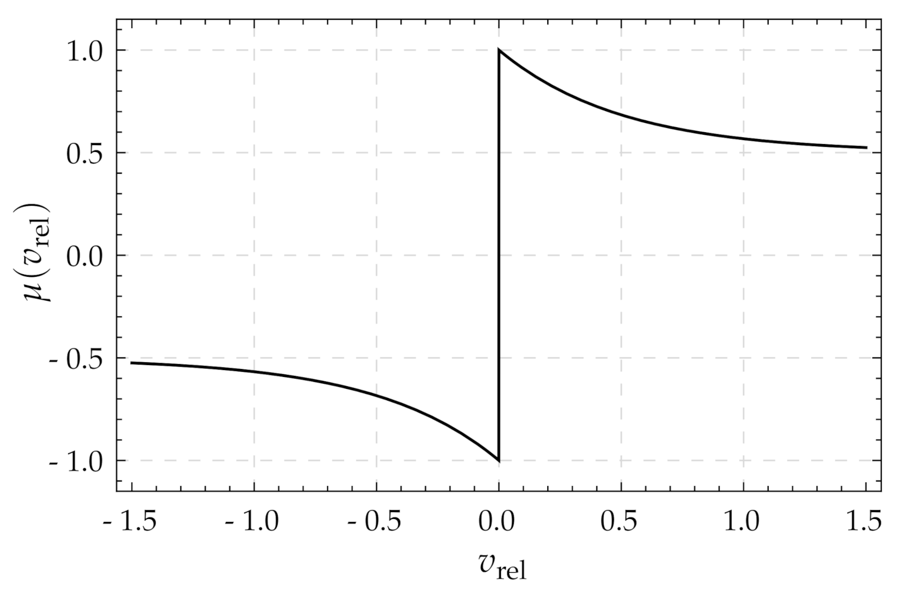
Friction-induced vibrations (FIVs) are a peculiar type of oscillations generated by the friction acting between two bodies in relative motion. They consist of either the successions of stick and slip phases between the two bodies [1], or of quasi-harmonic oscillations having an approximately sinusoidal displacement–time relation [2,3]. Although for some specific applications these kinds of vibrations are intentionally generated, such in the case of violin strings [4] and singing wine glasses [5], typically they are seen as a detrimental phenomenon, as in the cases of brake squeal [6] or earthquakes [7,8].
Several methods exist for suppressing FIVs. One possibility is to reduce the friction force at the interface utilizing a lubricant. This method is efficient if friction is not required for the device to operate, such as in the case of hinge squeaking; however, it cannot be adopted for brake squeal mitigation, where high friction is strictly required. Most brake squeal suppression methods consist of increasing the system damping, which is obtained with various techniques [6,9]. Experimental observations also illustrated that isolating the natural frequencies of the brake system’s components at low frequencies tends to reduce the occurrence of audible brake squeal [10]; however, in many cases, this strategy is not effective [11]. For active methods for suppressing FIV, Cunefare and Graf [12] proposed adopting a dither exciting the system at non-audible frequencies, which can suppress brake squeal. Papangelo and Ciavarella [13] proposed to mitigate FIVs by normal load variation, for which they provided a closed-form solution.
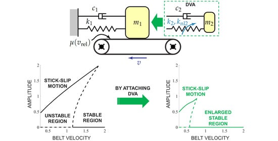
The dynamic vibration absorber (DVA) is a practical tool for suppressing undesired vibrations in several engineering applications. Its classical design [14] consists of a mass attached to the host structure through a spring and a damper. By tuning its natural frequency in correspondence of the frequency to be damped, it is able to dynamically interact with the host structure dissipating vibration energy. It is successfully employed in several engineering fields for the suppression of various kinds of vibrations, such as flutter instabilities [15,16], rolling motions in ships [17], helicopter rotor oscillations [18] and machine tool vibrations [19,20]. Although DVAs are a mature technology, which was first proposed more than one hundred years ago [17], to the authors’ knowledge, there are only a few and relatively recent studies addressing its implementation to suppress FIVs. Popp and Rudolph [21] numerically and experimentally analyzed the performance of a DVA for FIV suppression; by utilizing a single-degree-of-freedom (DoF) primary system, they illustrated its beneficial effect. Chatterjee [22] studied the stability properties of an undamped DVA attached to a two-DoF primary system. Very recently, Niknam and Farhang [23] proposed a study similar to that of Chatterjee [22], where they also provided some numerical simulations of the full system, missing in [22]. Despite the promising results obtained in [21,22,23], a clear tuning strategy of the DVA’s parameters for maximizing its performance is still missing. This paper aims to fill this gap by providing a precise tuning of the absorber parameters for optimizing stability properties and studying the behavior of the host system with the attached DVA while stability is lost.
The rest of the paper is organized as follows. In Section 2, the mechanical model, consisting of the host mass-on-moving-belt system and the attached DVA, is introduced. In Section 3, the stability analysis of the host system, without and with the DVA, is performed, providing explicit equations for the optimal tuning of the absorber parameters. In Section 4 and Section 5, the bifurcations occurring at the loss of stability of the host system, without and with absorber, are analytically studied. Furthermore, the effect of the addition of a cubic term in the absorber’s restoring force is analytically investigated; analytical results are integrated by numerical simulation, illustrating the system’s behavior at high amplitudes. In Section 6, conclusions about the benefits and limitations of the DVA are presented.

2. Mechanical Model

2.1. Primary System

The primary system considered in this study is the classical mass-on-moving-belt model, which is an archetypal system for studying FIVs [1,4,21]. As shown in Figure 1, this single-DoF system consists of a mass m 1 , a linear spring k 1 and a linear damper c 1 . The mass of the system is in contact with the belt, which moves at a constant driving speed v, while the friction coefficient μ ( v rel ) of the contact is a function of the relative velocity v rel = v x ˙ 1 .
Figure 1b illustrates the free body diagram (FBD) of the host system. The forces acting upon the lumped mass m 1 are the normal forces F N that cancel each other; the damping and spring forces F c 1 and F k 1 , respectively; and the friction force F R . (For the represented FBD, it is assumed that v rel 0 .) Based on Newton’s second law of motion and considering that F R = μ ( v rel ) F N , F c 1 = c 1 x ˙ 1 and F k 1 = k 1 x 1 , we obtain that the second order differential equation describing the motion of the one DoF system is
m 1 x ¨ 1 + c 1 x ˙ 1 + k 1 x 1 = F R ,
with
F R = μ ( v rel ) F N v rel 0 | F R | μ s F N v rel = 0 ,
where the overdot indicates derivation with respect to the time t. The system is in stick condition when the relative velocity is zero ( v rel = 0 ). In this case, the friction force is smaller or equal to μ s F N , where μ s is the static friction. In sliding condition ( v rel 0 ), the direction of the friction force F R depends on the sign of the relative velocity v rel , which is included in the mathematical formulation of μ ( v rel ) . Additional details about the friction coefficient utilized are provided in Section 2.3. Let us introduce the following expressions
ζ 1 = c 1 2 m 1 k 1 ;   ω n 1 = k 1 m 1   ;   x 0 = F N k 1   ;   τ = ω n 1 t   .
By dividing Equation (1) by the mass m 1 , applying the expressions from Equation (3) and dividing it by ω n 1 2 , we obtain
x 1 + 2 ζ 1 x 1 + x 1 = F R k 1   ,
where prime indicates derivation with respect to the dimensionless time τ . Then, introducing the dimensionless displacement x ˜ 1 = x 1 / x 0 , the system is eventually reduced to
x ˜ 1 + 2 ζ 1 x ˜ 1 + x ˜ 1 = F ˜ R   ,
where F ˜ R = F R / F N .

2.2. Mechanical Model of the Host System with the Absorber

We now attach a DVA to the host system. The basis of the model is the same as the one mentioned in the previous subsection. The only additional element is the absorber mass m 2 , which is attached to the primary system through a spring and a linear damper. The schematic depiction of this two-DoF system is provided in Figure 2.
The absorber’s spring encompasses a linear term and a cubic term. The differential equations describing the dynamics of the system are
m 1 x ¨ 1 + c 1 x ˙ 1 + k 1 x 1 + c 2 ( x ˙ 1 x ˙ 2 ) + k 2 ( x 1 x 2 ) + k nl 2 ( x 1 x 2 ) 3 = F R m 2 x ¨ 2 + c 2 ( x ˙ 2 x ˙ 1 ) + k 2 ( x 2 x 1 ) + k nl 2 ( x 2 x 1 ) 3 = 0   ,
where k 2 and k nl 2 are the linear and cubic coefficients of the absorber stiffness, respectively, while c 2 is the linear coefficient of the absorber damping. Let us introduce the following expressions
ζ 2 = c 2 2 m 2 k 2   ;   ω n 2 = k 2 m 2   ;   ε = m 2 m 1   ;   γ = ω n 2 ω n 1   .
By diving Equation (6) by m 1 , applying the expressions from (7) and (3), dividing by ω n 1 2 and utilizing the dimensionless time τ and dimensionless displacements x ˜ 1 and x ˜ 2 = x 2 / x 0 , we obtain
x ˜ 1 + 2 ζ 1 x ˜ 1 + x ˜ 1 + 2 ε ζ 2 γ ( x ˜ 1 x ˜ 2 ) + ε γ 2 ( x ˜ 1 x ˜ 2 ) + ε κ nl 2 ( x ˜ 1 x ˜ 2 ) 3 = F ˜ R ε x ˜ 2 + 2 ε ζ 2 γ ( x ˜ 2 x ˜ 1 ) + ε γ 2 ( x ˜ 2 x ˜ 1 ) + ε κ nl 2 ( x ˜ 2 x ˜ 1 ) 3 = 0   ,
where κ nl 2 = k nl 2 x 0 2 / ( k 1 ε ) . A variable change is performed, where x ˜ 3 = x ˜ 1 x ˜ 2 (relative displacement of m 2 ), hence Equation (8) transforms into
x ˜ 1 + 2 ζ 1 x ˜ 1 + x ˜ 1 + 2 ε ζ 2 γ x ˜ 3 + ε γ 2 x ˜ 3 + ε κ nl 2 x ˜ 3 3 = F ˜ R ε ( ( x ˜ 1 x ˜ 3 ) 2 ζ 2 γ x ˜ 3 γ 2 x ˜ 3 κ nl 2 x ˜ 3 3 ) = 0   .

2.3. Friction Force

The applied friction law is described by an exponential decaying function, as done for instance in [1], i.e.,
μ ( v rel ) = ( μ d + ( μ s μ d ) e | v rel | v ˜ 0 ) sgn ( v rel )   ,
where the relative velocity is v rel = v x ˜ 1 . The values assumed by μ for a range of relative velocities for μ s = 1 , μ d = 0.5 and v 0 = 0.5 are represented in Figure 3. The values for the friction law adopted in the present study are the same utilized in [1]. Nevertheless, as illustrated below, the optimization of the absorber parameters does not strictly depend on the considered friction law.

3. Linear Stability Analysis

We now aim at analyzing the system’s behavior for small perturbations around the equilibrium. Thus, we linearize it around its trivial solution and we study the stability of this trivial solution. The analysis is performed for both the systems, with and without DVA, in order to assess the beneficial effects of the DVA.

3.1. Linear Stability of the Host System without the DVA

We first linearize Equation (5) around its equilibrium point x 1 e = μ ( v rel = v ) , obtaining
z 1 2 ψ z 1 + z 1 = 0   ,
where z 1 = x 1 e + x ˜ 1 and 2 ψ = μ / z 1 | z 1 = 0 2 ζ 1 . Considering the friction law adopted, we have that
μ z 1 | z 1 = 0 = μ s μ d v 0 e v v 0   ,
(valid for v > 0 ), which is the slope of the friction force coefficient at the belt velocity v.
Equation (11) corresponds to a linear oscillator, whose trivial solution is asymptotically stable if and only if ψ < 0 . According to the friction law utilized, and considering that ψ is a monotonically decreasing function of v, the trivial solution is stable for
v > v h , cr = v 0 ln μ s μ d 2 v 0 ζ 1   .
This result is well-known and better discussed, for instance, in [1]. The practical consequences are that, if the belt moves at a speed lower than v h , cr , the equilibrium of the system is unstable and stick–slip oscillations occur. More details about these stick–slip oscillations are provided below.

3.2. Linear Stability of the Host System with DVA

To study the stability of the system with the DVA, we linearize Equation (9) around the equilibrium x ˜ 1 = x 1 e and x ˜ 3 = 0 . By reformulating Equation (9) in explicit form with respect to x ˜ 1 and x ˜ 3 and by utilizing the variables and parameters introduced in the previous subsection, we obtain
z 1 z 2 z 3 z 4 = 0 0 1 0 0 0 0 1 1 γ 2 ε 2 ψ 2 ε ζ 2 γ 1 γ 2 ( ε + 1 ) 2 ψ 2 ( ε + 1 ) γ ζ 2 z 1 z 2 z 3 z 4 = Az   ,
where z 1 = x 1 e + x ˜ 1 , z 2 = x 3 , z 3 = z 1 and z 4 = z 2 .
We analyze the characteristic exponents of the system to determine the stability. The characteristic polynomial is
p ( λ ) = det ( A λ I ) = 0   .
The characteristic polynomial is in the form of
p ( λ ) = a 0 λ 4 + a 1 λ 3 + a 2 λ 2 + a 3 λ + a 4 = 0   ( a 0 > 0 )   .
The stability is determined based on the Liénard–Chipart conditions (LCC) [24]. For the polynomial p ( λ ) to have all roots with negative real parts, it is necessary and sufficient that the coefficients of the polynomial are all positive ( a i > 0 , i = 1 , , 4 ) and that the determinant inequalities Δ 1 > 0 and Δ 3 > 0 (Hurwitz determinantal inequalities) are verified, which in our case means
a 0 = 1 > 0   ,
a 1 = 2 ( γ ( 1 + ε ) ζ 2 ψ ) > 0 ψ < ( 1 + ε ) γ ζ 2   ,
a 2 = 1 + γ ( γ ( 1 + ε ) 4 ζ 2 ψ ) > 0 ψ < 1 + γ 2 ( 1 + ε ) 4 γ ζ 2   ,
a 3 = 2 γ ( ζ 2 γ ψ ) > 0 ψ < ζ 2 γ   ,
a 4 = γ 2 > 0   ,
Δ 1 = a 1 = 2 γ ( 1 + ε ) ζ 2 2 ψ > 0   ( Already   present   in   ( 18 ) )   ,
Δ 3 = a 1 a 2 a 3 a 0 a 3 2 a 1 2 a 4 = 4 γ γ 4 ( ε + 1 ) 2 ζ 2 ψ γ 3 ψ 2 ( 4 ( ε + 1 ) ζ 2 2 + ε ) + 2 γ 2 ζ 2 ψ ( 2 ( ε + 1 ) ζ 2 2 + 2 ψ 2 1 ) γ ζ 2 2 ( ε + 4 ψ 2 ) + ζ 2 ψ   > 0   .

3.2.1. Analytical Optimal Solution

Considering the stability analysis performed in the previous section, we aim at finding the parameter values of the absorber which maximize the stable region. The linear system in Equation (14) has the same mathematical form as the one studied in [25]. Thus, we can follow the same steps in order to optimize the absorber.
First, we look at the curves where the coefficients and the Hurwitz determinants are zeros; these are the boundaries where certain roots change. At certain boundaries, the stable/unstable transition takes place. Following the steps discussed in [25], we can define specific points on these curves, which helps us find the optimal parameters. Figure 4 shows the stability regions for different values of ζ 2 ; the boundary curves of the LCC are also depicted. The gray shaded region is the stable region; we can observe that the stability boundary is not at a constant value of ψ as it is the case for the host system without the DVA; instead, it is a function of γ , with a pronounced peak for γ 1 . This is an expected feature, considering that the DVA usually needs to be tuned at a frequency close to the natural frequency of the primary system [14]. For different values of ζ 2 , the maximum value of ψ also changes, thus we need to find the optimal combination of ( ζ 2 , γ ) such that the value of ψ generating instabilities is maximized. For the optimization, the mass ratio ε is assumed constant; however, the results of the analysis show that larger values of ε increase the stable region.
As we can see in Figure 4a, the intersection of the curves a 1 = Δ 1 = 0 and a 3 = 0 defines a point that we denote with C. Its coordinates in the ( ψ , γ ) plane are C = ( ζ 2 1 + ε , 1 / 1 + ε ) . For low values of ζ 2 , Point C marks the maximal value of ψ providing stability, which we call ψ * . Increasing the value of ζ 2 , Figure 4c illustrates that Point C does not identify any more ψ * and that the stability boundary is defined by Equation Δ 3 = 0 . Nevertheless, also for large damping ζ 2 , the value of γ which maximizes ψ * is very close to the γ coordinate of Point C. Therefore, we define Point P as the point of the curve Δ 3 = 0 having the same γ coordinate as C. Substituting the γ coordinate of C, γ = 1 / 1 + ε , into Δ 3 = 0 , we obtain Point P = ( ε / ( 4 ζ 2 1 + ε ) , 1 / 1 + ε ) .
Since Points C and (approximately) P alternatively mark ψ * , depending on the value of the absorber damping ζ 2 , by choosing ζ 2 such that P and C coincide, we can maximize ψ * . Imposing equality between the ψ coordinates of C and P, we attain
ζ 2 1 + ε = ε ( 4 1 + ε ζ 2 )   ,
therefore, ψ * is maximized for
γ = γ opt = 1 1 + ε   and   ζ 2 = ζ 2 opt = 1 2 ε 1 + ε   ,
and the corresponding maximal value of ψ * is
ψ max = ε 2   .
Accordingly, if γ = γ opt and ζ 2 = ζ 2 opt , the system is stable if 2 ψ < ε , or, in other words, if
μ s μ d v 0   e v v 0 2 ζ 1 < ε   .
Considering that ψ is a monotonically decreasing function of v, the equilibrium of the system is stable if
v > v cr = v 0 log μ s μ d v 0 ( ε + 2 ζ 1 )   .
The stability chart corresponding to this case is illustrated in Figure 4b. We remark that the optimal tuning proposed here does not strictly depend on the friction law considered, which could be modeled with alternative functions without varying γ opt and ζ 2 opt . This represent a clear advantage in the case of real engineering applications.

3.2.2. Numerical Validation

The optimization procedure utilized in the previous section is based on a heuristic approach, which does not prove that γ opt and ζ 2 opt provide the maximal possible value of ψ * . Therefore, its validity should be verified numerically. The numerical analysis is performed by directly computing eigenvalues of matrix A on a grid of the ( ζ 2 , γ , ψ ) space for a fixed ε value ( ε = 0.05 ) and identifying the couple of values ζ 2 , γ which provides the maximal ψ * . After several trials, the analysis is finally performed on the grid described in Table 1.
This analysis provided the optimal values for ζ 2 and γ , which are indicated in Table 2 and directly compared with the optimal values obtained analytically.
Although numerical and analytical optimal parameters do not coincide, their difference is minimal and negligible for most engineering applications. In particular, the optimal γ value is practically the same in both cases. The critical velocity, computed utilizing the parameter values indicated in Table 3, has a difference of less than 0.4% in the two cases. We remark that the difference between numerical and analytical computation is not related to the inaccuracy of stability estimation through the LCC, which exactly predicts an equilibrium’s stability, but to the heuristic approach utilized for the optimization.
Figure 5, illustrating the curve Δ 3 = 0 for various values of ζ 2 , enables us to understand the reason for the difference between the results obtained with the numerical and analytical approach. The blue line in the figure corresponds to the analytical optimization, while the green line to the numerical one. The yellow and red curves refer to values of ζ 2 slightly higher and lower than the optimal ones, respectively. The inaccuracy of the analytical procedure is due to the fact that the peak of the Δ 3 = 0 curve does not exactly lie on Point P (which has a fixed γ value and it is not represented in the figure). However, considering the minimal difference found and the practical compactness of Equations (24) and (25), these will be utilized in the continuation of the paper.

3.3. Evaluation of the Absorber’s Performance

We now aim at evaluating the performance of the DVA by performing various comparison between the system with and without DVA. As mentioned above, the critical velocities for both cases are
v h , cr = v 0 ln μ s μ d 2 v 0 ζ 1   ,
v cr = v 0 ln μ s μ d v 0 ( ε + 2 ζ 1 )   .
Considering the characteristics of a logarithm function, we can state that, if the argument becomes 1, the logarithm function yields 0. Thus, there is a certain parameter set for which the critical velocity becomes 0 (inherent stability). We define ζ 1 , cr as the critical primary damping parameter, for which the critical velocity becomes 0. To obtain ζ 1 , cr , we solve the arguments of the logarithm functions for 1; these yield
μ s μ d 2 v 0 ζ 1 h , cr = 1 ζ 1 h , cr = μ s μ d 2 v 0   ,
μ s μ d v 0 ( ε + 2 ζ 1 , cr ) = 1 ζ 1 , cr = μ s μ d v 0 ε 2 v 0   .
Utilizing values in Table 3, the numerical values for the critical primary damping are
ζ 1 h , cr = 0.5   ,
ζ 1 , cr = 0.388197   .
This shows that the application of an optimally tuned DVA with a mass of only 5% of the host system mass enables to reduce the critical primary damping of 22%.
Considering, instead, the critical velocity as a base of comparison, we define the improvement factor φ such that
φ : = v ˜ h , cr v ˜ cr v ˜ h , cr × 100 %   .
The critical velocities for both cases and the improvement factor are plotted against the varying ζ 1 in Figure 6, utilizing the parameter values in Table 3. We can observe that the difference in critical velocity is more significant for smaller values of ζ 1 , i.e., for a slightly damped host system. We also notice that, if the host system is completely undamped, then the critical velocity is undefined, meaning that the equilibrium is always unstable. For any value of the host system damping ζ 1 , the improvement factor is almost always above 50%.
Let us also observe what happens if we vary the value of the mass ratio ε . Similar to before, the critical velocities for both systems and the improvement factor curve are illustrated in Figure 7. The parameter values are those indicated in Table 3. The critical velocity of the host system is constant because it does not depend on ε ; however, for the system with the DVA, the critical velocity monotonously decreases with ε . Utilizing the parameter values in Table 3, the critical velocities for both the host system and the system with DVA are v h , cr = 1.151 and v cr = 0.5641 , hence the improvement provided by the DVA is of φ = 51 % .

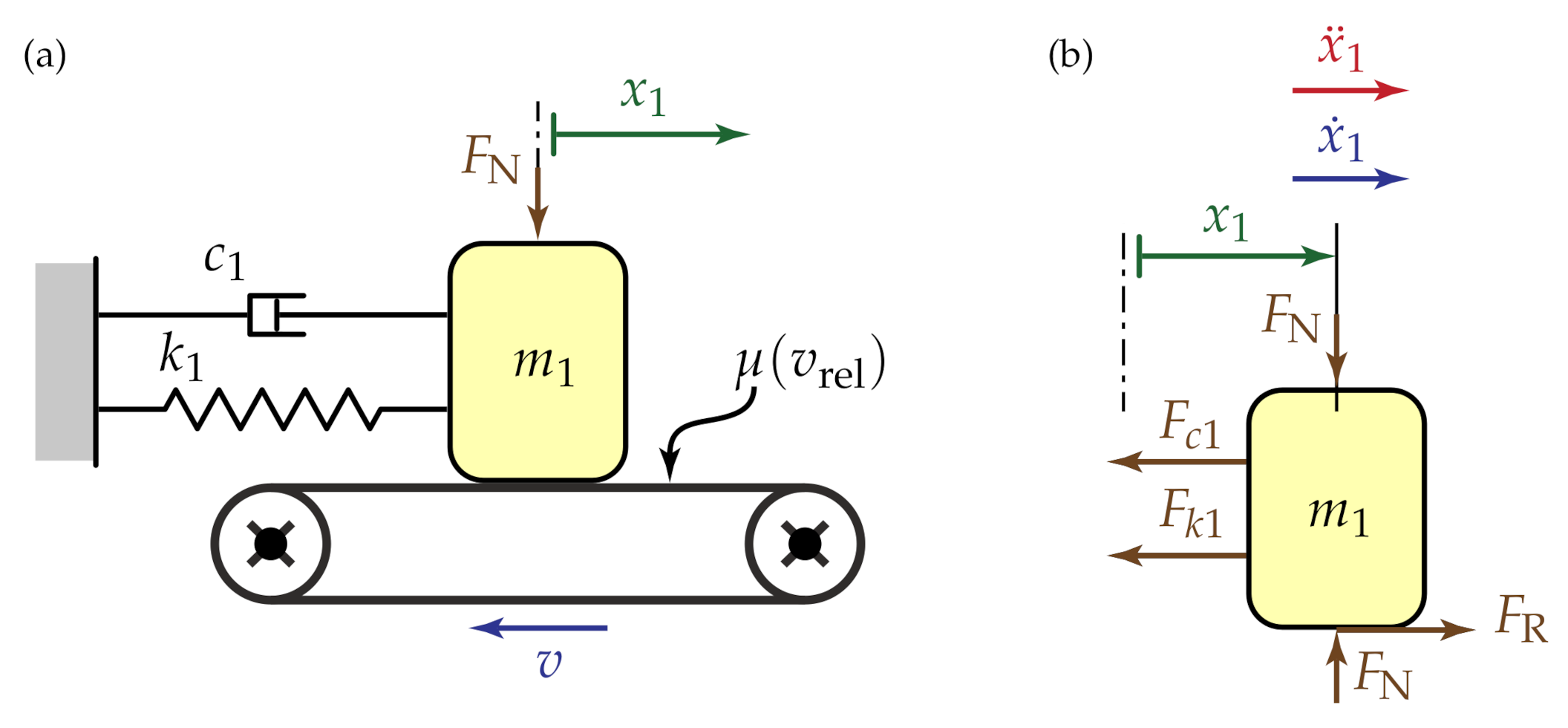
4. Bifurcation Analysis of the Host System without the DVA

The analysis performed in Section 3 refers to the system linearized around its equilibrium. Therefore, it is able to describe its dynamics only in the vicinity of the equilibrium, while phenomena occurring when the stability is lost are overlooked. Additionally, it provides no information about the stable equilibrium’s robustness if the system is subject to non-small perturbations. To investigate the system behavior at the loss of stability and correctly evaluate the DVA performance, we reintroduce the nonlinear terms and analytically perform a bifurcation analysis of the system without and with DVA.
Considering the system in Equation (5), we first center the system around its equilibrium point x 1 e by introducing the variable z 1 = x 1 e + x ˜ 1 , and then we expand it in Taylor series up to the third order, obtaining
z 1 z 3 = 0 1 1 μ d μ s v 0 e v v 0 2 ζ 1 z 1 z 3 + 0 ( μ d μ s 2 v 0 2 e v v 0 ) z 3 2 ( μ d μ s 6 v 0 3 e v v 0 ) z 3 3 = A h z h + b h   .
For v v h , cr , matrix A h has complex conjugate eigenvalues λ 1 , 2 h = α 1 h ± i ω 1 h and eigenvectors s 1 = s ¯ 2 , which are reduced to
λ 1 h = i ,   λ 2 h = i ,   s 1 = i 1 ,   s 2 = i 1  
for v = v h , cr .
We then define the transformation matrix
T h = Re ( s 2 ) Im ( s 2 ) | v = v h , cr   ,
we apply the transformation z = T h y h and we pre-multiply Equation (36) by T h 1 , leading to
y h = T h 1 A h T h y h + T h 1 b h = W h y h + b ˜ h   ,
where
W h = α 1 h ( v ) 1 1 α 1 h ( v )     and     b ˜ h = ( μ d μ s 2 v 0 2 e v v 0 ) y 2 2 ( μ d μ s 6 v 0 3 e v v 0 ) y 2 3 0 .
For v = v h , cr , α 1 h = 0 , α 1 h is kept as a generic function of v, since α 1 h is the critical term causing the instability. The system in Equation (39) is in the so-called Jordan normal form.
By performing several transformations, namely transformation in complex form, near-identity transformation and transformation in polar coordinates, the bifurcation can be characterized through its normal form
r = α 1 h ( v ) r + δ h r 3   ,
where
δ h = e v v 0 ( μ s μ d ) 16 v 0 3   .
Details of this standard procedure can be found in [26]. Non-zero real equilibrium solutions of Equation (41) correspond to periodic motion of the system in Equation (5). Linearizing α 1 h ( v ) around v = v h , cr , we obtain
r = r ( α 1 h * ( v v h , cr ) + δ h r 2 ) ,     where     α 1 h * = d α 1 h d v | v = v h , cr = e v v 0 μ s μ d 2 v 0 2   ,
which has solutions
r = r h 0 = 0     and     r = r h * = α 1 h * ( v v h , cr ) δ h = 2 2 v 0 ( v v h , cr )   .
The trivial solution r h 0 exists for any value v and it is stable for v > v h , cr . Differently, r h * is real only if the argument of the square root in Equation (44) is non-negative, which occurs for v > v h , cr . Since μ s > μ d , in all relevant cases δ is positive (see Equation (42)), which, as clearly explained in [26], means that the bifurcation is subcritical. This implies that r h * corresponds to unstable solutions of Equation (41). This result is in accordance with [1].
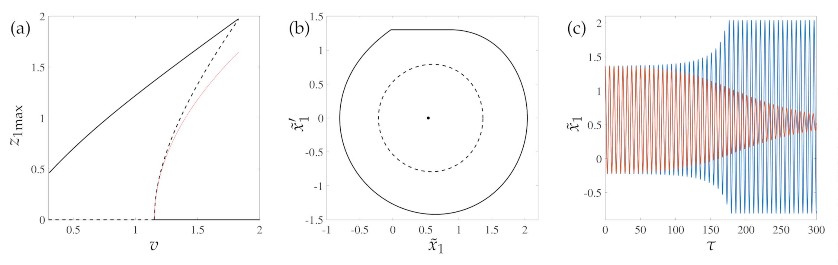
A practical consequence of the subcritical character of the bifurcation is that the system, even within the stable region of the equilibrium ( v > v h , cr ), can experience large oscillations. If the system, while in equilibrium, is subject to a sufficiently large perturbation, which makes it cross the unstable periodic solution in the phase space, it will leave its basin of attraction and it will reach another attractor, which in this case consists of stick–slip oscillations.
The bifurcation diagram in Figure 8a clearly illustrates this scenario. The dashed line indicates a branch of unstable periodic solutions generated at the bifurcation (this branch was obtained through time reverse numerical simulations). The solid line, instead, marks the branch of stick–slip oscillation. The thin solid red line represents the branch of unstable periodic solutions obtained from the analytical computation. We remark on the excellent agreement of the analytically computed solution with the numerical one at low amplitudes. For v ( 1.15 ,   1.83 ) , the system presents two stable solutions, the trivial one and a stick–slip periodic solution, and an unstable periodic solution, as illustrated in Figure 8b for v = 1.3 . Depending on the initial conditions, the system will either converge towards the trivial solution (red curve in Figure 8c) or will undergo stick–slip oscillations (blue curve in Figure 8c). Numerical solutions were computed utilizing the switch model proposed in [4].

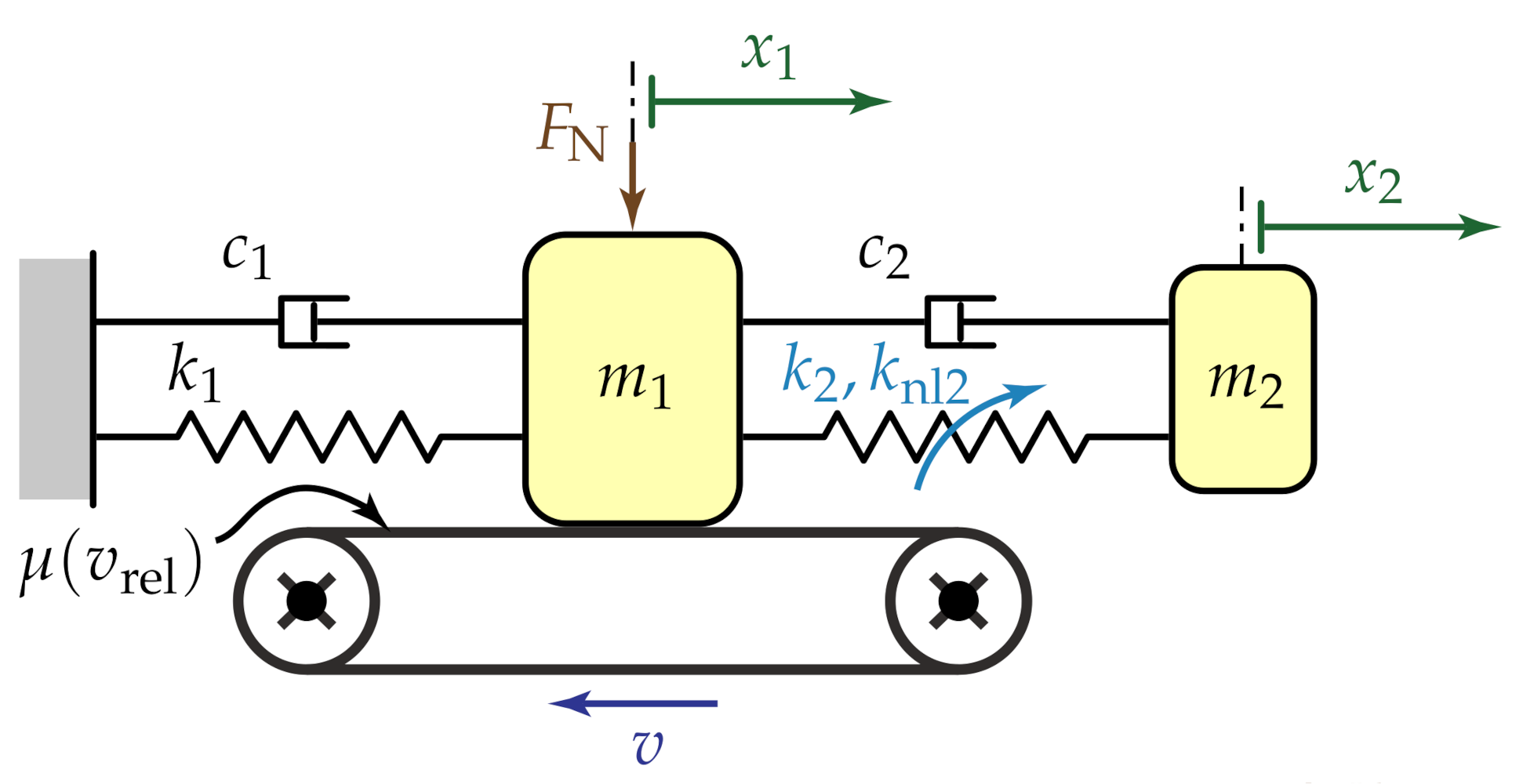
5. Bifurcation Analysis of the Host System with the DVA

To evaluate the DVA performance when stability is lost, we analyze the bifurcation behavior of the system with an attached DVA. The analysis is performed assuming that γ and ζ 2 are tuned approximately according to Equation (25). An analysis of the eigenvalues of matrix A illustrates that at the loss of stability, if γ and ζ 2 are tuned approximately according to Equation (25), a couple of complex conjugate eigenvalues leaves the left-hand side of the complex plane, meaning that their real parts become positive. This scenario corresponds to the occurrence of a Hopf bifurcation. We also notice that, if ζ 2 ζ 2 opt and γ = γ opt , not one, but two couples of complex conjugate eigenvalues leave the left-hand side of the complex plane. Referring to the stability chart in Figure 4a, the entire unstable region matrix A 
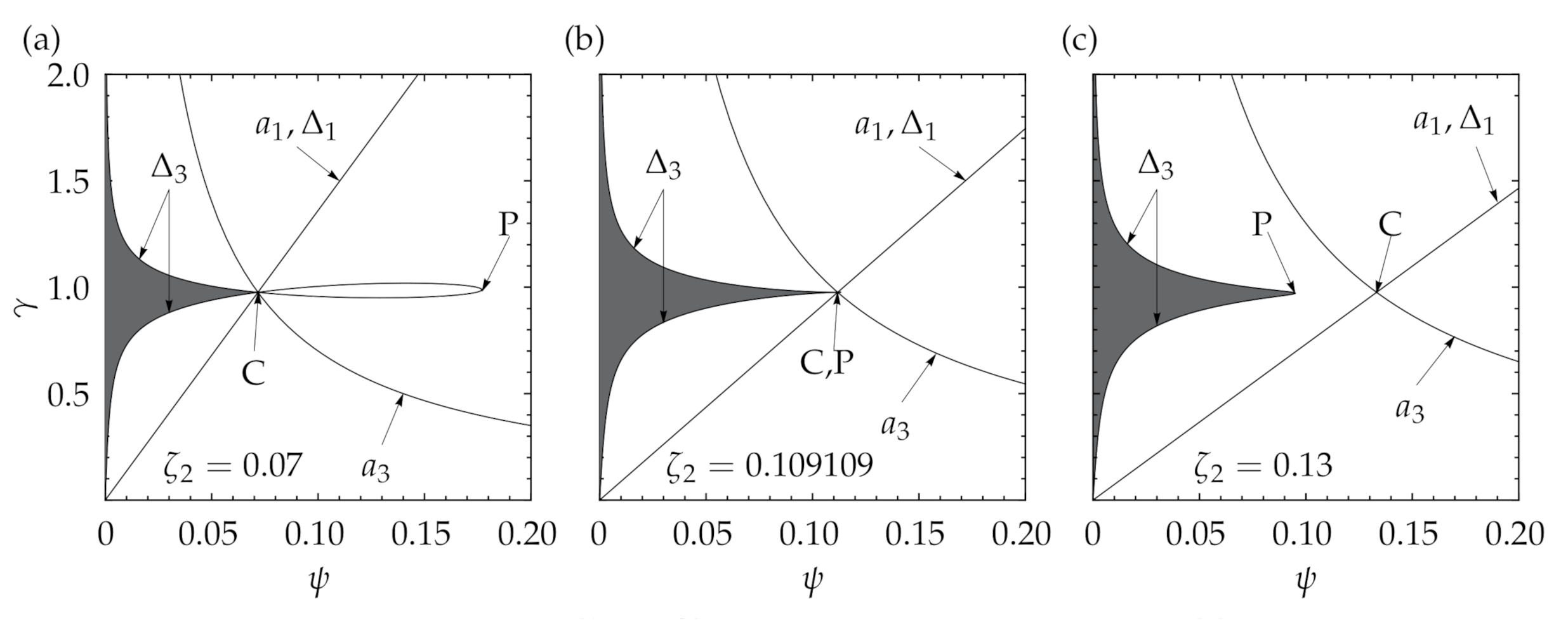
has only one couple of eigenvalues with positive real part, except in the loop delimited by Points C and P, where all four eigenvalues have positive real part. This scenario corresponds to a Hopf–Hopf (or double Hopf) bifurcation. In the following, the case of a single Hopf bifurcation is analyzed.
The first step of the analysis consists of transforming the system in Equation (9) into first-order form, similar to Equation (14), but including nonlinear terms up to the third order, which leads to
  z 1 z 2 z 3 z 4 = 0 0 1 0 0 0 0 1 1 γ 2 ε 2 ψ 2 ε ζ 2 γ 1 γ 2 ( ε + 1 ) 2 ψ 2 ( ε + 1 ) γ ζ 2 z 1 z 2 z 3 z 4 + 0 0 z 3 2 ( μ d μ s ) e v v 0 ( 3 v 0 + z 3 ) 6 v 0 3 ε k nl 2 z 2 3 z 3 2 ( μ d μ s ) e v v 0 ( 3 v 0 + z 3 ) 6 v 0 3 ( ε + 1 ) ε k nl 2 z 2 3     = A z + b   .
In the vicinity of the loss of stability, A has two couples of complex conjugate eigenvalues λ 1 , 2 = α 1 ± i ω 1 and λ 3 , 4 = α 2 ± i ω 2 . To decouple the linear part of the system, we define the transformation matrix
T = Re ( s 1 ) Im ( s 1 ) Re ( s 3 ) Im ( s 3 )   ,
where s 1 and s 3 are two of the eigenvectors of A , and we apply the transformation z = Ty , obtaining
y ˙ = T 1 Ay + T 1 b = Wy + b ˜   ,
where
W = α 1 ω 1 0 0 ω 1 α 1 0 0 0 0 α 2 ω 2 0 0 ω 2 α 2   .
For the sake of brevity, the explicit formulation of b ˜ is omitted here.
In the case of a single Hopf bifurcation, only α 1 becomes positive at the loss of stability, while α 2 remains negative. Therefore, only the first two equations of Equation (47) are linearly related to the bifurcation, while y 3 and y 4 have minor local effect at the bifurcation. Next, we aim at reducing the dynamics of the system to the so-called center manifold, which is a two-dimensional surface tangent at the bifurcation point to the subspace spanned by the two eigenvectors s 1 and s 2 related to the bifurcation. To do so, we approximate y 3 and y 4 by y 3 = η 320 y 1 2 + η 311 y 1 y 2 + η 302 y 2 2 and y 4 = η 420 y 1 2 + η 411 y 1 y 2 + η 402 y 2 2 , reducing the system to
  y 1 = α 1 y 1 + ω 1 y 2 + j + k = 2 , 3 a j k y 1 j y 2 k + h . o . t .   y 2 = ω 1 y 1 + α 1 y 2 + j + k = 2 , 3 b j k y 1 j y 2 k + h . o . t .   ,
where j and k are non-negative integers (more details on this procedure can be found in [26]) and h.o.t. stands for higher order terms.
The system in Equation (49) has the same form as Equation (39); therefore, exactly the same steps can be performed to reduce the system to its normal form, that is
r = α 1 ( v ) r + δ r 3   ,
where [26]
δ = 1 8 ( 1 ω 1 ( ( a 20 + a 02 ) ( a 11 + b 20 b 02 ) + ( b 20 + b 02 ) ( a 20 a 02 + b 11 ) ) + ( 3 a 30 + a 12 + b 21 + 3 b 03 ) ) .
Imposing ε = 0.05 , γ = γ opt and ζ 2 = 1.05   ζ 2 opt , we obtain
δ = 0.00474 + 0.68   k nl 2   .
Proceeding as done for the host system without DVA, we have that the non-trivial solutions of Equation (50) is given by
r = r * = α 1 * ( v v cr ) δ   ,
where α 1 * = d α 1 / d v | v = v cr . We notice that δ is positive if the DVA is linear ( k nl 2 = 0 ), which means that also in this case the bifurcation is subcritical, and it generates unstable periodic solutions. Analyzing other values of ζ 2 and ε 
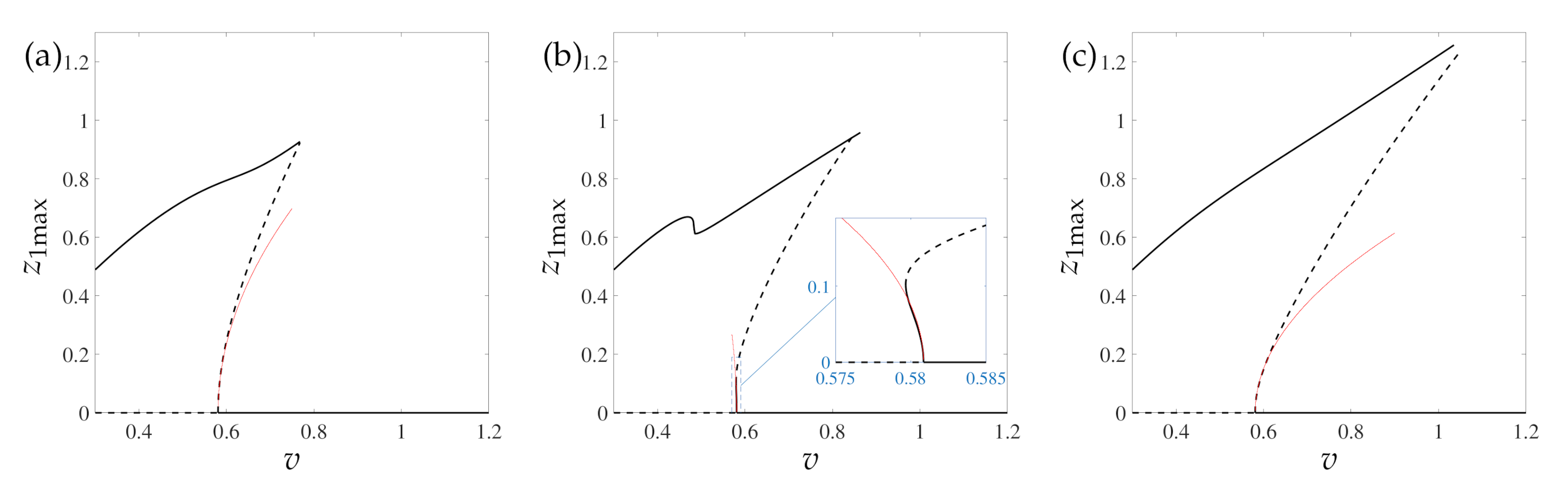
, we verified that the subcritical characteristic persists for a relatively large parameter value range. The corresponding bifurcation diagram is illustrated in 
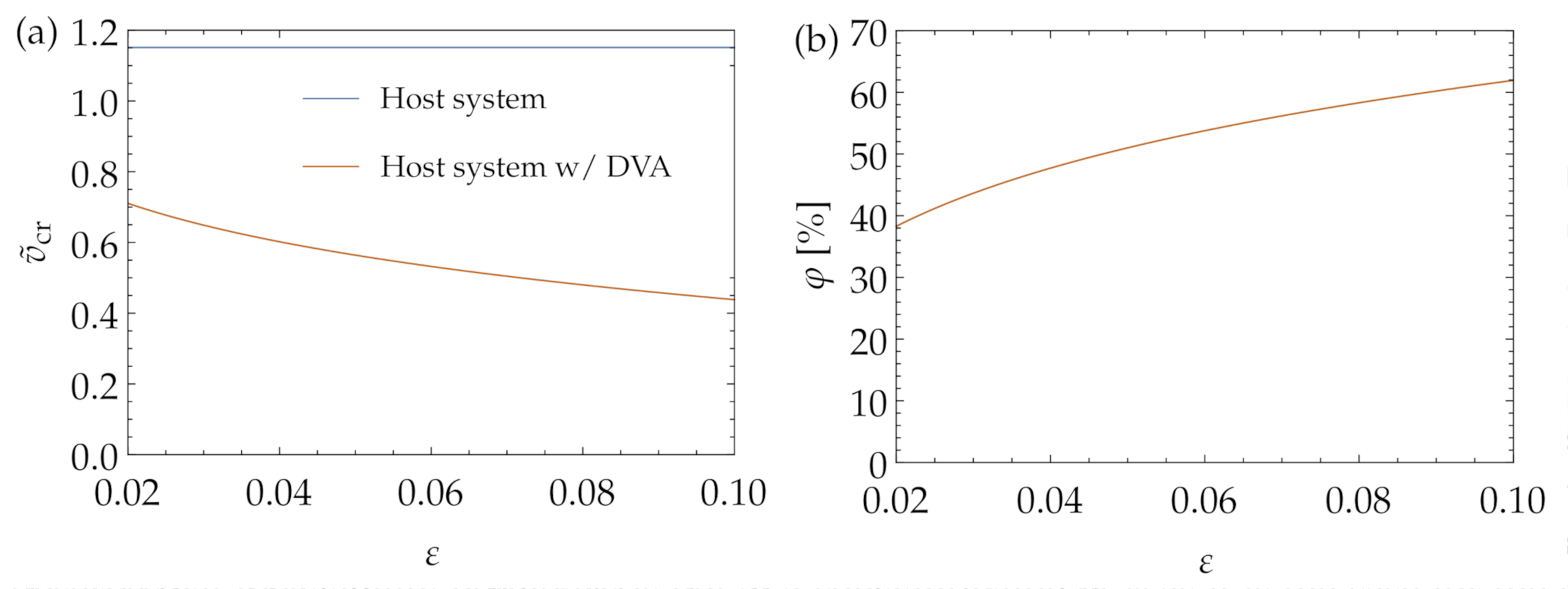
Figure 9a. Comparing Figure 9a and Figure 8a, we notice that, although the linear DVA does not change the characteristic of the bifurcation, the advantages in terms of vibrations suppression persist also in the nonlinear range. In fact, for the considered parameter values, in the host system without DVA, stick–slip oscillations exist for v 0 ,   1.83 , while, with the addition of the absorber, they are limited to the range v 0 ,   0.768 .
Equation (52) suggests that, if k nl 2 < 0.00697 , δ becomes negative, making therefore the bifurcation supercritical. This scenario is confirmed by the bifurcation diagram depicted in Figure 9b, for k nl 2 = 0.01 . Although at first sight it seems that the bifurcation is subcritical, the inset illustrates that the bifurcation is indeed supercritical; however, the branch of periodic solutions bends rapidly to the right in correspondence of a fold bifurcation, making the overall scenario similar to the case of k nl 2 = 0 . The figure confirms the correctness of the analytical computation; nevertheless, it also points out that the performed local analysis is unable to capture the global behavior of the system, which is not qualitatively affected by the variation of the nonlinear characteristic of the DVA’s spring. Furthermore, we notice that the addition of the softening nonlinear spring enlarges the bistable range, making stick–slip oscillations exist up to v < 0.86 , instead of 0.768 as in the case of k nl 2 = 0 .
Figure 9c illustrates the bifurcation diagram obtained for a hardening absorber’s spring ( k nl 2 = 0.01 ). In this case, the range of existence of stick–slip oscillations is further enlarged, persisting up to v < 1.035 . We also remark that increasing the value of k nl 2 above 0.01 or decreasing it below −0.01 provided only worse performance than those illustrated in Figure 9. This result suggests that any low order nonlinearity of the absorber’s stiffness is detrimental concerning the DVA effectiveness. This finding is somehow surprising, considering that in similar applications the addition of a properly tuned nonlinear term in the DVA’s stiffness provided some advantages [20,25,27].
Regarding Figure 9b, we notice that the branch of stick–slip oscillations presents two folds for v 0.48 . However, an analysis of the system’s steady state solutions before and after the folds did not reveal any particular detail relevant from an engineering point of view; therefore, the phenomenon was not analyzed in further detail. We also remark that, in Figure 9b,c, the branches of stable and unstable solutions do not encounter each other at a well defined point, as happens in Figure 8a, for instance. This is probably related to the fact that the branches of unstable solutions in Figure 9 were obtained adopting the shooting method (employing MatCont [28], a MATLAB-based toolbox for numerical continuation) of the system smoothed assuming that v rel is always positive. This assumption makes the considered system unable to exhibit stick–slip oscillations, but keeps it equivalent to the original system for v > z 3 . In contrast, the stable branches were obtained from direct numerical simulations of the full system. Therefore, inaccuracies of the smoothed system in the proximity of the onset of stick–slip motions are possible.
As mentioned at the beginning of this section, for ζ 2 < ζ 2 opt and γ = γ opt , the system undergoes a Hopf–Hopf bifurcation. However, acknowledging the fact that the bifurcation analysis seems to be an inefficient tool for investigating the post-bifurcation behavior of the system, which is dominated by large amplitude oscillations, and considering that the analysis of such a bifurcation requires a significant analytical effort, the detailed investigation of this case is omitted in this study.

6. Conclusions

In this study, the problem of suppressing FIVs through a DVA was addressed. Possibly the simplest system exhibiting FIVs was considered, i.e., the mass-on-moving-belt system, to which a classical DVA was attached. The optimal tuning of the absorber parameters was defined through an analytical procedure, which enabled us to reduce the critical velocity by approximately 50%, with an additional mass of only 5% of the primary system’s mass.
The post-bifurcation behavior analysis illustrated that, although a linear DVA is unable to change the bifurcation character at the loss of stability, it can still significantly reduce the extent of the bistable region. Globally, the area of existence of stick–slip oscillations is reduced by 58%, with a DVA mass of only 5%. The bifurcation analysis proved that it is possible to change the bifurcation character if a small softening term is included in the absorber. However, this has only a local beneficial effect, while, globally, it enlarges the region of existence of stick–slip motions. The performance also worsens if an additional hardening term is introduced, suggesting that the spring characteristic should be maintained as linear as possible. Large order nonlinearities, such as non-smoothness, might have beneficial effects; nevertheless, their analysis was not addressed in this study, and it is left for future developments. Other possible future developments of the present study include the analysis of the Hopf–Hopf bifurcation occurring at the loss of stability for ζ 2 < ζ 2 opt and the analysis of the performance of the DVA if the primary system has two DoF, encompassing, therefore, coupling instabilities as well [22].

Author Contributions

Conceptualization, G.H.; Data curation, J.L.H. and G.H.; Formal analysis, J.L.H. and G.H.; Funding acquisition, G.H.; Investigation, J.L.H. and G.H.; Methodology, J.L.H. and G.H.; Resources, G.H.; Software, J.L.H. and G.H.; Supervision, G.H.; Validation, J.L.H. and G.H.; Visualization, J.L.H. and G.H.; Writing—original draft, J.L.H. and G.H.; and Writing—review and editing, J.L.H. and G.H. All authors have read and agreed to the published version of the manuscript.

Funding

This research was funded by Hungarian National Science Foundation under grant number OTKA 134496 and by the NRDI Fund (TKP2020 IES, Grant No. BME-IE-NAT, and TKP2020 NC, Grant No. BME-NC) based on the charter of bolster issued by the NRDI Office under the auspices of the Ministry for Innovation and Technology.

Conflicts of Interest

The authors declare no conflict of interest.

References

  1. Papangelo, A.; Ciavarella, M.; Hoffmann, N. Subcritical bifurcation in a self-excited single-degree-of-freedom system with velocity weakening–strengthening friction law: Analytical results and comparison with experiments. Nonlinear Dyn. 2017, 90, 2037–2046. [Google Scholar] [CrossRef] [Green Version]
  2. Brockley, C.; Ko, P.L. Quasi-harmonic friction-induced vibration. J. Tribol. 1970, 92, 550–556. [Google Scholar] [CrossRef] [Green Version]
  3. Ibrahim, R. Friction-induced vibration, chatter, squeal, and chaos—part II: Dynamics and modeling. Appl. Mech. Rev. 1994, 47, 227–253. [Google Scholar] [CrossRef]
  4. Leine, R.; Van Campen, D.; De Kraker, A.; Van Den Steen, L. Stick-slip vibrations induced by alternate friction models. Nonlinear Dyn. 1998, 16, 41–54. [Google Scholar] [CrossRef]
  5. Hinrichs, N.; Oestreich, M.; Popp, K. On the modelling of friction oscillators. J. Sound Vib. 1998, 216, 435–459. [Google Scholar] [CrossRef]
  6. Kinkaid, N.; O’Reilly, O.M.; Papadopoulos, P. Automotive disc brake squeal. J. Sound Vib. 2003, 267, 105–166. [Google Scholar] [CrossRef]
  7. Ruina, A. Slip instability and state variable friction laws. J. Geophys. Res. Solid Earth 1983, 88, 10359–10370. [Google Scholar] [CrossRef]
  8. Dieterich, J.H. Modeling of rock friction: 1. Experimental results and constitutive equations. J. Geophys. Res. Solid Earth 1979, 84, 2161–2168. [Google Scholar] [CrossRef]
  9. Halderman, J.D.; Mitchell, C.D. Automotive Brake Systems; Prentice Hall: Upper Saddle River, NJ, USA, 1996. [Google Scholar]
  10. Brooks, P.; Crolla, D.; Lang, A.; Schafer, D. Eigenvalue Sensitivity Analysis Applied to Disc Brake Squeal. In Proceedings of the Institution of Mechanical Engineering, Braking of Road Vehicles, London, UK, 23–24 March 1993. [Google Scholar]
  11. Dunlap, K.B.; Riehle, M.A.; Longhouse, R.E. An investigative overview of automotive disc brake noise. SAE Trans. 1999, 515–522. [Google Scholar] [CrossRef]
  12. Cunefare, K.A.; Graf, A.J. Disc Brake Rotor Squeal Suppression Using Dither Control; Technical report, SAE Technical Paper; SAE International: Warrendale, PA, USA, 2001. [Google Scholar] [CrossRef]
  13. Papangelo, A.; Ciavarella, M. Effect of normal load variation on the frictional behavior of a simple Coulomb frictional oscillator. J. Sound Vib. 2015, 348, 282–293. [Google Scholar] [CrossRef]
  14. Den Hartog, J.P. Mechanical Vibrations; Courier Corporation: North Chelmsford, MA, USA, 1985. [Google Scholar]
  15. Casalotti, A.; Arena, A.; Lacarbonara, W. Mitigation of post-flutter oscillations in suspension bridges by hysteretic tuned mass dampers. Eng. Struct. 2014, 69, 62–71. [Google Scholar] [CrossRef]
  16. Verstraelen, E.; Habib, G.; Kerschen, G.; Dimitriadis, G. Experimental passive flutter suppression using a linear tuned vibration absorber. AIAA J. 2017, 55, 1707–1722. [Google Scholar] [CrossRef]
  17. Frahm, H. Means for Damping the Rolling Motion of Ships. U.S. Patent 970,368, 13 September 1910. [Google Scholar]
  18. Hamouda, M.N.H.; Pierce, G.A. Helicopter vibration suppression using simple pendulum absorbers on the rotor blade. J. Am. Helicopter Soc. 1984, 29, 19–29. [Google Scholar] [CrossRef] [Green Version]
  19. Sims, N.D. Vibration absorbers for chatter suppression: A new analytical tuning methodology. J. Sound Vib. 2007, 301, 592–607. [Google Scholar] [CrossRef] [Green Version]
  20. Habib, G.; Kerschen, G.; Stepan, G. Chatter mitigation using the nonlinear tuned vibration absorber. Int. J. Non-Linear Mech. 2017, 91, 103–112. [Google Scholar] [CrossRef] [Green Version]
  21. Popp, K.; Rudolph, M. Vibration control to avoid stick-slip motion. J. Vib. Control 2004, 10, 1585–1600. [Google Scholar] [CrossRef]
  22. Chatterjee, S. On the design criteria of dynamic vibration absorbers for controlling friction-induced oscillations. J. Vib. Control 2008, 14, 397–415. [Google Scholar] [CrossRef]
  23. Niknam, A.; Farhang, K. On the passive control of friction-induced instability due to mode coupling. J. Dyn. Syst. Meas. Control 2019, 141. [Google Scholar] [CrossRef]
  24. Gantmakher, F.R. Lectures in Analytical Mechanics; Mir: Moscow, Russia, 1970. [Google Scholar]
  25. Habib, G.; Kerschen, G. Suppression of limit cycle oscillations using the nonlinear tuned vibration absorber. Proc. R. Soc. Math. Phys. Eng. Sci. 2015, 471, 20140976. [Google Scholar] [CrossRef] [PubMed] [Green Version]
  26. Kuznetsov, Y.A. Elements of Applied Bifurcation Theory; Springer Science & Business Media: Berlin, Germany, 2013; Volume 112. [Google Scholar]
  27. Malher, A.; Touzé, C.; Doaré, O.; Habib, G.; Kerschen, G. Flutter control of a two-degrees-of-freedom airfoil using a nonlinear tuned vibration absorber. J. Comput. Nonlinear Dyn. 2017, 12. [Google Scholar] [CrossRef]
  28. Dhooge, A.; Govaerts, W.; Kuznetsov, Y.A.; Meijer, H.G.E.; Sautois, B. New features of the software MatCont for bifurcation analysis of dynamical systems. Math. Comput. Model. Dyn. Syst. 2008, 14, 147–175. [Google Scholar] [CrossRef]
Figure 1. (a) The host system without absorber; and (b) free body diagram of the host system.
Lubricants 08 00100 g001
Figure 2. The host system with the attached DVA.
Lubricants 08 00100 g002
Figure 3. The weakening friction law with μ s = 1 , μ d = 0.5 , v 0 = 0.5 .
Lubricants 08 00100 g003
Figure 4. Stability diagrams for different values of ζ 2 and ε = 0.05 : (a) ζ 2 = 0.07 ; (b) ζ 2 = 1 / 2 ε / ( 1 + ε ) = 0.109109 ; and (c) ζ 2 = 0.13 .
Lubricants 08 00100 g004
Figure 5. Vanishing loop of the Δ 3 = 0 curve. The blue line was obtained utilizing the optimal damping as defined by the analytical procedure ζ 2 = ζ 2 opt , the green line corresponds to the optimal solution obtained by the numerical procedure and the yellow and red lines are obtained for ζ 2 values slightly larger and smaller, respectively, than ζ 2 opt .
Lubricants 08 00100 g005
Figure 6. Comparison of host system with and without DVA with varying ζ 1 , other parameters as in Table 3: (a) critical velocities; and (b) improvement curve.
Lubricants 08 00100 g006
Figure 7. Comparison of host system with and without DVA with varying ε : (a) critical velocities; and (b) improvement curve.
Lubricants 08 00100 g007
Figure 8. (a) Bifurcation diagram for the host system without DVA; the thin red line marks analytical solutions, black lines numerical ones and dashed lines the numerical unstable solutions. (b) Steady state solutions of the system for v = 1.3 ; solid line is the stable solution and dashed line is the unstable solution. (c) Time series of the system leading to the steady state solutions represented in (b) with initial conditions z h = ( 1.367 ,   0 ) T (blue line) and z h = ( 1.36 ,   0 ) T (red line). Other parameter values are as in Table 3.
Lubricants 08 00100 g008
Figure 9. Bifurcation diagrams for the host system with the DVA for parameter values as in Table 3, γ = γ opt and ζ 2 = ζ 2 opt : (a) k nl 2 = 0 , (b) k nl 2 = 0.01 ; and (c) k nl 2 = 0.01 . Solid lines are stable solutions, dashed lines are unstable solutions and thin red lines are analytical solutions.
Lubricants 08 00100 g009
Table 1. Parameter grid for the optimum search.
ParameterminmaxStep
ζ 2 0.10.11 10 5
γ 0.975890.97591 10 6
ψ 0.11240.1126 10 5
Table 2. Comparison of numerical and analytical results.
ParameterNumericalAnalyticalRelative Error [%]
ζ 2 0.109770.1091090.605867 [%]
γ 0.9758990.9759000.000109945 [%]
ψ 0.112470.1118030.596226 [%]
v cr 1.366781.368830.364409 [%]
Table 3. Numerical input data.
μ s μ d v 0 ε ζ 1
10.50.50.050.05
Publisher’s Note: MDPI stays neutral with regard to jurisdictional claims in published maps and institutional affiliations.

