A Computational Fluid Dynamics Study on Shearing Mechanisms in Thermal Elastohydrodynamic Line Contacts

Abstract

A computational fluid dynamics (CFD) model of the thermal elastohydrodynamically lubricated (EHL) line contact problem has been developed for the purpose of exploring the physical processes that occur inside a thin EHL film subjected to shearing motion. The Navier–Stokes equations are solved by using the finite volume method (FVM) in a commercial CFD software, ANSYS Fluent. A set of user-defined functions (UDF) are used for computing viscosity, density, heat source, temperature of moving surfaces and elastic deformation of the top roller according to well-established equations commonly used in the EHL theory. The cavitation problem is solved by taking into account multiphase mixture flow. The model combinations of Houpert and Ree–Eyring and of Tait and Carreau were used for modeling the non-Newtonian behavior of Squalane and the results were compared. Both rheological models suggest the existence of shear-band and plug-flow at high fluid pressure. Due to the differences in viscosity at GPa-level pressure, the chosen model has substantial influence on the computed shear stress and temperature distributions in the high-pressure region. This shows the importance of using correct rheology information in the whole range of pressure, temperature, and shear strain rate.

1. Introduction

Lubricated machine elements designed for transferring high loads and high rotational speeds mainly operate in the elastohydrodynamic lubrication (EHL) regime. In a typical hard EHL contact, parts in relative motion are separated by a highly pressurized thin lubricant film. High pressure inside the film is generated due to a converging gap that is formed by the moving surfaces, operating conditions and lubricant properties. In such films, fluid pressure ranges from about 0.5 to 3 GPa. As a consequence of the high fluid pressure, lubricant viscosity increases several orders of magnitude, and the lubricant can reach a quasi-solid state. The tremendous increase in viscosity has a couple of implications. Firstly, being highly viscous helps the lubricant to stay in the contact zone and to separate the contacting surfaces. The quasi-solid lubricant film acts as a wedge between two moving surfaces and forces them to deform elastically. Secondly, by increasing viscosity more heat is generated in the film. The amount of generated heat becomes even larger when sliding is increased. As a result of the high heat, viscosity and consequently shear stress decreases. All these factors contribute to the friction in such contacts [1,2,3] and understanding its causes is one of the major current issues in the industry.

In experimental studies of EHL two main approaches are commonly encountered [4]. The first approach focuses on measuring EHL quantities by using well-controlled instruments (e.g., ball-on-disc and twin-disc tribometer) that replicate the type of contact in a machine element that is being studied. The second approach is based on shearing a highly pressurized fluid sample at high strain rates by using specially designed rheometers, capable of reaching high pressure levels. Over the years, researchers working in both fields have generated a significant amount of knowledge about EHL. In general, both sides agree on the effects of operating conditions and material properties on EHL film thickness. However, there is still an ongoing debate on rheological model that best describes the physical behavior of EHL films. In many cases, researchers dealing with EHL friction measurements use a Ree–Eyring based model [4] to describe their experimental data. On the other hand, researchers dealing with high pressure rheometry are advocating a Carreau based model [4]. Several articles that heated up the debate were published in 2014 and 2015 by Spikes and Jie [4,5], Bair and his co-authors [6], and it seems that there is still no consensus on this topic.

It should be acknowledged that besides the two main approaches described above, another experimental approach for studying EHL contacts has been developed. In 1989, Cann and Spikes [7] proposed a method based on measuring the temperature inside the contact and extracting the viscosity and shear stress based on the Carslaw–Jaeger model. In the following years, several papers dealing with the proposed method were published [8,9].

When it comes to numerical modeling of EHL, the most common approach is based on solving the Reynolds equation, which is derived from the Navier–Stokes equations by making assumptions that proved to be valid for the studies of thin fluid films. The two most important assumptions are that the thickness of the film is much smaller than its length and that fluid pressure is constant in gap height direction. As being very accurate, the Reynolds equation represents a standard equation in numerical modeling of EHL. However, the development of the computing power in the last decades has enabled a few researchers to obtain a full solution of EHL based on the Navier–Stokes equations.

In 2002, Almqvist and Larsson [10] performed the first thermal CFD simulation of EHL. They modeled Newtonian fluid behavior by using Roelands viscosity equation. They found that the decreasing effect of temperature on viscosity results in better numerical stability and they were able to reach a pressure of approximately 0.7 GPa but with a significant computational cost. In 2004, the same group of authors performed CFD analysis of EHL on the surface roughness scale while using Roelands and Ree–Eyring equations for viscosity modeling [11]. They discovered that the Ree–Eyring model leads to a more stable numerical solution due to having a decreasing effect on viscosity and a suppressing effect on the singularity in the momentum equation. In 2008, Hartinger et al. [12] found that their CFD solution of thermal EHL is in good agreement with the generalized Reynolds solution, for non-Newtonian fluid behavior and pressure of about 0.6 GPa. The authors relied on the Roelands viscosity model modified by Houpert and on the Ree–Eyring rheological model. In 2016, Lohner et al. [13] used commercial multiphysics software to develop a model of the EHL line contact problem based on the generalized Reynolds equation. They have also used the Ree–Eyring model and found that their results are in good correlation with previously published CFD results with pressures of up to approximately 0.6 GPa. In 2017, Hajishafiee et al. [14] performed a CFD analysis of thermal EHL and reached higher pressure levels over 3 GPa. They computed viscosity by using the model combination of Houpert and Ree–Eyring. For achieving numerical stability at high pressure, the authors assumed physically unrealistic elastic behavior of steel parts with reduced Young’s modulus up to approximately 690 GPa. They concluded that high computational expense of CFD technique is justifiable in cases when assumptions in the Reynolds equation are not applicable.

What is common for all the introduced CFD studies of EHL is that they all rely on the Roelands/Houpert and Ree–Eyring viscosity and rheology models. However, in many theoretical and experimental studies of EHL the model combination of Tait and Carreau is also widely used. Furthermore, the former CFD studies also reveal that the Reynolds approach might not be sufficient when the assumptions in the Reynolds equation are not applicable. As the aim is to study the physical processes inside a thin EHL film subjected to shearing motion under high load for different rheological behaviors, the CFD approach is used in order to not be misled due to the assumptions of the Reynolds approach. Additionally, differences in results for the model combinations of Houpert and Ree–Eyring and of Tait and Carreau will be presented and as it will be shown, the differences are substantial.

2. Methods

In the first part of this section, governing equations of fluid dynamics are presented. The second part of the section describes the equations from the field of EHL. In the last part of the section, fluid domain geometry and the used numerical methods are presented.

2.1. Governing Equations

Fluids in motion are described by the equations of conservation of mass and momentum. To include thermal effects, the equation of conservation of energy was coupled together with the former two. For a multiphase flow and the mixture model, the governing equations read as follows [15].

The conservation of mass equation [15], widely known as a continuity equation, reads

$$\frac{\partial }{\partial t}\left({\rho }_m\right)+\nabla ·\left({\rho }_m {\overrightarrow{\mathsf{\nu }}}_{\mathrm{m}}\right)=0,$$

(1)

where ${\rho }_m$ is the mixture density and ${\overrightarrow{\mathsf{\nu }}}_{\mathrm{m}}$ is the mass-averaged velocity, that read

$${\rho }_m={\displaystyle \sum }_{k=1}^n{\alpha }_k{\rho }_k,$$

(2)

$${\overrightarrow{\mathsf{\nu }}}_{\mathrm{m}}=\frac{{\sum }_{k=1}^n{\alpha }_k{\rho }_k{\overrightarrow{\mathsf{\nu }}}_{\mathrm{k}}}{{\rho }_m}.$$

(3)

When gravitational and body force are neglected, the conservation of momentum equation [15], commonly known as the Navier–Stokes equation, reads as follows

$$\frac{\partial }{\partial t}\left({\rho }_m{\overrightarrow{\mathsf{\nu }}}_{\mathrm{m}}\right)+\nabla ·\left({\rho }_m{\overrightarrow{\mathsf{\nu }}}_{\mathrm{m}}{\overrightarrow{\mathsf{\nu }}}_{\mathrm{m}}\right)=-\nabla p+\nabla ·\left(\stackrel{=}{\tau }\right)+\nabla ·\left({\displaystyle \sum }_{k=1}^n{\alpha }_k{\rho }_k{\overrightarrow{\mathsf{\nu }}}_{\mathrm{dr},\mathrm{k}}{\overrightarrow{\mathsf{\nu }}}_{\mathrm{dr},\mathrm{k}}\right),$$

(4)

where $\stackrel{=}{\tau }$ is the stress tensor and ${\overrightarrow{\mathsf{\nu }}}_{\mathrm{dr},\mathrm{k}}$ is the drift velocity for secondary phase k, that read

$$\tau ={\mu }_m\left(\nabla {\overrightarrow{\mathsf{\nu }}}_{\mathrm{m}}+\nabla {\overrightarrow{\mathsf{\nu }}}_{\mathrm{m}}{}^{\mathrm{T}}\right),$$

(5)

$${\overrightarrow{\mathsf{\nu }}}_{\mathrm{dr},\mathrm{k}}={\overrightarrow{\mathsf{\nu }}}_{\mathrm{k}}-{\overrightarrow{\mathsf{\nu }}}_{\mathrm{m}}.$$

(6)

In Equation (5), ${\mu }_m$ represents viscosity of the mixture described by the following expression

$${\mu }_m={\displaystyle \sum }_{k=1}^n{\alpha }_k{\mu }_k.$$

(7)

The conservation of energy equation [15] reads

$$\frac{\partial }{\partial t}{\displaystyle \sum }_{k=1}^n\left({\alpha }_k{\rho }_k{E}_k\right)+\nabla ·{\displaystyle \sum }_{k=1}^n\left({\alpha }_k{\overrightarrow{\mathsf{\nu }}}_{\mathrm{k}}\left({\rho }_k{E}_k+p\right)\right)=\nabla ·\left(k_{eff}\nabla \mathrm{T}\right)+S_T,$$

(8)

where $S_T$ is the heat source term that for EHL conditions takes into account heat generated in the lubricant film by the viscous heating ($Q_{s\mathrm{hear}h}$) and by the compression work ($-W$) [16] as follows

$$S_T=Q_{s\mathrm{hear}}-W,$$

(9)

$$Q_{s\mathrm{hear}}=\mu \left(\nabla \overrightarrow{\mathsf{\nu }} :\nabla \overrightarrow{\mathsf{\nu }}+\nabla \overrightarrow{\mathsf{\nu }}:{\left(\nabla \overrightarrow{\mathsf{\nu }}\right)}^T-\frac{2}{3}{\left(\nabla ·\overrightarrow{\mathsf{\nu }}\right)}^2\right).$$

(10)

2.2. Cavitation Modeling

When modeling thin lubricating films, one must resolve the cavitation problem that occurs at the outlet of the contact zone, at the position where the two contacting surfaces are starting to diverge from each other. As a consequence of cavitation, negative pressure occurs, which must be avoided when computing fluid force (integral of fluid pressure) in the force-balance equation that reads [16]

$$w={{\displaystyle \int }}_{x_{inlet}}^{x_{outlet}}pdx.$$

(11)

The cavitation problem was solved by using the “full cavitation model” by Singhal et al. [17] that can be used if a fluid is modeled as a mixture of liquid and vapor phases. According to this model, fluid density $\rho$ and vapor volume fraction $\alpha$ are a function of the vapor mass fraction $f$ as follows

$$\frac{1}{\rho }=\frac{f}{{\rho }_v}+\frac{1-f}{{\rho }_l},$$

(12)

$$\alpha \equiv f\frac{\rho }{{\rho }_v}.$$

(13)

where indices $v$ and $l$ denote vapor and liquid phase, respectively. Vapor mass fraction $f$ was obtained from the solution of the transport equation coupled together with the continuity and the Navier–Stokes equations, as follows

$$\frac{\partial }{\partial t}\left(\rho f\right)+\nabla ·\left(\rho \overrightarrow{\mathrm{v}}f\right)=\nabla ·\left(\mathsf{\Gamma }\nabla f\right)+R_e-R_c.$$

(14)

Here, terms $R_e$ and $R_c$ denote vapor generation and condensation rates, respectively, which are dependent on the vapor pressure [15,17] as follows

$$if p\le p_{vap}, R_e=0.02\frac{\sqrt{k}}{\sigma }{\rho }_l{\rho }_v{\left[\frac{2}{3}\frac{p_v-p}{{\rho }_l}\right]}^{1/2}\left(1-f_v-f_g\right),$$

(15)

$$if p>p_{vap}, R_c=0.01\frac{\sqrt{k}}{\sigma }{\rho }_l{\rho }_v{\left[\frac{2}{3}\frac{p-p_v}{\rho }\right]}^{1/2}{f}_v,$$

(16)

As recommended by Hartinger et al. [12], a vapor pressure of 5000 Pa was used in the present study.

2.3. Lubricant Properties

For modeling EHL conditions, user-defined functions (UDFs) were used for computing density, viscosity, heat source (Equation (9)), temperature profile of the moving surfaces and elastic deformation of the top roller. The UDFs were written in computer language C.

2.3.1. Density Equations

Commonly, lubricant density in isothermal conditions is computed according to the Dowson–Higginson expression [18] that reads

$$\rho \left(p,T\right)= {\rho }_0\left(1+\frac{A p}{1+B p}\right),$$

(17)

where $A=0.6·{10}^{-9} {\mathrm{m}}^2/\mathrm{N}$ and $B=1.7·{10}^{-9} {\mathrm{m}}^2/\mathrm{N}$. For modeling thermal effects, Bos [19] included a linear temperature dependence in the Dowson–Higginson equation, as follows

$$\rho \left(p,T\right)= {\rho }_0\left(1+\frac{A p}{1+B p}\right)\left[1-\epsilon \left(T-T_R\right)\right].$$

(18)

Due to being more physically relevant, Habchi [20] recommends using a density equation that is derived from the Tait equation of state, that reads

$$\rho \left(p,T\right)= {\rho }_0\left(\frac{1}{V_0/V_R}\times \frac{1}{V/V_0}\right).$$

(19)

The disadvantage of the equations that rely on the Tait equation of state is that they require specific fluid data which are not easily found in the literature. The effect of pressure on density was included in Equation (19) by using a modified version of the Tait equation of state for the volume relative to the volume at ambient pressure $V_0$, as follows [21]

$$\frac{V}{V_0}=1-\frac{1}{1+K_0^{\prime }}ln\left[1+\frac{p}{K_0}\left(1+K_0^{\prime }\right)\right],$$

(20)

where $K_0$ is the isothermal bulk modulus at zero pressure that reads

$$K_0=K_{00}exp\left(-{\beta }_{K}T\right),$$

(21)

The temperature effect on density was included in Equation (19) by using volume at ambient pressure relative to the ambient pressure volume at the reference temperature $V_R$, as follows [21]

$$\frac{V_0}{V_R}=1+a_V\left(T-T_R\right).$$

(22)

2.3.2. Viscosity Equations for Newtonian Fluid Behavior

For the Newtonian fluid behavior and isothermal conditions, viscosity was computed according to the Roelands formula [22] that reads

$${\eta }_R\left(p\right)={\mu }_0 exp\left\{\left[ln\left({\mu }_0\right)+9.67\right]\left[-1+{\left(1+5.1\times {10}^{-9}p\right)}^Z\right]\right\},$$

(23)

where $Z$ is Roelands pressure–viscosity index that can be computed by using pressure–viscosity coefficient $\alpha$, as follows

$$Z=\frac{\alpha }{5.1·{10}^{-9}\left(ln\left({\mu }_0\right)+9.67\right)}.$$

(24)

When thermal effects are taken into account, viscosity can be computed according to the Houpert (modified Roelands) [23] formula as follows

$${\eta }_H\left(p,T\right)={\eta }_R exp\left(-{\beta }^{*}\left(T-T_R\right)\right),$$

(25)

where

$${\eta }_R\left(p,T\right)={\mu }_0 exp\left\{\left[ln\left({\mu }_0\right)+9.67\right]\left[-1+{\left(1+5.1 \times {10}^{-9} p\right)}^Z{\left(\frac{T-138}{T_R-138}\right)}^{-S_0}\right]\right\},$$

(26)

$$S_0=\frac{\beta \left(T_r-138\right)}{ln\left({\mu }_0\right)+9.67} ,$$

(27)

$${\beta }^{*}=\left(ln\left({\mu }_0\right)+9.67\right){\left(1+5.1\times {10}^{-9}p\right)}^Z \frac{S_0}{T_R-138}.$$

(28)

2.3.3. Rheological Models

For modeling non-Newtonian fluid behavior two rheological models are used, the Ree–Eyring and the Carreau. The Ree–Eyring model reads [24]

$${\eta }_{Ree-Eyring}\left(p,T, \dot{\gamma }\right)=\frac{{\tau }_0}{\dot{\gamma }}sin{h}^{-1}\left(\frac{{\eta }_0\dot{\gamma }}{{\tau }_0}\right),$$

(29)

where ${\tau }_0$ is the Eyring stress that denotes the threshold where the Newtonian fluid behavior ends and the non-Newtonian fluid behavior starts. To avoid division by zero, instead of ${\eta }_0$ in Equation (29) Hartinger [25] suggests using the Houpert equation (Equation (25)). In addition, to avoid numerical error during simulation, Hartinger also recommends using the Ree–Eyring model only if strain rate is larger than an arbitrarily chosen minimum value of $\dot{\gamma }=1\times {10}^{-8} {\mathrm{s}}^{-1}$, otherwise he suggests using Houpert equation [25]. This can be written in the following fashion

$$\eta \left(T,P,\dot{\gamma }\right)=\left\{\begin{array}{ccc}{\eta }_H& for& \dot{\gamma }<{\dot{\gamma }}_{min}\\ \frac{{\tau }_0}{\dot{\gamma }}sin{h}^{-1}\left(\frac{{\eta }_H\dot{\gamma }}{{\tau }_0}\right)& for& \dot{\gamma }\ge {\dot{\gamma }}_{min}\end{array}\right\}.$$

(30)

According to Björling et al. [21], the Carreau equation for the non-Newtonian viscosity reads

$${\eta }_{Carreau}\left(p,T, \dot{\gamma }\right)=\mu {\left(1+{\left(\dot{\gamma }{\lambda }_R\frac{\mu }{{\mu }_R}\frac{T_R}{T}\frac{V}{V_R}\right)}^2\right)}^{\left(n-1\right)/2},$$

(31)

where $\mu$ is the limiting low-shear viscosity that is described by the Vogel-like formula

$$\mu ={\mu }_{\infty }exp\left(\frac{B_F{\phi }_{\infty }}{\phi -{\phi }_{\infty }}\right).$$

(32)

Here, $\phi$ represents the dimensionless viscosity scaling parameter that reads [21]

$$\phi =\left(\frac{T}{T_R}\right){\left(\frac{V}{V_R}\right)}^g.$$

(33)

It should be mentioned that the model combination of Tait and Carreau does not incorporate limiting shear stress behavior of liquids [21], unlike the model combination of Houpert and Ree–Eyring in which temperature effect mimics this phenomenon. To overcome this drawback of the model combination of Tait and Carreau, Björling et al. [21] suggests truncating shear stress if the limiting value of shear stress is reached, which is defined as follows

$${\tau }_L=\mathsf{\Lambda }\mathrm{p},$$

(34)

where $\mathsf{\Lambda }$ parameter is derived from experiments.

2.4. Surface Temperature

Surface temperature, evaluated at location $x$ and caused by heat flux $q_f$ acting at location $\widehat{x}$, was computed according to Carslaw–Jaeger thermal boundary condition that for 1D line contact reads [24]

$$T_{CJ}\left(x\right)=\sqrt{\frac{1}{\pi ·{\rho }_s·C_s·k_s·u_s}}·{{\displaystyle \int }}_{-\infty }^x{q}_f\left(\widehat{x}\right)\frac{d\widehat{x}}{\sqrt{x-\widehat{x}}} .$$

(35)

where index $s$ denotes the solid part.

However, Equation (35) has the limit of applicability depending on the Peclet number that can be calculated by using formula [24]

$$Pe=\frac{L·u_s}{\frac{k_s}{{\rho }_s{C}_s}},$$

(36)

where $L$ represents a characteristic length scale. For EHL contacts, the characteristic length scale is the Hertzian half width $b$. Finally, in order to use Equation (35), it is recommended that the Peclet number is larger than 5 [24]. In 2018, Hartinger [25] showed that for the EHL line contact problem, surface temperatures predicted by Carslaw–Jaeger equation closely matched experimental measurements.

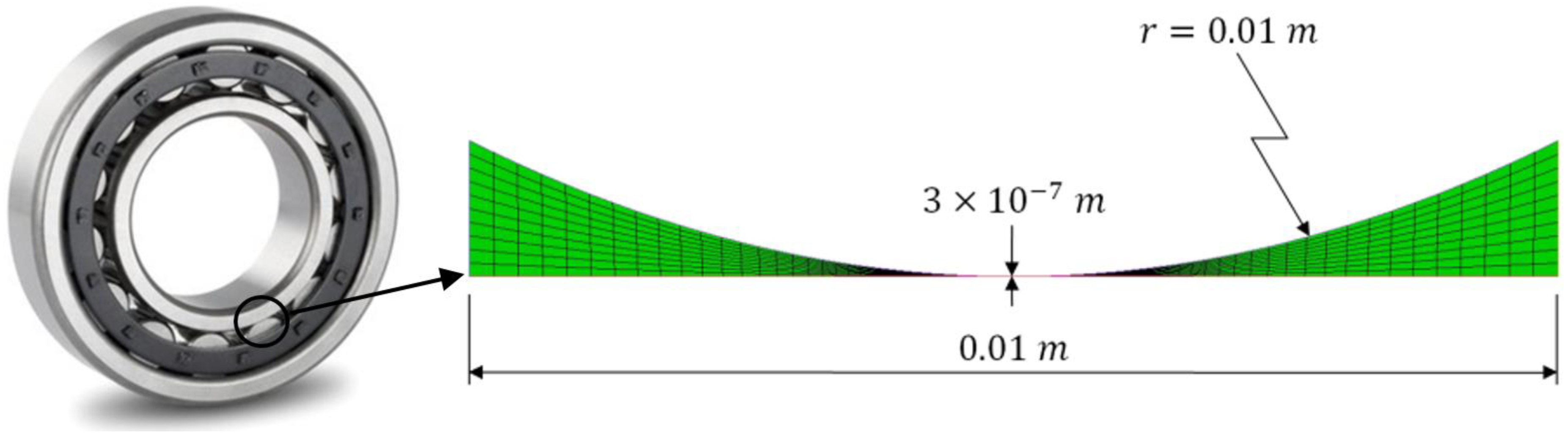
2.5. The Film Thickness Equation

The elastic deformation of the top roller, evaluated at the location $x$ and caused by the pressure $p$ acting at location $\widehat{x}$, is modeled by using the film thickness equation that reads [16]

$$h\left(x\right)=h_0+\frac{x^2}{2R^{\prime }}-\frac{2}{\pi E^{\prime }}{{\displaystyle \int }}_{-\infty }^{\infty }p\left(\widehat{x} \right)ln\left({\left|x-\widehat{x}\right|}^2\right)d\widehat{x},$$

(37)

where $E^{\prime }$ is the reduced elastic modulus and $R^{\prime }$ is the reduced contact radius that read as follows

$$E^{\prime }=2·{\left(\left(1-{\upsilon }_1^2\right)/E_1+\left(1-{\upsilon }_2^2\right)/E_2\right)}^{-1},$$

(38)

$$R^{\prime }=1/R_1+1/R_2.$$

(39)

2.6. Mesh Generation and Numerical Method

The EHL line contact is common in many machine elements, such as spur gears or cylindrical roller bearings. The 2D fluid domain geometry shown in Figure 1 was found to be appropriate for solving this kind of problem, since in this type of contact the pressure distribution in the third dimension is uniform. The geometry consists of a roller on a flat surface. Although a bottom flat surface was used instead of a curved surface, the effect of the bottom curvature was taken into account in computing deformation of the top roller through reduced radius of curvature $R^{\prime }$ (Equation (39)). The reduced geometry was chosen for the purpose of direct comparison of the obtained results against the results of Srirattayawong [16] who used similar geometry and the same CFD software. ANSYS SpaceClaim was used for creation of the CAD model and high-quality mesh was generated in ANSYS ICEM CFD.

Figure 1. The 2D fluid domain of the elastohydrodynamic lubrication (EHL) line contact problem.

The equations of mass conservation, momentum and energy were solved in ANSYS Fluent that was based on the FVM. FVM approximates the solution of the non-linear partial differential equations on discrete places on mesh geometry which are termed cells. Cell refers to a small surface (2D) or volume (3D) surrounding each mesh point. In order to obtain a solution at each cell center, flux values at the cell edges were used. In this way, the properties of the equations coming from the conservation laws (mass, momentum, energy) were mirrored, where the change of a quantity in the cell center was only due to fluxes across the cell edges.

The UDFs, based on the equations presented in the first part of this section, were dynamically loaded with the Fluent solver. The UDFs for density, viscosity and heat source were updated in each iteration while the UDFs for surface temperature and elastic deformation of the top roller were updated at the beginning of each time step. The film thickness equation was implemented in the UDF for dynamic mesh. It was coupled with the force-balance equation (Equation (11)) in such way that the parameter ${\mathrm{h}}_0$ was corrected at the beginning of each time step until the forces are balanced. As recommended by Srirattayawong [16], motion of the mesh nodes in the interior of the fluid domain was controlled by using spring-based smoothing method.

A pressure-based solver was employed for solving the conservation equations in a sequential and iterative manner [16]. In addition, the chosen algorithm for pressure–velocity coupling was PISO [16]. When it comes to spatial discretization, the Green–Gauss node-based method was chosen for resolving gradients [16]. When using a multiphase mixture flow model, PRESTO pressure interpolation scheme is recommended. For other quantities that are a product of the conservation equations, second-order upwind scheme was used, except for vapor, where only first-order upwind method was available. Finally, for solving time derivatives, second-order implicit method was used.

3. Results and Discussion

In the first part of the section, the results of the mesh verification test are presented, which prove that the results of the CFD model are independent of the mesh resolution. In the second part of the section, the results for the isothermal conditions are given. In the third part of the section, the thermal results at the pressure of about 1.0 GPa are presented by using Squalane as a lubricant and the model combinations of Houpert and Ree–Eyring and of Tait and Carreau for computing viscosity.

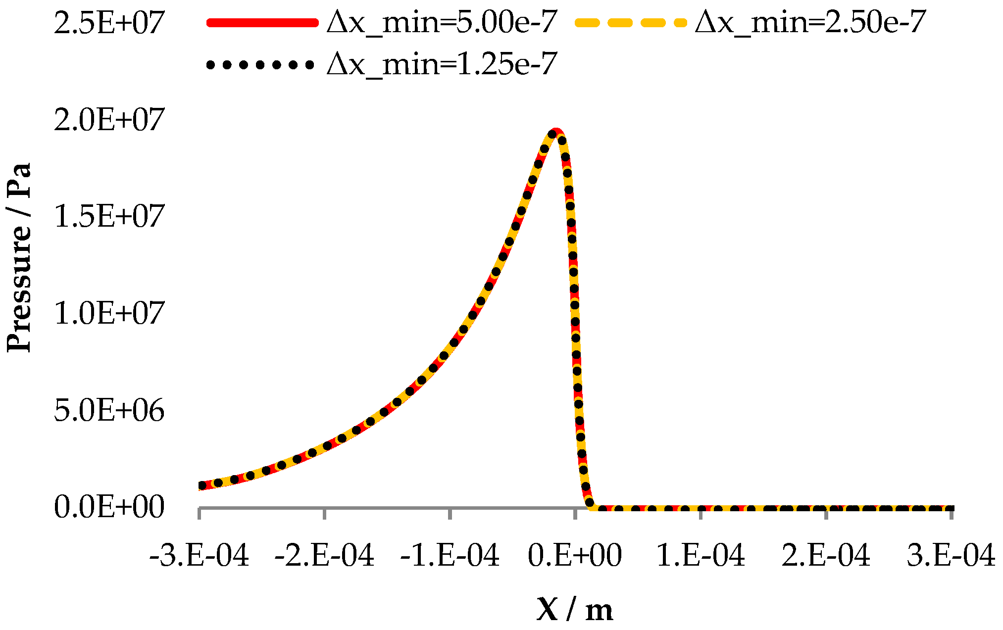
3.1. Mesh Verification Test

Solving the EHL problem by using a CFD approach based on the Navier–Stokes equations is computationally very expensive. In addition to a fine mesh, complex physics and a large number of very complex UDFs slow down the computation. In order to speed up the computation, the CFD model was modified for a parallel run on eight cores by using an Intel(R) Xeon(R) E5-2697 v3 CPU. It was found that an even larger number of cores cause communication overhead that can again slow down the computation, therefore eight cores were deemed to be an optimum.

In gap height direction, 10 cells are used [16]. In the horizontal direction, a finer mesh is used in the central region of the fluid domain where higher pressure is generated and all the processes of interest take place. Three mesh resolutions of the central region are tested, as shown in Figure 2 and Table 1.

Figure 2. Pressure distribution after solving cavitation problem for the three mesh resolutions.

Table 1. Mesh verification test.

Min. Cell Size of in X-dir.	Total no. of Cells	Max. Pressure in Pa	CPU Time in s
$\Delta {\mathrm{x}}_{\min }=5.00\times {10}^{-7}$ m	13,480	$1.941\times {10}^7$	304
$\Delta {\mathrm{x}}_{\min }=2.50\times {10}^{-7}$ m	25,480	$1.943\times {10}^7$	370
$\Delta {\mathrm{x}}_{\min }=1.25\times {10}^{-7}$ m	49,480	$1.943\times {10}^7$	496

Results presented in Table 1 show that the difference in maximum pressure between the coarsest and the finest mesh resolutions is only 0.02 MPa. The case with the finest mesh had 63% longer CPU time than the case with the coarsest mesh. For the purpose of saving time, the small difference in the results was found acceptable, and thus the coarsest mesh resolution shown in Table 1 was used for obtaining all results presented in this article.

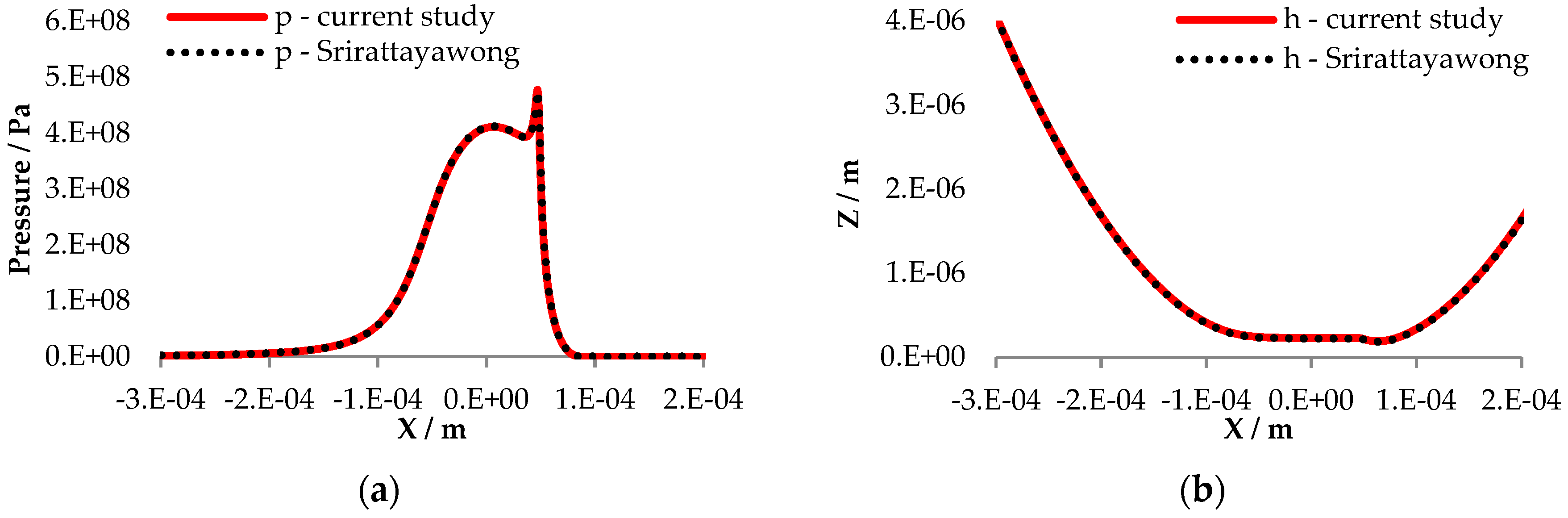
3.2. Isothermal Conditions, Newtonain Fluid Behavior, Low Pressure

Input parameters including operating conditions and properties of the considered steel as solid and oil as lubricant are given in Table 2. Dowson–Higginson (Equation (17)) and Roelands (Equation (23)) equations are used for modeling the effect of pressure on density and viscosity, respectively.

Table 2. Input parameters.

Parameter	Value		Unit
Operating conditions
External load, $w$	$50$		$\mathrm{kN}/\mathrm{m}$
Entrainment speed, $u_{ent}$	$2.5$		$\mathrm{m}/\mathrm{s}$
Reference temperature, $T_R$	$313.15$		$\mathrm{K}$
Reduced radius of curvature, $R^{\prime }$	$0.01$		$\mathrm{m}$
Properties of solids
	steel [16]	ceramics [16]
Modulus of elasticity, $E$	$210$	$450$	$\mathrm{GPa}$
Poisson ratio, $\upsilon$	$0.3$	$0.15$	-
Density, $\rho$	$7850$	$3800$	$\mathrm{kg}/{\mathrm{m}}^3$
Specific heat capacity, $C$	$460$	$1050$	$\mathrm{J}/\left(\mathrm{kgK}\right)$
Thermal conductivity, $k$	$47$	$29$	$\mathrm{W}/\left(\mathrm{mK}\right)$
Properties of liquids
	oil [16]	Squalane
Dynamic viscosity at ambient pressure and $T_R$, ${\mu }_0$	$0.01$	$0.0156$ [21]	$\mathrm{P}\mathrm{a} \mathrm{s}$
Density, $\rho$	$850$	$794.6$ [26]	$\mathrm{kg}/{\mathrm{m}}^3$
Dynamic viscosity of vapor phase, ${\mu }_v$	$8.97\times {10}^{-6}$	$8.97\times {10}^{-6}$1	$\mathrm{Pa} \mathrm{s}$
Density of vapor phase, ${\rho }_v$	$0.0288$	$0.0288$1	$\mathrm{kg}/{\mathrm{m}}^3$
Specific heat capacity, $C$	-	$2104$ [26]	$\mathrm{J}/\left(\mathrm{kgK}\right)$
Thermal conductivity, $k$	-	$0.21$ [27] 2	$\mathrm{W}/\left(\mathrm{mK}\right)$
Thermal expansivity, $\epsilon$	-	$8.36\times {10}^{-4}$ [21]	${\mathrm{K}}^{-1}$
Houpert and Ree–Eyring input parameters
	oil [16]	Squalane
Temperature–viscosity coefficient, $\beta$	-	$0.038$ [28]	${\mathrm{K}}^{-1}$
Eyring stress, ${\tau }_0$	-	$3.0\times {10}^6$ [29] 3	$\mathrm{Pa}$
Roelands pressure–viscosity index, $Z$	0.689	$0.6442$4	-
Tait and Carreau input parameters
		Squalane [21]
Pressure rate of change of isothermal bulk modulus at $p=0$, $K_0^{\prime }$		$11.74$	-
Thermal expansivity defined for volume linear with $T$, $a_V$		$8.36\times {10}^{-4}$	${\mathrm{K}}^{-1}$
$K_0$ at zero absolute temperature, $K_{00}$		$8.658\times {10}^9$	$\mathrm{Pa}$
Temperature coefficient of $K_0$, ${\beta }_K$		$6.332\times {10}^{-3}$	${\mathrm{K}}^{-1}$
Thermodynamic interaction parameter, $g$		$3.921$	-
Viscosity scaling parameter for unbounded viscosity, ${\phi }_{\infty }$		$0.1743$	-
Fragility parameter in the new viscosity equation, $B_F$		$24.50$	-
Viscosity extrapolated to infinite temperature, ${\mu }_{\infty }$		$0.9506\times {10}^{-4}$	$\mathrm{Pa} \mathrm{s}$
Relaxation time at $T_R$ and ambient pressure, ${\lambda }_R$		$2.26\times {10}^{-9}$	$\mathrm{s}$
Power law exponent, $n$		$0.463$	-
Limiting stress pressure coefficient, $\mathsf{\Lambda }$		$0.075$	-

¹ Vapor phase parameters for Squalane are assumed to be the same as for oil. ² Thermal conductivity is taken from the referenced paper by taking an average value from the thermal conductivity vs. pressure graph. ³ Eyring stress is derived from the shear stress vs. strain rate graph from the referenced paper. ⁴ Roelands pressure–viscosity index is calculated by using Equation (24) and pressure–viscosity coefficient of $\alpha =18.1 {\mathrm{GPa}}^{-1}$ [30].

The pressure distribution curve shown in Figure 3a is characterized by the pressure spike near the outlet of the contact zone. Another typical EHL feature is the minimum film thickness at the outlet of the contact zone which can be seen in the film thickness distribution curve (Figure 3b). These results are in good agreement with the results reported by Srirattayawong [16] who reported a maximum pressure of 0.474 GPa and minimum film thickness of 0.1869 μm for the lowest mesh resolution he considered. In the present study, for approximately the same mesh resolution, the maximum pressure is 0.477 GPa and the minimum film thickness is 0.191 μm. The small difference in the obtained results can be assigned to a small difference in mesh or a possible different value of vapor pressure, which was not reported in the referenced study.

Figure 3. Comparison of the isothermal results for slide-to-roll ratio (SRR) = 0 against the results presented by Srirattayawong [16]. (a) Pressure distribution; (b) film thickness distribution.

Contour plots for the isothermal conditions are given in Figure 4.

Figure 4. Contour plots for isothermal conditions and SRR = 0. (a) Static pressure; (b) velocity streamlines; (c) density; (d) viscosity; (e) strain rate; (f) shear stress; (g) oil volume fraction; (h) vapor volume fraction.

The pressure contours (Figure 4a) show that pressure varies only in the gap length direction while the pressure variation in the gap height direction is not present or it is insignificantly small. The velocity streamlines in Figure 4b show that the moving surfaces drag lubricant particles through the narrow passage between them. As the lubricant particles approach the outlet, due to pressure gradient and moving surfaces, their speed increases and they reach a maximum speed at the minimum film thickness location. Such speed increase is a necessary condition for maintaining continuity of the flow. In Figure 4c, a slight change of oil density in the high-pressure region can be noticed. Figure 4d shows that viscosity is uniformly distributed in gap height direction, which is expected since viscosity is only pressure dependent and pure rolling conditions are imposed. It is also expected to have maximum viscosity at the pressure spike location. Strain rate contours in Figure 4e show that the strain rate is increased in the regions where the localized slope of the velocity profile is the steepest. From shear stress contours shown in Figure 4f, it can be seen that the highest shear stress is in the regions where the lubricant is very viscous and strain rate is high, which is at the pressure spike location. Finally, on the basis of the oil and vapor volume fraction contours given in Figure 4g,h, we can clearly distinguish the regions where liquid and vapor phases are dominating the mixture flow. As expected, the vapor phase is dominant in the cavitation region at the outlet of the contact zone.

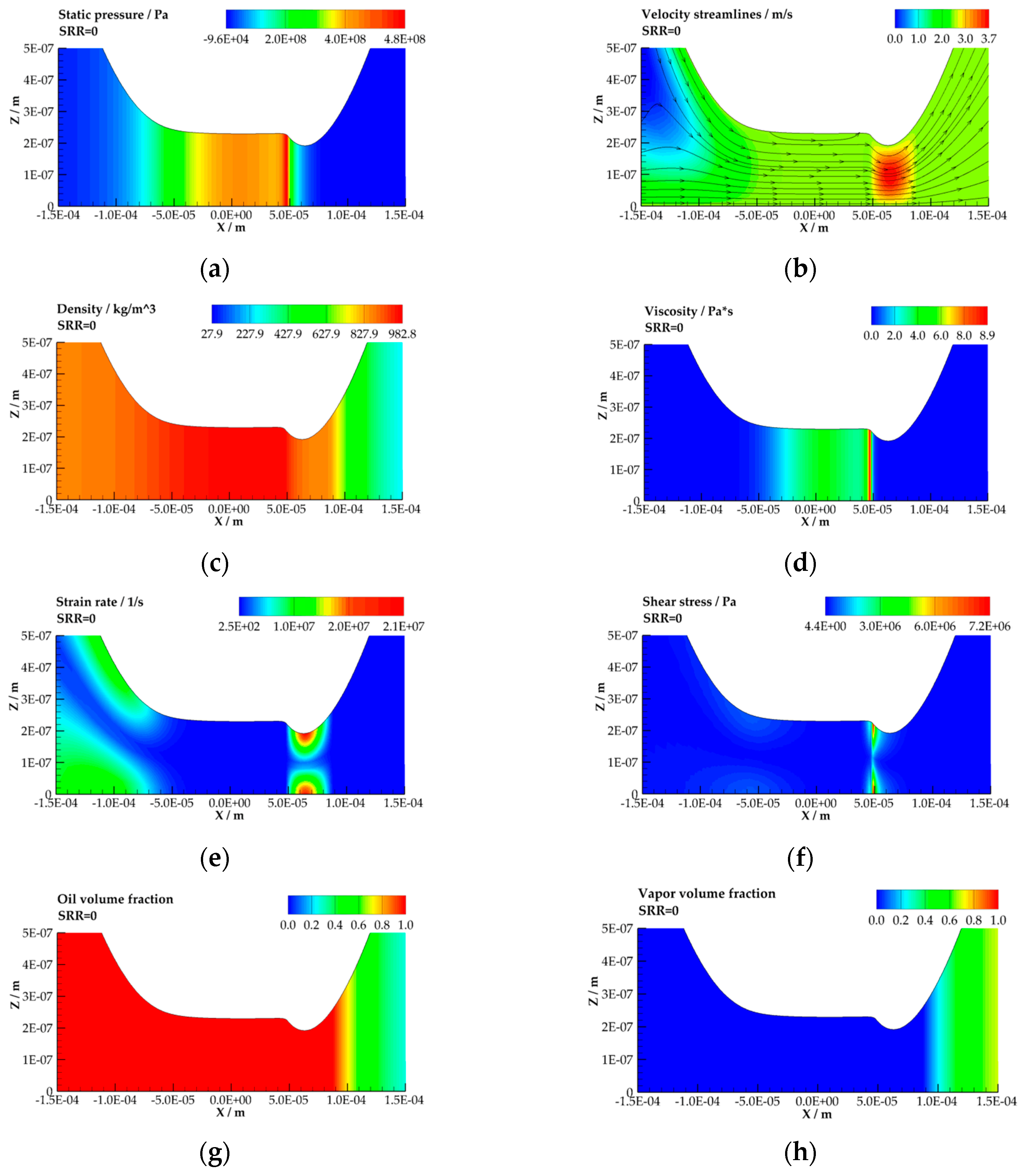
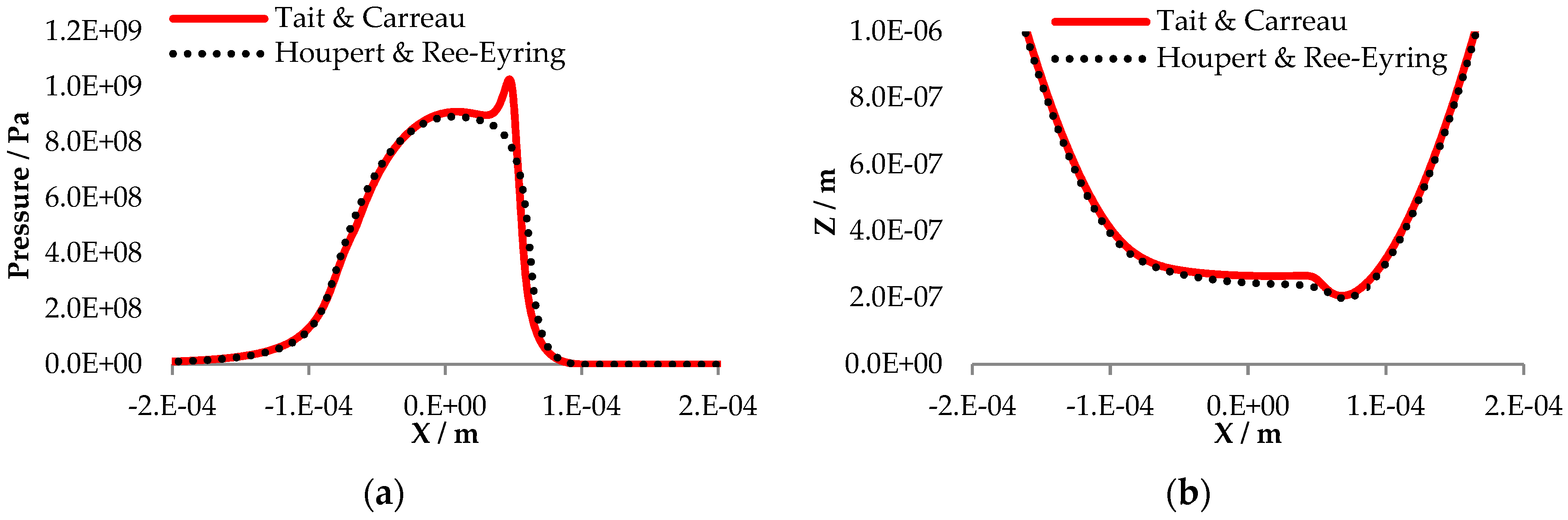
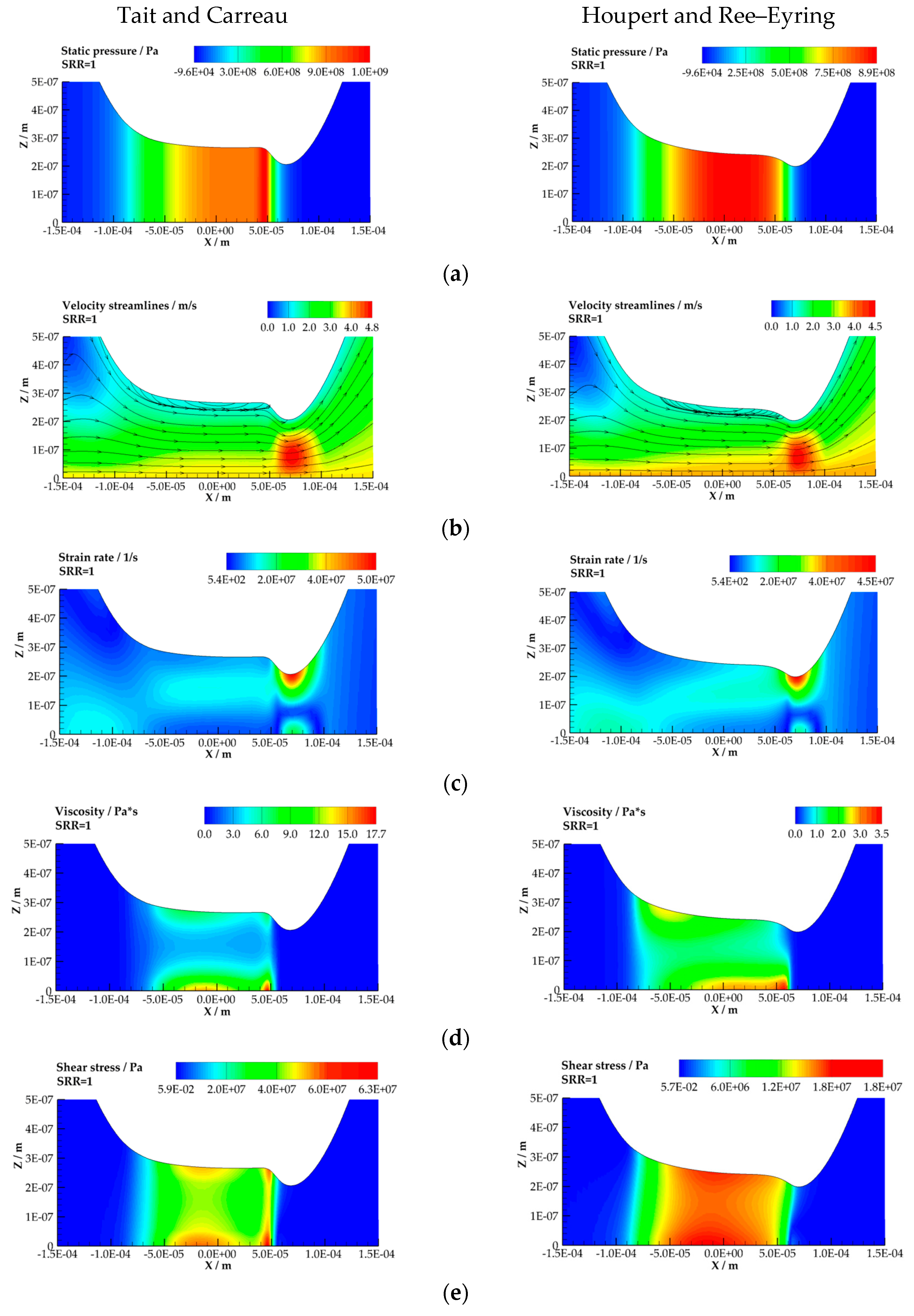
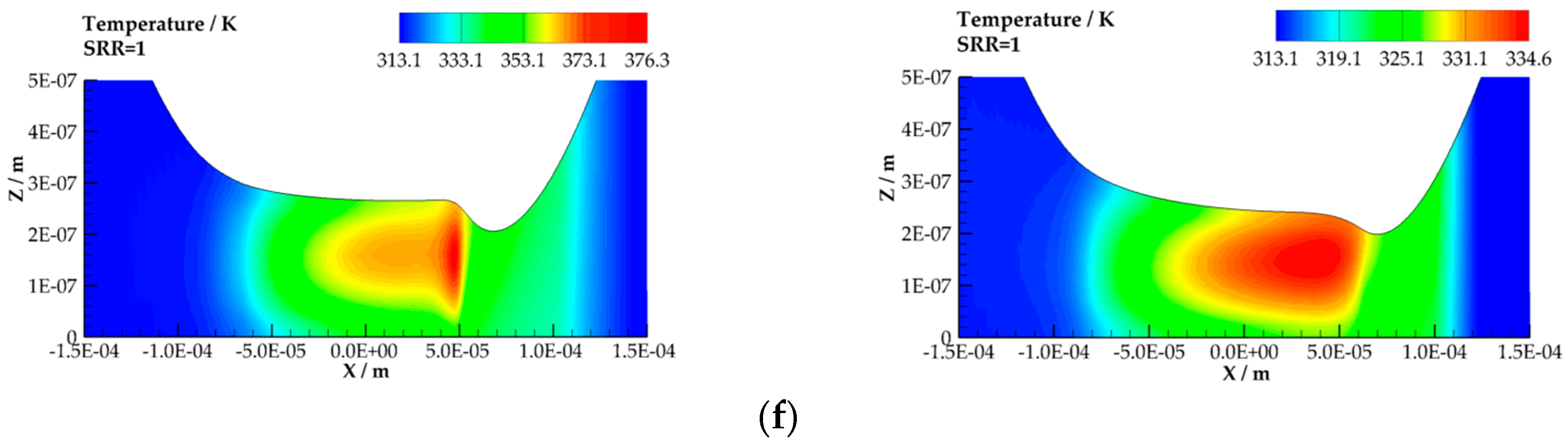
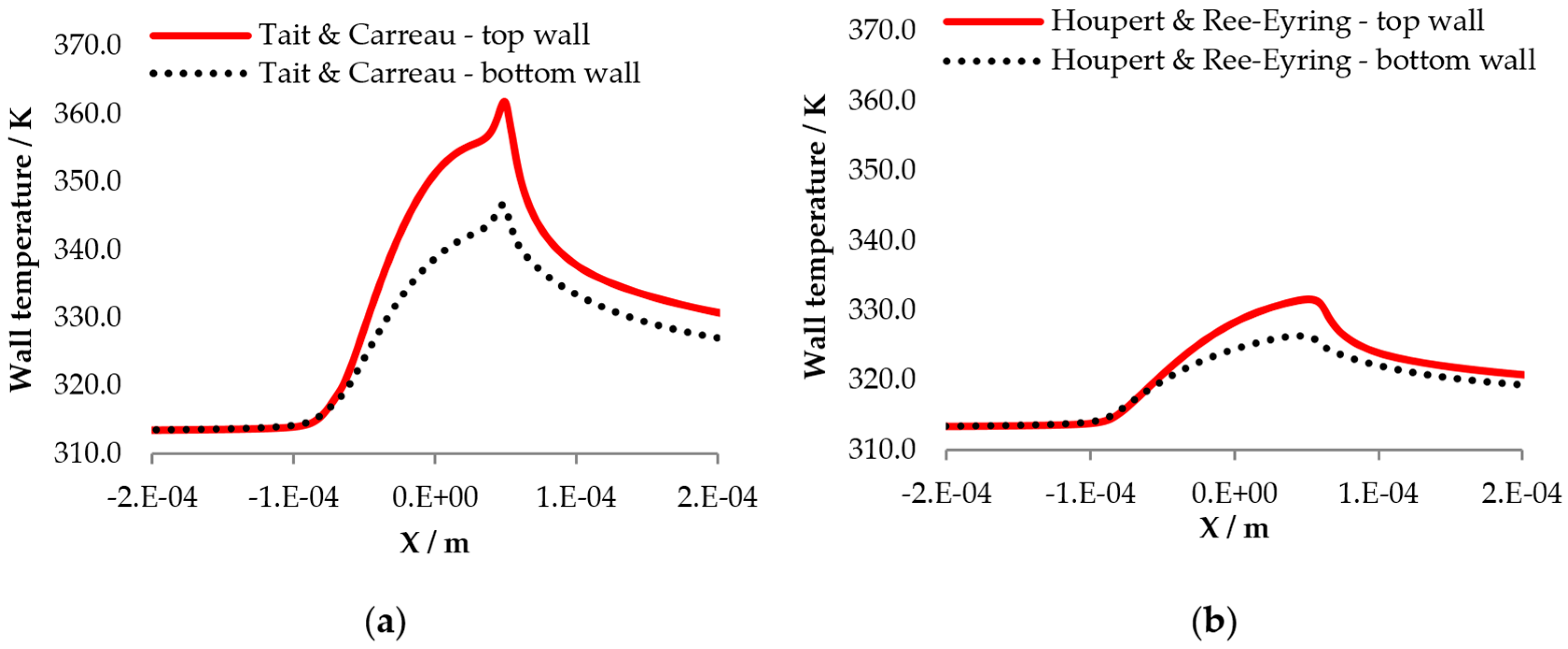
3.3. Thermal Conditions, Non-Newtonain Fluid Behavior, High Fluid Pressure

To reach higher fluid pressure for less computation time and better numerical stability, ceramics is used as material of the solid parts. Ceramics have more than two times higher Young’s modulus of elasticity than steel and thus suffer less elastic deformation under the same applied load. This brings benefit in numerical stability since solution becomes more stable as the solid wall deforms less. Squalane is used as lubricant since its properties for the model combinations of Houpert and Ree–Eyring and of Tait and Carreau can be derived from the available literature (see Table 2). A load of 120 kN is applied on the top roller. The speed of the bottom surface has been set to 3.75 m/s while the top surface rotates with 125 rad/s (1.25 m/s) which gives an entrainment speed of 2.5 m/s and a slide-to-roll ratio (SRR) of 1 (50% of sliding). The Pecklet number for the slower moving surface is 14, and 42 for the faster moving surface which means that the Carslaw–Jaeger thermal boundary condition is appropriate for this case.

The pressure and the film thickness results are presented in Figure 5.

Figure 5. Comparison of model combinations of Tait and Carreau and of Houpert and Ree–Eyring for thermal conditions and SRR = 1. (a) Pressure distribution; (b) film thickness distribution.

Figure 5a shows that the pressure distribution for the model combination of Houpert and Ree–Eyring is very smooth, while for the model combination of Tait and Carreau it is characterized by a very pronounced pressure spike. This implies that the effect of temperature and strain rate on fluid is much stronger in the case when the model combination of Houpert and Ree–Eyring is used. Note that it is not only the rheological behavior that is different for the two model combinations. The Newtonian viscosity behavior is also different, see Section 2.3. Different pressure distributions result in slightly different film thickness distributions, as Figure 5b shows. Namely, the higher fluid pressure in the case when the model combination of Tait and Carreau is used means that the lubricant opposes to the applied load with more force, which results in the less narrow passage between the contacting surfaces.

Contour plots for the two model combinations are presented in Figure 6. From the pressure contours given in Figure 6a, it can be seen that for the same operating conditions, the model combination of Tait and Carreau results in about 0.11 GPa higher maximal pressure. The velocity streamlines for both model combinations (Figure 6b) show that fluid particles in the vicinity of the slower moving top wall are stuck and do not flow easily. This phenomenon is known as a plug-flow and most probably, it will become even more pronounced at higher pressure.

Figure 6. Comparison of contour plots for model combinations of Tait and Carreau and of Houpert and Ree–Eyring for thermal conditions and SRR = 1. (a) Static pressure; (b) velocity streamlines; (c) strain rate; (d) viscosity; (e) shear stress; (f) temperature.

The strain rate contours presented in Figure 6c indicate the existence of a shear-band for both model combinations. Additionally, it can be noticed that the value of the maximum strain rate is higher for the model combination of Tait and Carreau. The viscosity contours in Figure 6d demonstrate that the shear-band is more pronounced when the model combination of Tait and Carreau is used, which can be assigned to the more viscous fluid, higher temperature and higher strain rate. Figure 6e shows that shear stress is much higher in the Tait and Carreau based case. This is the consequence of the more viscous lubricant and higher strain rate. The higher shear stress results in higher friction force and thus in higher friction. The coefficient of friction was 0.0405 in the Tait and Carreau based case and 0.0176 in the Houpert and Ree–Eyring based case.

When temperature contours (Figure 6f) for both model combinations are compared, it can be seen that the heat source is closer to the slower moving top wall. This is expected behavior since heat needs more time to penetrate into the faster moving bottom wall. The location of the heat source governs the location of the shear-band. As it can be noticed from Figure 6c, the shear-band is in both cases closer to the slower moving top wall. Additionally, Figure 6f shows that the model combination of Tait and Carreau gives significantly higher temperature in the region around the pressure spike location. The big difference in temperature at this particular location is due to the more viscous fluid which results in more viscous heating. Furthermore, warmer fluid at the central part of the contact zone results in warmer fluid at the outlet zone and thus a difference in temperature between the two model combinations can be seen in the cavitation zone. The difference in fluid temperatures causes a difference in wall temperatures. As Figure 7 shows, the walls are much hotter in the Tait and Carreau based case.

Figure 7. Comparison of the wall temperature for thermal conditions and SRR = 1. (a) model combination of Tait and Carreau; (b) model combination of Houpert and Ree–Eyring.

For the model combination of Tait and Carreau, the shear stress is truncated to the limiting shear stress defined by Equation (34). By dividing shear stress $\tau$ (Figure 6e, left) by limiting shear stress ${\tau }_L$ (Equation (34)), the contour plot presented in Figure 8 is obtained, which serves to show regions in the fluid domain where the limiting shear stress is reached. From the contact inlet to the beginning of the cavitation zone, the highest $\tau /{\tau }_L$ ratio is approximately 0.85, which means that the limiting shear stress has not be reached in this area. A $\tau /{\tau }_L$ ratio higher than 1 can be seen only in the cavitation zone where the pressure is close to zero or even negative. Since limiting shear stress has no physical meaning in the cavitation zone, it can be claimed that under given operating conditions, the limiting shear stress of Squalane has not been reached.

Figure 8. Contour plot of shear stress to limiting shear stress ratio (model combination of Tait and Carreau).

The change of the viscosity of Squalane with pressure, under zero strain rate and constant temperature (Newtonian behavior), is presented in Figure 9. The change of the viscosity of Squalane with strain rate, under constant pressure and constant temperature (non-Newtonian behavior), is shown in Figure 10. It should be mentioned that the results presented in these two figures were obtained without truncating shear stress to the limiting value, since Figure 8 shows that the limiting shear stress has not been reached in the CFD simulation based on the model combination of Tait and Carreau. Here, the viscosity is instead dominated by thermal softening.

Figure 9. The change of viscosity with pressure for zero strain rate and arbitrarily chosen constant values of temperature.

Figure 10. The change of viscosity with pressure at reference temperature (${\mathrm{T}}_{\mathrm{R}}=313.15 \mathrm{K}$) and arbitrarily chosen constant values of strain rate.

This is in agreement with the conclusion derived by Habchi et al. [31], who found that when operating conditions are such that the limiting shear stress is not reached, then truncating shear stress to the limiting value is of no importance for predicting friction.

As it can be seen from Figure 9, at zero strain rate and reference temperature of T = 313.15 K, there is only a slight difference in viscosity prediction between the model combinations Houpert and Ree–Eyring (H and R-E) and Tait and Carreau (T and C). However, if temperature is increased, it can be noticed that the difference in viscosity increases. At T = 353.15 K and p = 1.0 GPa the results differ by approximately one order of magnitude. This indicates that the temperature effect is mainly responsible for the difference in viscosity predictions by Tait and Houpert Newtonian viscosity models.

When the effect of strain rate on viscosity is taken into consideration (Figure 10), it can be noticed that at the lowest examined value of strain rate and pressure of up to approximately 0.2 GPa, there is only a small variation in viscosity between the two combination of models. However, at pressures above 0.2 GPa, the difference is becoming larger as pressure is increased, for the all three sets of conditions. At $\dot{\mathsf{\gamma }}$ = 5e7 1/s and p = 1.0 GPa the results differ by approximately one order of magnitude.

4. Conclusions

The presented results in this article demonstrate that the CFD technique can be successfully used in numerical modeling of the EHL line contact problem. The CFD approach has the advantage of not relying on assumptions as the Reynolds approach. One of the biggest disadvantages of the CFD approach is a high computational cost, which is directly caused by the low under-relaxation factors required to control the motion of the solid parts and pressure generation inside a lubricant.

The obtained solution for the isothermal conditions at low pressure of about 0.5 GPa was found to be in a very good agreement with the recent literature, which speaks in favor of the validity of the conducted numerical procedure.

The obtained results for the thermal conditions at high pressure of about 1 GPa show that the solution depends highly on the considered rheological model. This indicates that the choice of a rheological model and/or lubricant properties, at higher pressure levels, can cause significant deviation between numerical simulations and experimental measurements. This is in agreement with the recent study by Hartinger [25], who concluded that at the pressure of about 0.6 GPa, his CFD model of the EHL line contact problem overestimates shear-thinning effect on viscosity when compared to experimental measurements of friction and surface temperatures.

From this study it is not possible to say if one of the two considered model combinations is better than the other, but shows that it is of significant importance to correctly determine the effective viscosity at high pressure and high shear strain rates. Otherwise, the occurrence of shear-bands and the friction cannot be predicted correctly.

References

- Johnson, K.L.; Roberts, A.D. Observations of viscoelastic behaviour of an elastohydrodynamic lubricant film. Proceed. R. Soc. London A Math. Phys. Sci. 1974, 20, 217–242. [Google Scholar] [CrossRef]
- Tevaarwerk, J.L.; Johnson, K.L. The influence of Fluid Rheology on the Performance of Traction Drives. ASME J. Lubr. Tech. 1979, 101, 266–273. [Google Scholar] [CrossRef]
- Evans, C.R.; Johnson, K.L. The rheological properties of elastohydrodynamic lubricants. Proceed. Inst. Mech. Eng. C J. Mech. Eng. Sci. 1986, 200, 303–312. [Google Scholar] [CrossRef]
- Spikes, H.; Jie, Z. History, Origins and Prediction of Elastohydrodynamic Friction. Tribol. Lett. 2014, 56, 1–25. [Google Scholar] [CrossRef]
- Spikes, H.; Jie, Z. Reply to the Comment by Scott Bair, Philippe Vergne, Punit Kumar, Gerhard Poll, Ivan Krupka, Martin Hartl, Wassim Habchi, Roland Larson on “History, Origins and Prediction of Elastohydrodynamic Friction” by Spikes and Jie in Tribology Letters. Tribol. Lett. 2015, 58, 1–6. [Google Scholar] [CrossRef]
- Bair, S.; Vergne, P.; Kumar, P.; Poll, G.; Krupka, I.; Hartl, M.; Habchi, W.; Larsson, R. Comment on “History, Origins and Prediction of Elastohydrodynamic Friction” by Spikes and Jie. Tribol. Lett. 2015, 58, 1–8. [Google Scholar] [CrossRef]
- Cann, P.M.; Spikes, H.A. Determination of the shear stresses of lubricants in elastohydrodynamic contacts. Tribol. Trans. 1989, 32, 414–422. [Google Scholar] [CrossRef]
- Glovnea, R.; Spikes, H.A. Mapping shear stress in elastohydrodynamic contacts. Tribol. Trans. 1995, 38, 932–940. [Google Scholar] [CrossRef]
- Spikes, H.A.; Anghel, V.; Glovnea, R.P. Measurement of the rheology of lubricant films within elastohydrodynamic contacts. Tribol. Lett. 2004, 17, 593–605. [Google Scholar] [CrossRef]
- Almqvist, T.; Larsson, R. The Navier–Stokes approach for thermal EHL line contact solutions. Tribol. Int. 2002, 35, 163–170. [Google Scholar] [CrossRef]
- Almqvist, T.; Larsson, R. Some Remarks on the Validity of Reynolds Equation in the Modeling of Lubricant Film Flows on the Surface Roughness Scale. J. Tribol. 2004, 126, 703–710. [Google Scholar] [CrossRef]
- Hartinger, M.; Dumont, M.L.; Ioannides, S.; Gosman, D.; Spikes, H. CFD Modeling of a Thermal and Shear-Thinning Elastohydrodynamic Line Contact. J. Tribol. 2008, 130, 1–16. [Google Scholar] [CrossRef]
- Lohner, T.; Ziegltrum, A.; Stemplinger, J.P.; Stahl, K. Engineering software solution for thermal elastohydrodynamic lubrication using multiphysics software. Adv. Tribol. 2016, 2016, 1–13. [Google Scholar] [CrossRef]
- Hajishafiee, A.; Kadiric, A.; Ioannides, S.; Dini, D. A coupled finite-volume CFD solver for two-dimensional elastohydrodynamic lubrication problems with particular application to rolling element bearings. Tribol. Int. 2017, 109, 258–273. [Google Scholar] [CrossRef]
- ANSYS Inc. ANSYS Fluent Theory Guide, Release 15.0; ANSYS Inc.: Canonsburg, PA, USA, 2013. [Google Scholar]
- Srirattayawong, S. CFD Study of Surface Roughness Effects on the Thermo-Elastohydrodynamic Lubrication Line Contact Problem. Ph.D. Thesis, University of Leicester, Leicester, UK, 2014. [Google Scholar]
- Singhal, A.K.; Athavale, M.M.; Li, H.; Jiang, Y. Mathematical Basis and Validation of the Full Cavitation Model. J. Fluid. Eng. 2002, 124, 617–624. [Google Scholar] [CrossRef]
- Dowson, D.; Higginson, G.R. Elasto-Hydrodynamic Lubrication: The Fundamentals of Roller and Gear Lubrication, 1st ed.; Pergamon Press: Oxford, UK, 1966. [Google Scholar]
- Bos, J. Frictional Heating of Tribological Contacts. Ph.D. Thesis, University of Twente, Enschede, The Netherlands, 1994. [Google Scholar]
- Habchi, W. A Full-System Finite Element Approach to Elastohydrodynamic Lubrication Problems: Application to Ultra-Low-Viscosity Fluids. Ph.D. Thesis, The Institut National des Sciences Appliquées de Lyon, Lyon, France, 2008. [Google Scholar]
- Björling, M.; Habchi, W.; Bair, S.; Larsson, R.; Marklund, P. Friction Reduction in Elastohydrodynamic Contacts by Thin-Layer Thermal Insulation. Tribol. Lett. 2014, 53, 477–486. [Google Scholar] [CrossRef]
- Roelands, C.J.A. Correlation Aspects of Viscosity-Temperature-Pressure Relationship of Lubricating Oils. Ph.D. Thesis, Delft University of Technology, Delft, The Netherlands, 1966. [Google Scholar]
- Houpert, L. New Results of Traction Force Calculations in Elastohydrodynamic Contacts. J. Tribol. 1985, 107, 241–245. [Google Scholar] [CrossRef]
- Hartinger, M. CFD Modelling of Elastohydrodynamic Lubrication. Ph.D. Thesis, Imperial College London, London, UK, 2007. [Google Scholar]
- Hartinger, M.; Reddyhoff, T. CFD Modeling Compared to Temperature and Friction Measurements of an EHL Line Contact. Tribol. Int. 2018, 126, 144–152. [Google Scholar] [CrossRef]
- Korotkovskii, V.I.; Lebedev, A.V.; Ryshkova, O.S.; Bolotnikov, M.F.; Shevchenko, Y.E.; Neruchev, Y.A. Thermophysical Properties of Liquid Squalane C30H62 within the Temperature Range of 298.15–413.15 K at Atmospheric Pressure. High Temp. 2012, 50, 471–474. [Google Scholar] [CrossRef]
- Pettersson, A.; Larsson, R.; Norby, T.; Andersson, O. Properties of Base Fluids for Environmentally Adapted Lubricants. In Proceedings of the World Tribology Congress, Vienna, Austria, 3–7 September 2001. [Google Scholar]
- Pensado, A.S.; Comunas, M.J.P.; Lugo, L.; Fernandez, J. High-Pressure Characterization of Dynamic Viscosity and Derived Properties for Squalane and Two Pentaerythritol Ester Lubricants: Pentaerythritol Tetra-2-ethylhexanoate and Pentaerythritol Tetranonanoate. Ind. Eng. Chem. 2006, 45, 2394–2404. [Google Scholar] [CrossRef]
- Jadhaoa, V.; Robbins, M.O. Probing large viscosities in glass-formers with nonequilibrium simulations. Proc. Natl. Acad. Sci. USA 2017, 114, 7952–7957. [Google Scholar] [CrossRef] [PubMed]
- Bair, S. Reference liquids for quantitative elastohydrodynamics. Tribol. Lett. 2006, 22, 197–206. [Google Scholar] [CrossRef]
- Habchi, W.; Bair, S.; Vergne, P. On friction regimes in quantitative elastohydrodynamics. Tribol. Int. 2013, 58, 107–117. [Google Scholar] [CrossRef]
© 2019 by the authors. Licensee MDPI, Basel, Switzerland. This article is an open access article distributed under the terms and conditions of the Creative Commons Attribution (CC BY) license (http://creativecommons.org/licenses/by/4.0/).