A CFD-Based Frequency Response Method Applied in the Determination of Dynamic Coefficients of Hydrodynamic Bearings. Part 1: Theory

Abstract

A general, CFD-based frequency response method for obtaining the dynamic coefficients of hydrodynamic bearings is presented. The method is grounded in experimental parameter identification methods and is verified for an extremely long, slider bearing geometry as well as short and long journal bearing geometries. The influence of temporal inertia on the dynamic response of the bearings is discussed and quantified through the inclusion of added mass coefficients within the mechanical models of the hydrodynamic bearing films. Methods to separate the dynamic stiffness into static stiffness and added mass contributions are presented and their results compared. Harmonic perturbations are applied to the bearings at varying frequencies to determine the frequency dependence of the dynamic coefficients and to facilitate the decomposition of the dynamic stiffness into its constituents. Added mass effects are shown to be significant for the extremely long slider bearing geometry and negligible for the short and long journal bearing geometries under operating conditions motivated by those typical of marine bearings.

1. Introduction

In their review paper, Dimond et al. [1] presented methods for the identification of bearing dynamic coefficients (stiffness, damping, and added mass) based on experimentally measured data. They discussed bearing coefficient identification employing force excitation using incremental loading, impulse, pseudo-random, and unbalance excitation applied to a moving shaft and fixed bearing housing, or viceversa. Goodwin [2] also reviewed experimental techniques used for the measurement of bearing coefficients. He reported that typically there was a 20% discrepancy between the measured and theoretical results. In his review, Goodwin covered static loading, shakers, unbalance forces, and transient methods. Tiwari [3] offered a survey of methods applied in the determination of bearing and seal dynamic coefficients that covered fixed geometry and tilting pad bearings as well as rolling element bearings, active magnetic bearings, and hydrodynamic seals. Someya [4] assembled an exhaustive quantity of hydrodynamic journal bearing data (Sommerfeld number and dynamic coefficients with respect to eccentricity ratio) in addition to results obtained numerically through solution of the static and perturbed forms of Reynolds equation.

Kanki et al. [5] used a special testing system to determine the dynamic characteristics of water lubricated bearings by applying sinusoidal excitation forces in the x- and y-directions (perpendicular to the rotor axis) by means of hydraulic actuators and measuring the journal displacement to determine the transfer function. They used two methods: (a) the first provided for the application of excitation force with phase difference of 90 deg in the x and y directions and (b) by applying the excitation forces at two different frequencies in the x and y directions simultaneously. The twelve dynamic coefficients were determined by solving the equation of motion for several different frequencies and by curve fitting the obtained transfer function. Diana et al. [6] also obtained dynamic coefficients using two sinusoidal forces applied at dissimilar excitation frequencies. The vertical and horizontal forces generated in the film were measured, and the bearing dynamic coefficients were identified through a frequency-domain approach.

Xu [7] studied a hybrid hydrostatic bearing both from the point of view of pressure performance and the dynamic coefficients. An experimental rig was outfitted to allow for axial misalignment and thus verification of the numerical model for a multitude of circumstances. The dynamic bearing coefficients were determined by means of a frequency response function with excitations at two frequencies to yield enough equations to determine the 8 dynamic coefficients.

Ha and Yang [8] performed experiments using a tilting pad bearing to assess the effect of excitation force frequency on the linear stiffness and damping coefficients of this type of bearing. The excitation frequency was controlled independently for each of the hydraulic shakers mounted at 90 deg from each other. The acceleration of the bearing bushing as well as the relative motion between the bushing and the journal were measured with respect to the excitation frequency. The authors found that the stiffness and damping coefficients only changed slightly with the excitation frequency, which was varied using slightly subsynchronous values (down to 0.5× rotational speed).

Ono [9] studied analytically/numerically the dynamic characteristics and response of an air lubricated slider bearing for use in non-contact magnetic recording storage. The dynamic pressure distribution of the air film was calculated in the frequency domain starting with, and using a non-dimensional Reynolds equation for compressible fluid of the form:

$$\frac{\partial }{\partial \theta }\left(P{H}^3\frac{\partial P}{\partial \theta }\right)+\frac{\partial P}{\partial Y}\left(P{H}^3\frac{\partial P}{\partial Y}\right)=\mathsf{\Lambda }\frac{\partial \left(PH\right)}{\partial t}+\sigma \frac{\partial \left(PH\right)}{\partial t}$$

where $\sigma =\frac{12\omega L^2\mu }{p_{ref}{h}_0^2}$ is the squeeze, or frequency number. The frequency domain analysis was performed by means of a perturbation method applied both to the equations of motion of the slider and the compressible Reynolds equation. The frequency number played a vital role in the subsequent dynamic (identification) analysis. An experimental study accompanied the theoretical/numerical development. The author concluded that the stiffness and damping in both translation and rotation were frequency dependent, but became almost constant for perturbation frequencies below $u/2L$, with u and L represent the sliding velocity and the slider length, respectively.

Parsell et al. [10] showed that for a tilting-pad bearing the frequency of the excitation force can be an important parameter with regard to stiffness and damping characteristics for high-speed bearings. The authors found stiffness and damping coefficients to be insensitive to excitation frequency except in the absence of bearing preload, or for large values (>10) of Sommerfeld number, $S=\mu N/P_b{(R/C)}^2$, where N is rotations per seconds and $P_b$ is the projected bearing pressure. When very lightly loaded and/or running at high speeds, the dynamic coefficients exhibited strong dependence on the excitation frequency, which was varied over a range of subsynchronous values. The authors’ results were presented in non-dimensional form in absence of the lubricant type.

Franchek and Childs [11] presented experimental results for four different high speed, high pressure, orifice compensated hybrid bearing designs lubricated with water. Due to the high speed of rotation, added mass terms due to temporal and advective inertia were considered in the determination of the dynamic coefficients. The authors used hydraulic shakers to alternately deliver, in the x- and y-directions respectively, priorly defined, pseudo-random excitations (Bendat and Piersol [12]). The excitation frequency spanned a range of 40–440 Hz. The input force and output bearing acceleration were cast in the frequency domain using a Power-Spectral-Density technique. The real and imaginary components of the resulting frequency response functions (FRFs) were curve fit to obtain the stiffness, damping, and added mass coefficients [13].

Al-Ghasem and Childs [14] investigated the dynamic properties of a high speed tilting pad bearing lubricated with ISO VG 32 turbine oil. The authors found that the direct dynamic-stiffness coefficients were frequency dependent as a result of pad and fluid inertia. Fluid inertia effects were accounted for through the introduction of added mass coefficients within the dynamic model of the bearing. Experimentally determined, and bulk-flow predicted, added mass coefficients were found to be comparable in magnitude.

Delgado et al. [15] presented the identification of rotordynamic coefficients for four- and five-pad tilting pad bearings lubricated with oil. The dynamic coefficients were identified by applying multiple frequency excitations varying between 20 and 300 Hz, and exerted independently through two hydraulic shakers arranged at 90 deg from each other. The direct dynamic coefficients were identified from curve fits of the complex dynamic stiffness. The direct stiffness and damping coefficients were found to be frequency independent if an added mass term, smaller than the test device modal mass, was introduced. Both the parameter identification procedure and the experimental technique were based on the earlier work of Rouvas and Childs [16] with water-lubricated bearings. Numerical results were found to be within 50% for direct stiffness and 30% for direct damping, respectively, of the experimental results.

Zhang et al. [17] numerically evaluated the dynamic coefficients of a water-lubricated journal bearing based on the steady-state solution of the Navier–Stokes (NS) equations. The CFD model employed ANSYS Fluent to calculate the pressure profiles while taking into consideration both fluid inertia and cavitation through the Zwart cavitation model. The authors determined the bearing stiffness coefficients by curve-fitting the steady-state forces over a range of prescribed static journal eccentricities. The stiffnesses obtained using CFD were compared with Constantinescu’s [18] with good coincidence.

Certainly there is a wealth of experimental research that concerns the identification of the dynamic coefficients and a measured amount of theoretical studies that propose and identify methodologies for the numerical prediction of these coefficients. This brief introduction cannot, unfortunately, do justice by covering all such papers. However, for the reader further interested in methods for identification of the dynamic coefficients that use (i) incremental loading, (ii) sinusoidal excitation, (iii) transient excitation or (iv) pseudo-random excitation, the review papers previously mentioned by Dimond et al. [1] and Tiwari et al. [3], and Goodwin [2] are strongly recommended. Tiwari et al. [19] also presents in its Table 1 an exhaustive list of the experimental investigations, their authors, and the methods to identify the dynamic coefficients of bearings and seals.

2. Scope of Work

Snyder and Braun [20] previously applied a frequency domain method to CFD-predicted hydrodynamic forces to determine the dynamic coefficients of bearings. The method was shown to be a viable alternative to solving the perturbed Reynolds equation for bearing dynamic coefficients. Unlike the perturbed Reynolds equation, CFD more easily accommodates complex flow physics such as inertia, turbulence, thermal effects, and multiphase flows and with less empiricism and model tuning. Moreover, the frequency domain approach, borrowed from experimental methods to determine dynamic coefficients of bearings, can be applied in Fluid Structure Interaction (FSI) problems in which the hydrodynamic fluid film interacts with a solid, such as the deforming rubber liner in a marine bearing ($E=1-10$ [MPa], small strain elastic modulus approximated from indentation hardness [21]). It is noteworthy, however, that in “traditional” bearings, solid deformation primarily results from thermal strain rather than mechanical strain induced from the hydrodynamic pressure [22]. The term “traditional” is used here in reference to bearing with conformal geometry and in which the elastic modulus of the bushing is large compared with rubber, e.g., $E=115$ [GPa] for bronze (leaded, commercial grade [23]).

As mentioned, the CFD-based frequency response method follows from experimental methods which perturb bearings or seals with electromechanical shakers, Active Magnetic Bearings (AMBs), or rotating unbalance. The notable difference of the proposed method is that the bearing forces are resolved numerically using CFD rather than obtained from experiment.

The present work is a follow-up to Snyder and Braun [20], and extends the authors’ previous theoretical work in two main ways:

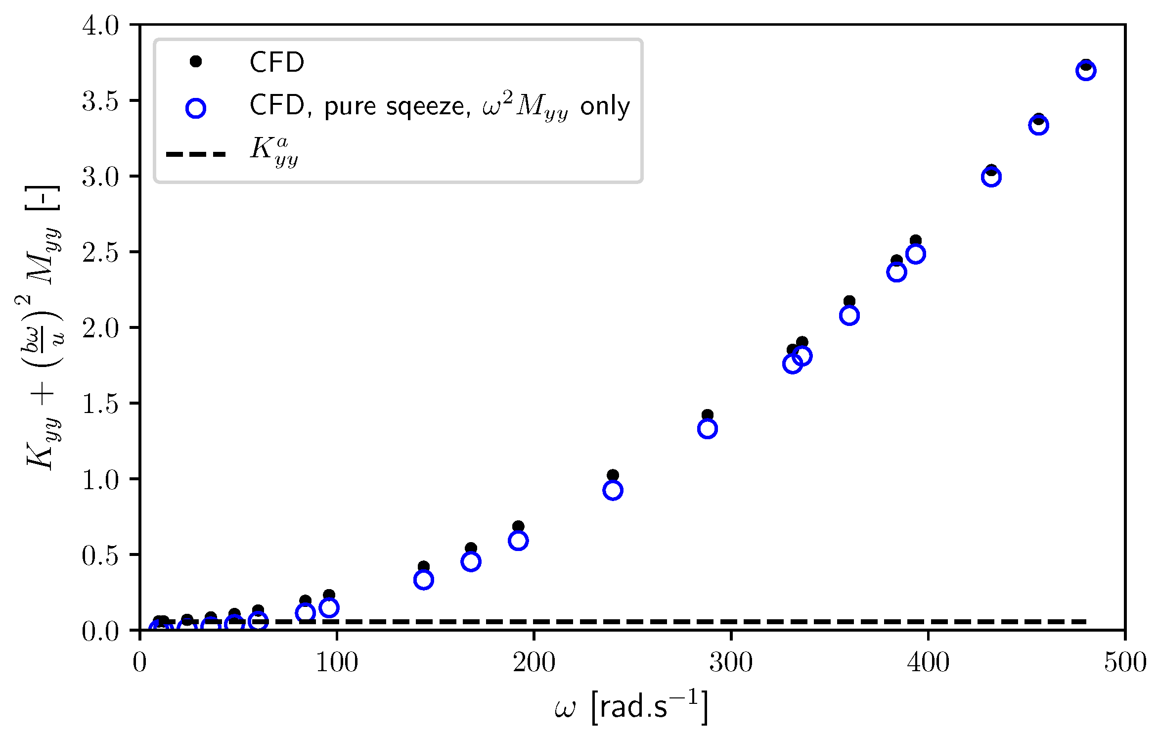
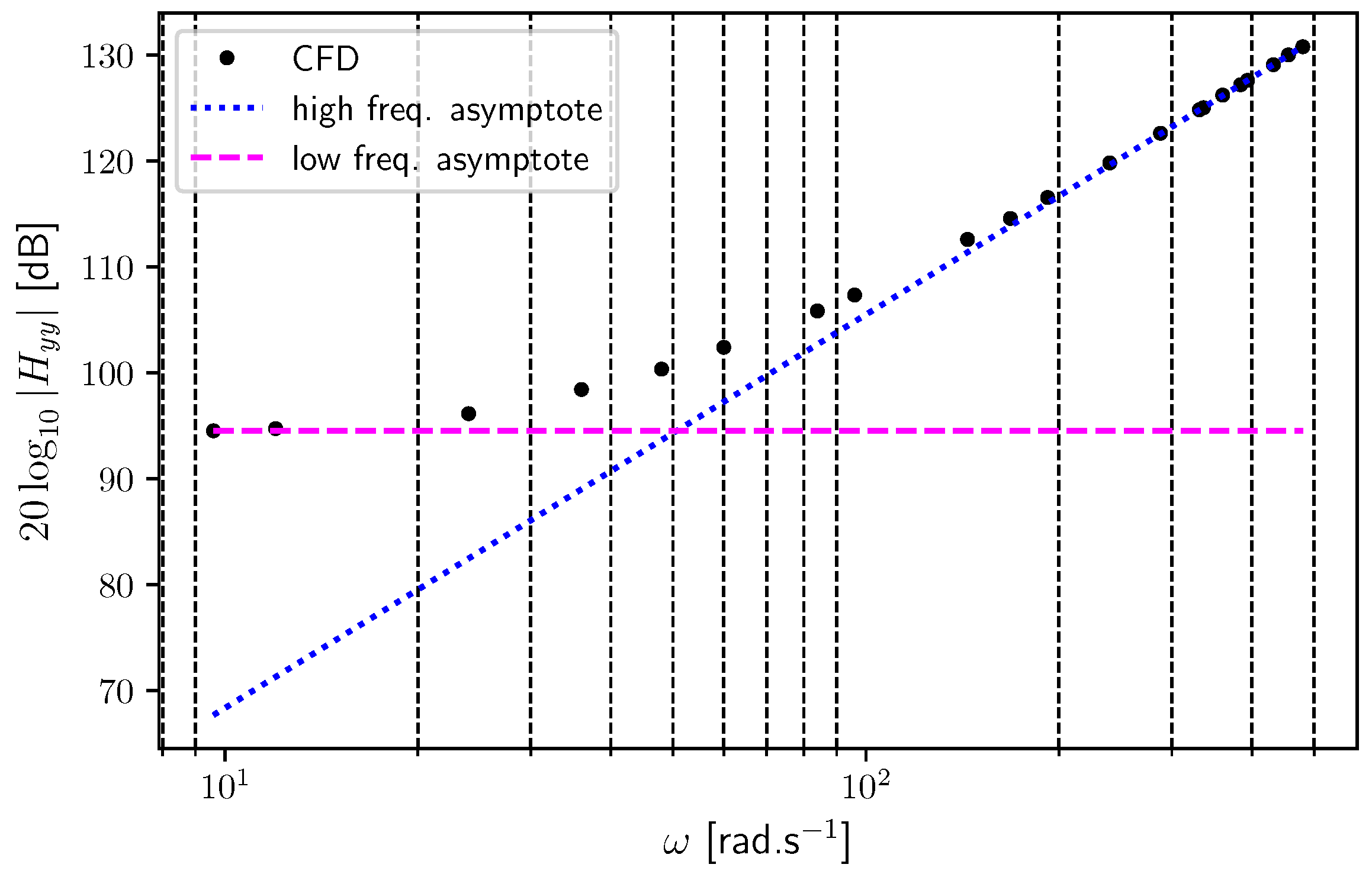
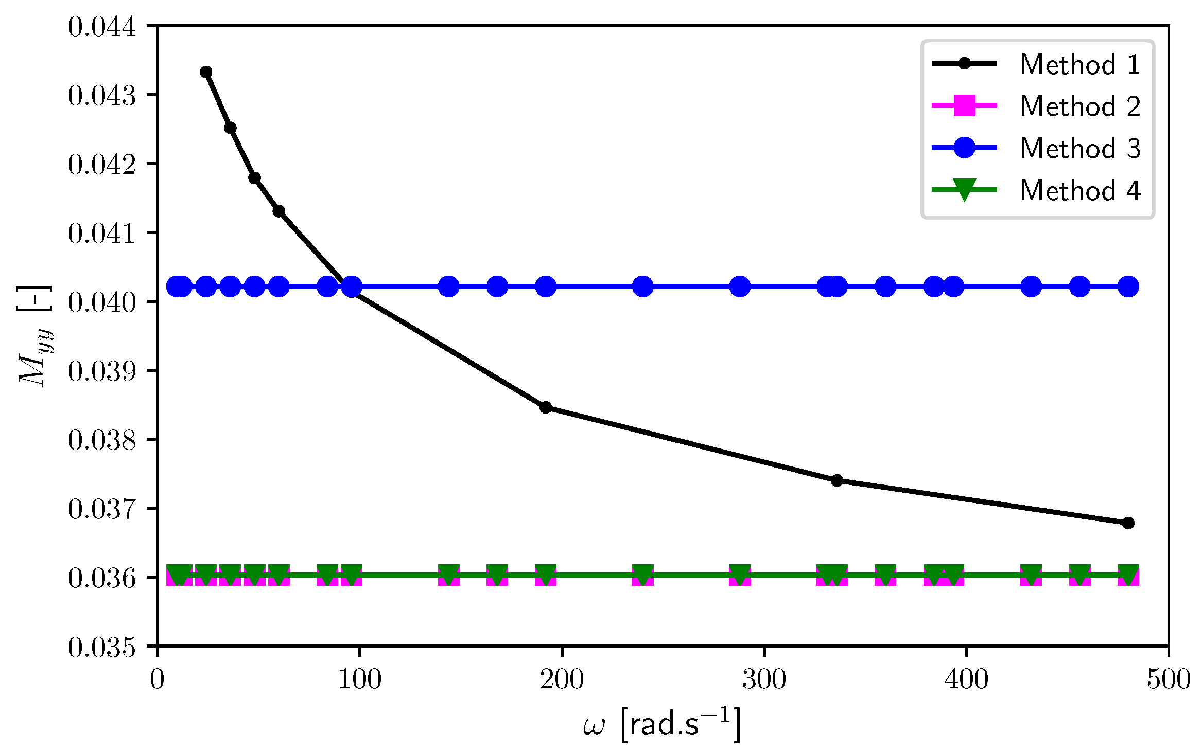
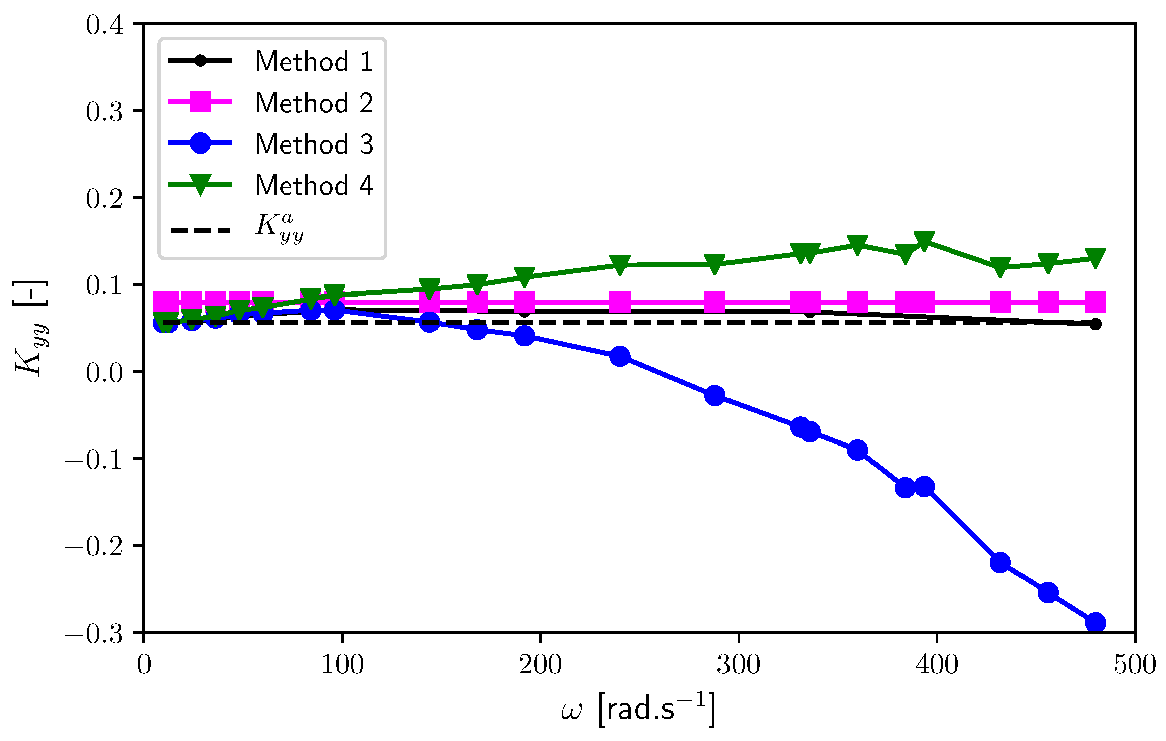
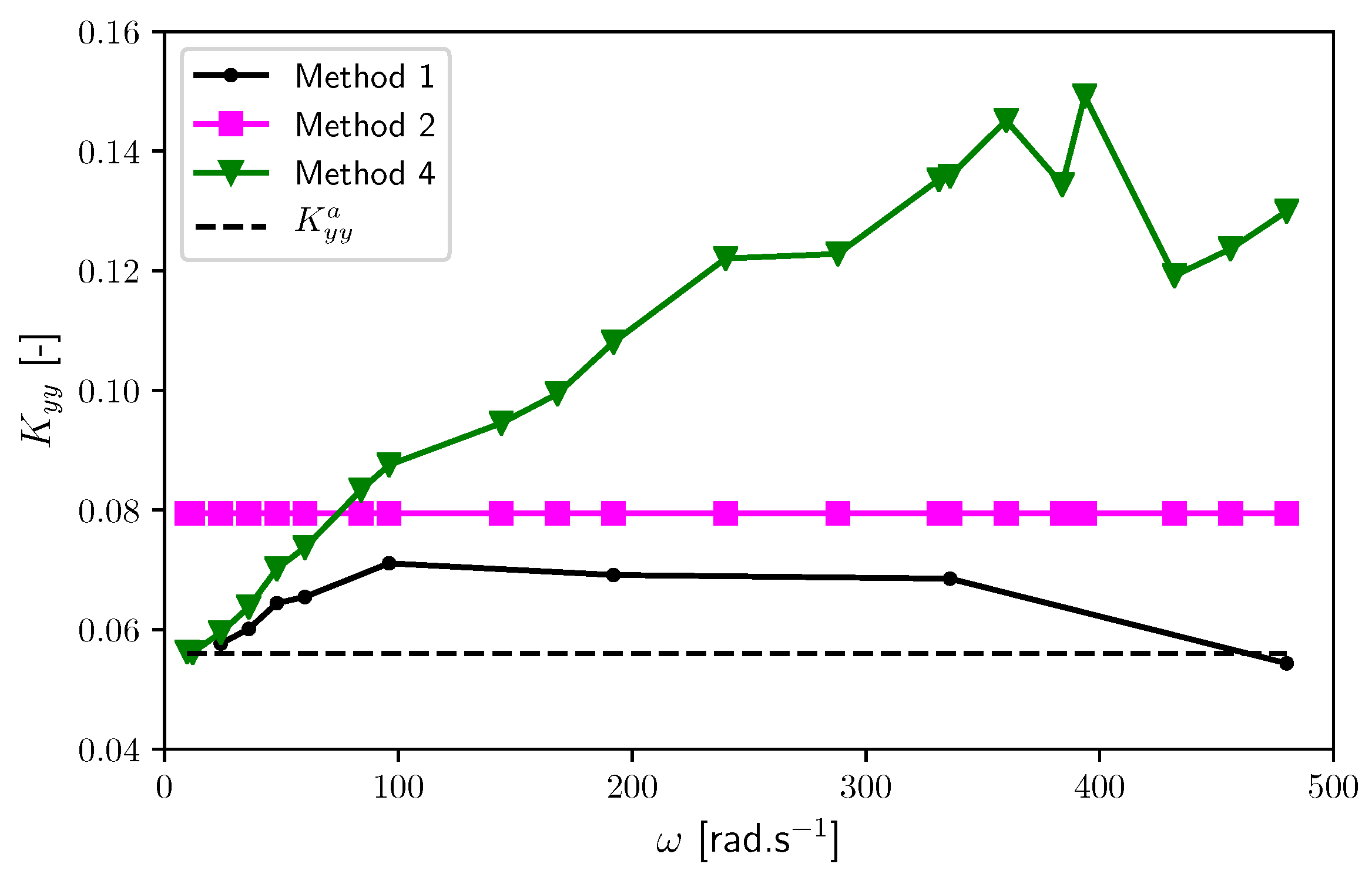
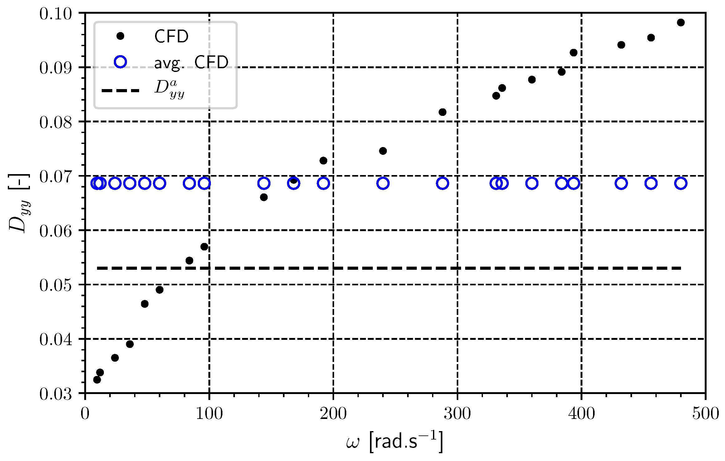
• Alternative methods to separate the dynamic stiffness into added mass and static stiffness effects are investigated. The authors [20] previously demonstrated that temporal inertia effects as embodied in added mass coefficients are inherent within transient CFD simulations. It then becomes necessary to perturb the bearing at multiple frequencies in order to fit the static stiffness and added mass parameters. However, different techniques for fitting the dynamic stiffness will provide different estimates of the coefficients depending on assumed behavior of the coefficients. Details regarding the implementation and robustness of these techniques are explored herein.
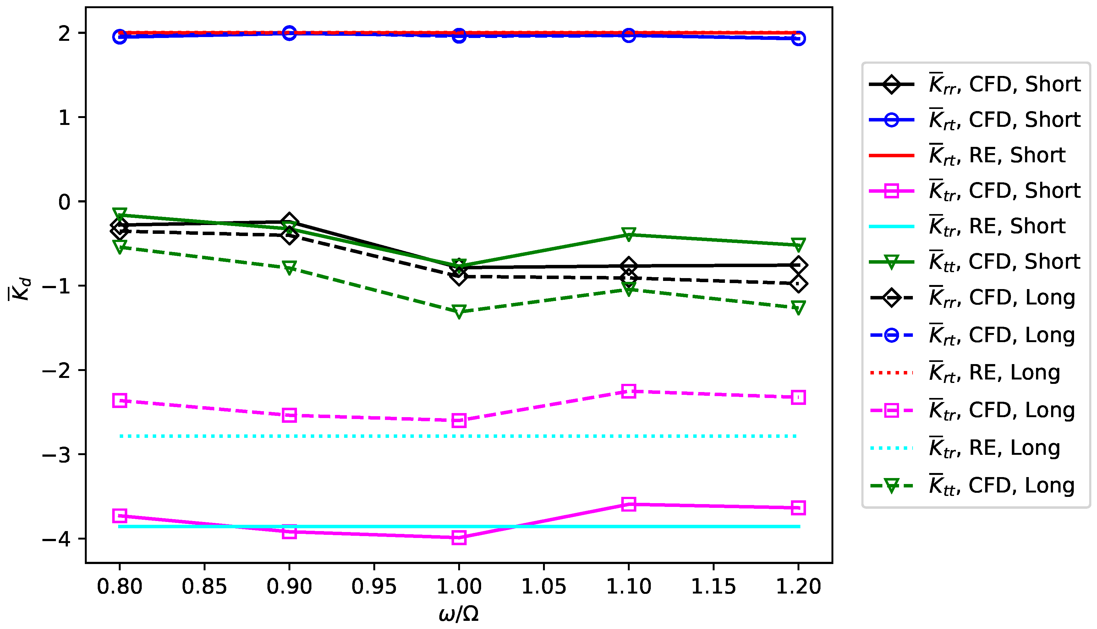
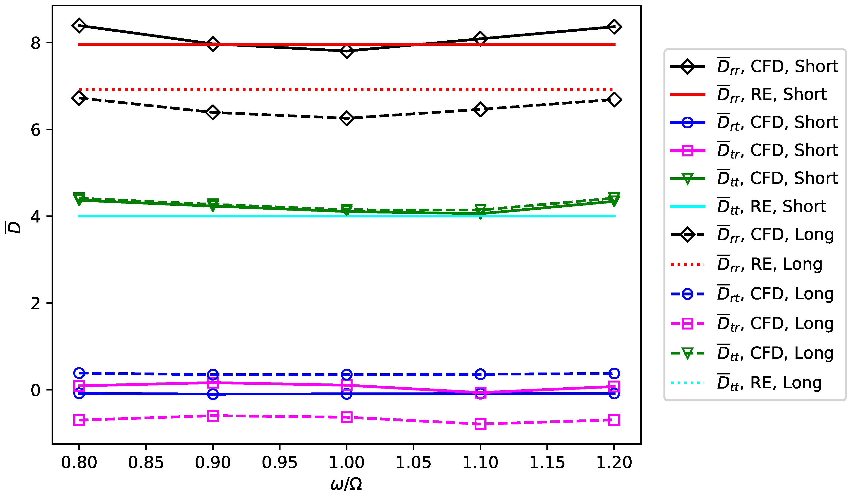
• The proposed methodology is extended to hydrodynamic journal bearing geometries. These bearings are generally of more practical interest than simple slider bearings and an extension of the CFD-based frequency response method to determine the dynamic coefficients is a non-trivial task, warranting a thorough explanation. The dynamic coefficients predicted for short $L/D=0.25$ and long $L/D=3.0$ journal bearing geometries are compared directly with those obtained from the perturbed Reynolds equation.

3. Geometry

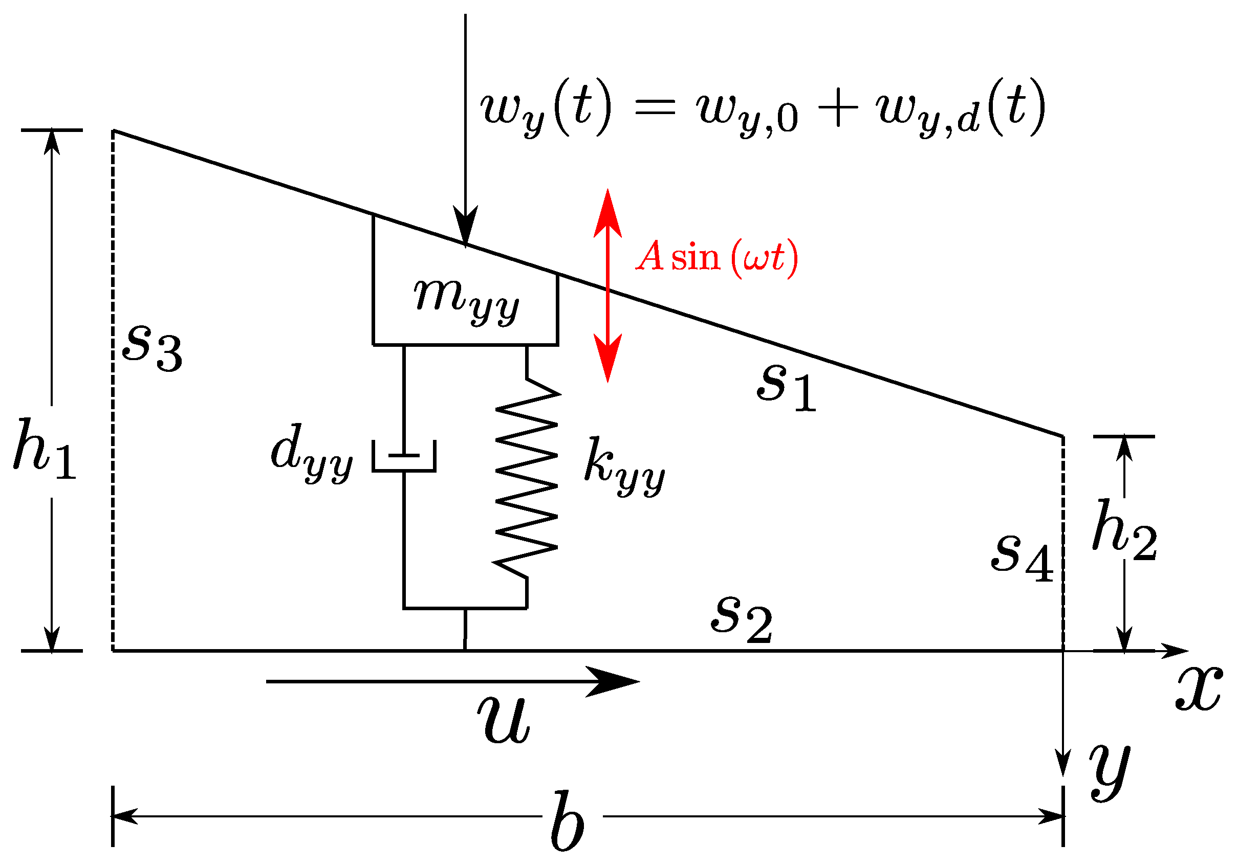
3.1. Linear Slider Bearing

Figure 1 depicts the extremely long linear slider bearing geometry (length L in the z-direction is considered infinite) and a mechanical model of the hydrodynamic fluid film. The geometric and operational parameter values are summarized in

Table 1. Linear slider bearing parameters.

Parameter	Value	Unit
$h_1$	533.4	[$\mathsf{\mu }$m]
$h_2$	266.7	[$\mathsf{\mu }$m]
b	39.22	[mm]
u	1.88	[m·s${}^{-1}$]
A	26.7	[$\mathsf{\mu }$m]
$\nu$	1.004 × 10${}^{-6}$	[m${}^2$·s${}^{-1}$]
$\omega$	varied	[-]

and are motivated by the physical characteristics of rubber-lined, marine bearings where individual staves create a local geometry similar to that of a series of extremely long slider bearings assembled in the circumferential direction.

The lubricant considered is water and the minimum film thickness, $h_2=266.7$ [$\mathsf{\mu }$m], is based on the radial clearance of a marine journal bearing with a diameter of $50.8$ [mm]. For a traditional (oil-lubricated, plain) hydrodynamic journal bearing, the ratio of the radial clearance and the bearing radius, $\frac{C}{R}$, is generally between 1/500 and 1/1000. For marine bearings, $\frac{C}{R}$ is slightly larger (3.4/500) [24]. The nominal bearing width $b=39.22$ [mm] satisfies $\frac{h_2}{b}=\frac{3.4}{500}$ motivated by marine bearing dimensions. Nominally, a bearing taper ratio $r=2.0$ is considered, where $r=h_1/h_2$. The bearing, inflow, and outflow surfaces $s_i$ (where $i=1,2,3,4$) will be subsequently used for identification of CFD boundary conditions.

The sliding velocity $u=1.88$ [m s⁻¹] results from fixing the sliding Reynolds number $R{e}_u=500$ ($Re=\frac{u{h}_2}{\nu }$) which corresponds to a reduced sliding Reynolds number $R{e}_u^{\ast }=3.4$ where $R{e}_u^{\ast }=R{e}_u\left(\frac{h_2}{b}\right)$. Limiting the sliding speed of the bearing renders the flow laminar, eliminating the need, at this stage, for turbulence accounting. For a bearing with a diameter of $50.8$ [mm], a sliding speed $u=1.88$ corresponds to a rotational speed $\mathsf{\Omega }=74$ [rad·s${}^{-1}$] or $706.8$ [rpm]. The rotational speed, while not characteristic in general for bearings, is in the bulk range of speeds developed within marine bearings.

Perturbations are applied to bearing surface $s_1$ with an amplitude A and and frequency $\omega$, which is varied. The oscillation amplitude is taken to be 10% of the minimum film height $h_2$.

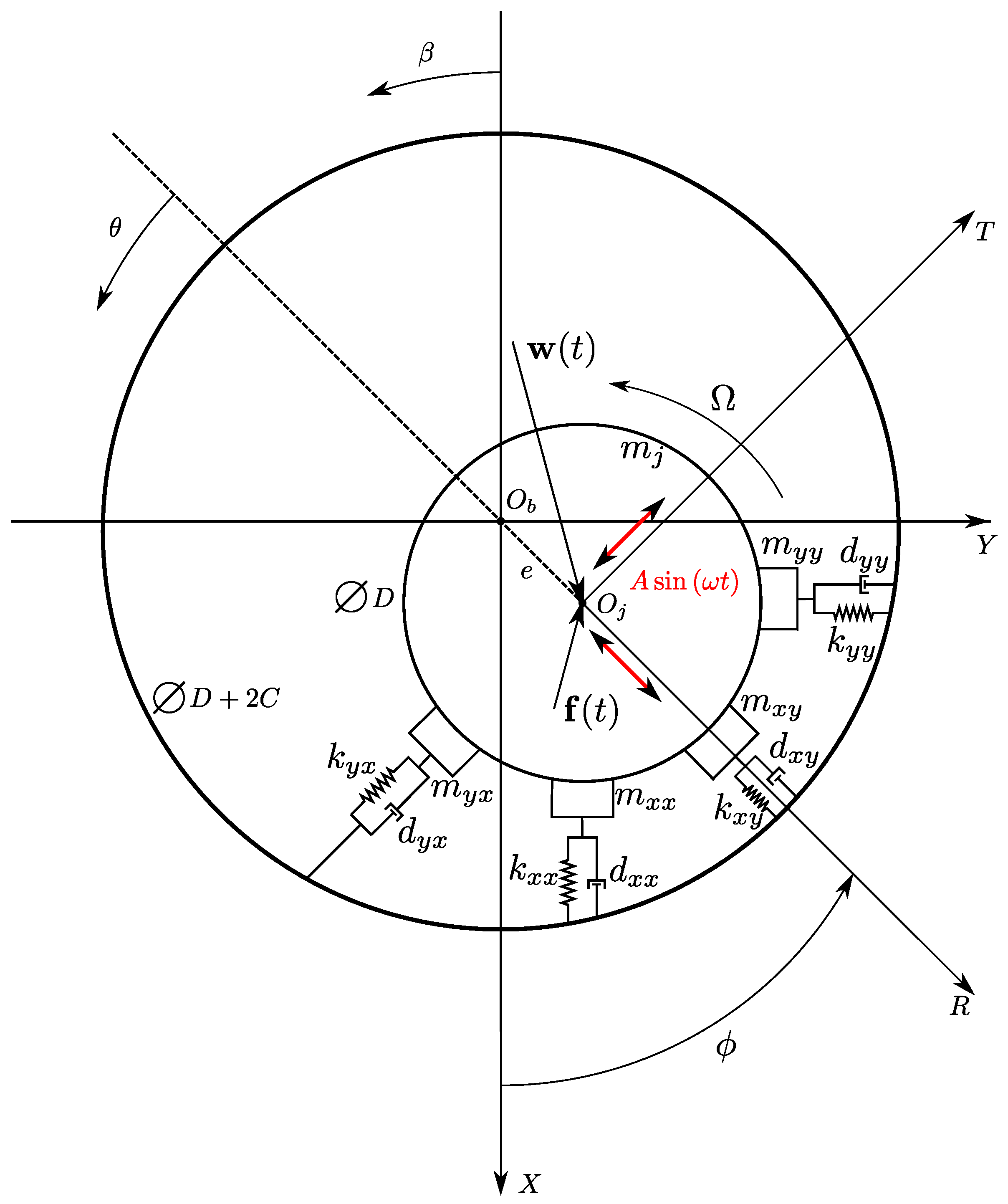
3.2. Journal Bearing

The geometry and mechanical model of the hydrodynamic fluid film of a plain journal bearing is depicted in Figure 2. The journal diameter is D and the radial clearance of the bearing is C. The bearing length is L in the z-direction (not shown). The rotational speed of the bearing is $\mathsf{\Omega }$. The film thickness of the bearing h is defined through the angular coordinate $\theta$ which in-turn is defined by a line extending along the bearing center $O_b$ and the journal center $O_j$ (line-of-centers). The reference frame $(X,Y)$ is fixed (inertial) with its origin located at the bearing center. The reference frame $(R,T)$ is also fixed (inertial) with its origin located at $O_j$ ($O_j$ is translated a distance e from $O_b$) and rotated through an angle $\varphi$ from $(X,Y)$. The position and orientation of reference frame $(R,T)$ is defined in terms of the bearing’s static equilibrium position, which may be expressed as $(x_0,y_0)$ or $(ecos\varphi ,esin\varphi )$ in reference frame $(X,Y)$.

The geometric and parameter values of the journal bearing considered in the present work are summarized in

Table 2. Journal bearing parameters.

Parameter	Value	Unit
C	173	[$\mathsf{\mu }$m]
D	50.8	[mm]
$L/D$	0.25 or 3.0	[-]
$\mathsf{\Omega }$	706.8	[rpm]
$\epsilon =e/C$	0.5	[-]
A	8.636	[$\mathsf{\mu }$m]
$\nu$	1.004 × 10${}^{-6}$	[m${}^2$·s${}^{-1}$]
$\omega$	varied	[-]

.

The bearing clearance C was determined from the nominal value of $C/R$ equal to 0.0068 for a marine bearing and a bearing radius of 25.4 [mm] (i.e., 1 inch). The bearing Reynolds number $Re=\mathsf{\Omega }RC/\nu$ is equal to 323.9. As the linear slider bearing, the flow may be considered laminar, considering $Re=2000$ as the onset for turbulence [25]. Both short and long bearing geometries were investigated, the latter having a $L/D=3.0$, which is typical of marine bearings.

4. Mathematical Modeling

4.1. Dynamic Models

4.1.1. Linear Slider Bearing

A linear mechanical model of the hydrodynamic fluid film dynamic response can be seen in Figure 1. The hydrodynamic film is modeled through a linear spring, damper, and added mass. Applying Newton’s second law to the upper surface $s_1$ considering a small displacement y from the static equilibrium position results in Equation (1) for the dynamic bearing load $w_{y,d}\left(t\right)$.

$$-w_{y,d}\left(t\right)=k_{yy}y\left(t\right)+d_{yy}\dot{y}\left(t\right)+m_{yy}\ddot{y}\left(t\right)$$

(1)

In Equation (1), the mass of the slider has been neglected and slider is constrained to move only in the y-direction and for which the initial position of the upper surface of the bearing $s_1$ is considered zero, $y=0$. A notable feature of Equation (1) is retention of an added mass coefficient associated with inertia of the fluid. Snyder et al. [20] previously demonstrated that lubricant inertia can cause an appreciable difference between the dynamic bearing stiffness ($k_{yy}+m_{yy}{\omega }^2$) predicted using CFD (lubricant inertia present) and the static stiffness ($k_{yy}$) predicted by the perturbed Reynolds equation (lubricant inertia neglected).

In the present work, the dynamic coefficients present in Equation (1) are determined by correlating an applied harmonic displacement (input) with the CFD-predicted force (output). Correlation of the input and output is performed both in the time-domain through curve fitting and in the frequency domain through development of a frequency response function (FRF).

For the time-domain approach, consider the application of a known input displacement (sinusoidal) $y=-Asin\left(\omega t\right)$ to the bearing surface $s_1$ depicted in Figure 1. The sinusoidal displacement may alternatively be expressed as a complex exponential function as $y\left(t\right)=Aexp\{-i\omega t\}$. If the input displacement is a harmonic sinusoidal function, the steady-state output force of this linear model will also be a sinusoidal function which can be written as a complex exponential function $w_{y,d}\left(t\right)=Fexp\{-i(\omega t+\alpha \left)\right\}$, where F is the unknown force amplitude and $\alpha$ is the phase shift of the harmonic force. Substituting the complex exponential forms of the displacement and force into Equation (1) leads to Equations (2) and (3).

$$\left(k_{yy}+{\omega }^2{m}_{yy}\right)=\mathrm{Re}\left[\frac{F}{A}exp\{-i\alpha \}\right]$$

(2)

$$d_{yy}=-\frac{\mathrm{Im}\left[\frac{F}{A}exp\{-i\alpha \}\right]}{\omega }$$

(3)

Alternatively, the dynamic stiffness and damping coefficients can be determined using a frequency domain approach through the establishment of a frequency response function (FRF), $H_{yy}(-i\omega )$ as in Equation (4).

$$\frac{W_{y,d}(-i\omega )}{Y(-i\omega )}=H_{yy}(-i\omega )=k_{yy}-i\omega d_{yy}+{\omega }^2{m}_{yy}$$

(4)

The dynamic stiffness and damping coefficients are then determined from the real and imaginary components of $H_{yy}$ as given by Equations (5) and (6).

$$\left(k_{yy}+{\omega }^2{m}_{yy}\right)=\mathrm{Re}\left[H_{yy}(-i\omega )\right]$$

(5)

$$d_{yy}=-\frac{\mathrm{Im}\left[H_{yy}(-i\omega )\right]}{\omega }$$

(6)

In order to separate the dynamic stiffness into static stiffness and added mass components, the perturbation frequency $\omega$ is varied. Several techniques are investigated to separate the dynamic stiffness within the Results section.

The stiffness, damping, and added mass coefficients per unit length (e.g., $k_{yy}$ has units [N/m/m] are expressed in non-dimensional form through Equations (7)–(9), respectively [26].

$$K_{yy}=\frac{h_2^3{k}_{yy}}{6\mu u{b}^2}$$

(7)

$$D_{yy}=\frac{h_2^3{d}_{yy}}{6\mu u{b}^2}\left(\frac{u}{b}\right)=\frac{h_2^3{d}_{yy}}{6\mu b^3}$$

(8)

$$M_{yy}=\frac{h_2^3{m}_{yy}}{6\mu u{b}^2}{\left(\frac{u}{b}\right)}^2=\frac{h_2^{3}u{m}_{yy}}{6\mu b^4}$$

(9)

In Equations (7)–(9), $\mu =0.001$ [Pa·s] is the dynamic viscosity of the water lubricant.

4.1.2. Journal Bearing

The journal depicted in Figure 2 is subject to a dynamic load $\mathbf{w}\left(t\right)$ and the net force generated by the hydrodynamic film is $\mathbf{f}\left(t\right)$. If the film force $\mathbf{f}\left(t\right)$ is linearized through a Taylor Series expansion and expressed in terms of linearized dynamic coefficients (stiffness, damping, and added mass), the Equations of motion may be expressed in matrix form as Equation (10).

$$\left[\begin{array}{cc}{m}_{xx}& m_{xy}\\ m_{yx}& m_{yy}\end{array}\right]\left\{\begin{array}{c}\ddot{x}\\ \ddot{y}\end{array}\right\}+\left[\begin{array}{cc}{d}_{xx}& d_{xy}\\ d_{yx}& d_{yy}\end{array}\right]\left\{\begin{array}{c}\dot{x}\\ \dot{y}\end{array}\right\}+\left[\begin{array}{cc}{k}_{xx}& k_{xy}\\ k_{yx}& k_{yy}\end{array}\right]\left\{\begin{array}{c}x\\ y\end{array}\right\}=\left[\begin{array}{cc}{m}_j& 0\\ 0& m_j\end{array}\right]\left\{\begin{array}{c}\ddot{x}\\ \ddot{y}\end{array}\right\}-\left\{\begin{array}{c}{w}_{d,x}\left(t\right)\\ w_{d,y}\left(t\right)\end{array}\right\}$$

(10)

More succinctly, Equation (10) can be expressed as Equation (11).

$$\mathbf{M}\ddot{\mathbf{x}}+\mathbf{D}\dot{\mathbf{x}}+\mathbf{K}\mathbf{x}={\mathbf{M}}_{\mathbf{j}}\ddot{\mathbf{x}}-{\mathbf{w}}_d\left(t\right)$$

(11)

In Equation (11), $\mathbf{M}$ and ${\mathbf{M}}_j$ represent the added mass (fluid inertia) matrix and the journal mass matrix, respectively. Unlike in an experiment, a massless journal (${\mathbf{M}}_j=0$) can be simulated using CFD and in conjunction with Equation (11) can be reduced to Equation (12).

$$\mathbf{M}\ddot{\mathbf{x}}+\mathbf{D}\dot{\mathbf{x}}+\mathbf{K}\mathbf{x}=-{\mathbf{w}}_d\left(t\right)$$

(12)

If a sinusoidal displacement of complex form $\mathbf{q}=\mathbf{X}\left(i\omega \right)exp\left(i\omega t\right)$ is applied to the journal, then the corresponding output force will also be sinusoidal, ${\mathbf{w}}_d\left(t\right)=\mathbf{W}\left(i\omega \right)exp\left(i\omega t\right)$. $\mathbf{X}\left(i\omega \right)$ and $\mathbf{W}\left(i\omega \right)$ are the complex amplitude vectors of the input displacement and the output force, respectively. Substituting these expressions into Equation (12), results into Equation (13).

$$\left({\omega }^2\mathbf{M}-i\omega \mathbf{D}+\mathbf{K}\right)\mathbf{X}\left(i\omega \right)=-\mathbf{W}\left(i\omega \right)$$

(13)

Substituting the frequency response function matrix $\mathbf{H}\left(i\omega \right)=(\mathbf{K}+{\omega }^2\mathbf{M})-i\omega \mathbf{D}$ into Equation (13) results in Equation (14).

$$\mathbf{H}\left(i\omega \right)=-\frac{\mathbf{W}\left(i\omega \right)}{\mathbf{X}\left(i\omega \right)}$$

(14)

The dynamic stiffness and damping coefficients can be evaluated at different perturbation frequencies ${\omega }_i$ using Equations (15) and (16), respectively.

$$\mathbf{K}+{\omega }^2\mathbf{M}=\mathrm{Re}\left(\mathbf{H}\left(i{\omega }_i\right)\right)$$

(15)

$$\mathbf{D}=-\frac{\mathrm{Im}\left(\mathbf{H}\left(i{\omega }_i\right)\right)}{{\omega }_i}$$

(16)

The preceding development involved the determination of the the dynamic coefficients in the fixed $(X,Y)$ reference frame of Figure 2. However, results from the CFD model are easiest to obtain through the application of a static eccentricity along a single coordinate direction. Setting up the CFD model in this manner means that the dynamic coefficients which result will be in the $(R,T)$ reference frame of Figure 2. A coordinate transformation is necessary to move from $(O_j,R,T)$ to $(O_b,X,Y)$. Equations (17) and (18) summarize the transformation of the stiffness matrix from the $(X,Y)$ to $(R,T)$ and from the $(R,T)$ to $(X,Y)$ reference frames, respectively. Identical transformations also apply to the added mass and damping matrices.

$$\tilde{\mathbf{K}}={\mathbf{T}}_{\varphi }\mathbf{K}{\mathbf{T}}_{\varphi }^T$$

(17)

$$\mathbf{K}={\mathbf{T}}_{\varphi }^T\tilde{\mathbf{K}}{\mathbf{T}}_{\varphi }$$

(18)

where the rotation matrix is given by

$${\mathbf{T}}_{\varphi }=\left[\begin{array}{cc}cos\varphi & sin\varphi \\ -sin\varphi & cos\varphi \end{array}\right]$$

(19)

The stiffness, damping, and added mass matrices will be presented in dimensionless for as given in Equations (20)–(22), respectively [4].

$$\overline{\mathbf{K}}=\frac{\mathbf{K}C}{W_0}$$

(20)

$$\overline{\mathbf{D}}=\frac{\mathbf{D}C\mathsf{\Omega }}{W_0}$$

(21)

$$\overline{\mathbf{M}}=\frac{\mathbf{M}C{\mathsf{\Omega }}^2}{W_0}$$

(22)

In Equations (20)–(22), $\mathsf{\Omega }$ is the shaft rotational speed in radians per second, and $W_0$ is the static load carrying capacity of the bearing.

4.2. Hydrodynamic Fluid Film

The hydrodynamic fluid film is resolved by solving an advectiveless form ($(\mathbf{v}·\nabla )\mathbf{v}=0$) of the Navier–Stokes equations given in Equations (23) and (24) under the assumptions of a Newtonian, incompressible, isothermal fluid.

$$\nabla ·\mathbf{v}=0$$

(23)

$$\frac{\partial \mathbf{v}}{\partial t}=\mathbf{f}-\nabla \left(\frac{p}{\rho }\right)+\nu {\nabla }^2\mathbf{v}$$

(24)

In the absence of the temporal inertia term, $\frac{\partial \mathbf{v}}{\partial t}$, the resulting set of equations are known as Stokes equations and were used to analyze the flow around spherically shaped pendulums [27] in creeping flow ($Re\to 0$). The Stokes equations are at the basis of the genesis of the Reynolds equation, which is commonly employed in hydrodynamic lubrication. The difference resides in the fact that while the Reynolds equation is integrated across the film, and thus rendered two-dimensional, Stokes equations preserve their 3D character.

In hydrodynamic bearings resolved using CFD with ever-present temporal inertia, it is necessary to take the inertia effects into consideration through the addition of added mass terms within the mechanical model of the fluid film. The added mass elements may or may not significantly influence the dynamic stiffness depending on the bearing geometry and operating conditions. If significant, the added mass terms must be separated from the dynamic stiffness to determine the static stiffness elements.

5. Numerical Model Setup

5.1. CFD Solver

Steady and transient forms of the Navier–Stokes and Stokes equations are solved using the open-source continuum mechanics library OpenFOAM [28] version 5.0. The three dimensional form of the equations are discretized on a boundary conforming, non-overlapping computational mesh using the finite volume method. The meshing application blockMesh is used to generate the mesh using hexahedral cells. “Infinitely long” models are achieved by spanning the z direction of the computational domain with a single cell in conjunction with the specification of “empty” boundary conditions (OpenFOAM terminology) on the associated axial boundaries.

The OpenFOAM application applied in the analysis is termed “pimpleDyMFoam” which solves the incompressible form of the Navier–Stokes equations (modified with removal of advective inertia) on a dynamic (moving) mesh. The solver is a pressure-based, predictor-corrector algorithm based on a combination of PISO [29] and SIMPLE [30,31] algorithms. For details regarding the specific discretization schemes and solver parameters, the interested reader is referred to [20].

5.2. Boundary Conditions

The application of the various boundary condition types to specific surfaces (patches) within the CFD models are summarized in

Table 3. Linear slider bearing OpenFOAM boundary conditions. See Figure 1 for model surfaces identification names. Boundary conditions values are required for the velocity U, the pressure P, and displacement D fields directly (Dirchlet) or their gradients (Neumann). For the extremely long model, the “Front” and “Back” (not included in table) are specified as “empty”.

Boundary	U	P	D
$s_1$	movingWallVelocity; value uniform (0 0 0);	zeroGradient;	oscillatingDisplacement; amplitude (0 2.667 $\times {10}^{-5}$ 0) omega varied; value uniform (0 0 0);
$s_2$	fixedValue; value uniform (1.88 0 0);	zeroGradient;	fixedValue; value uniform (0 0 0);
$s_3$	pressureInletOutletVelocity; value uniform (0 0 0);	fixedValue; value uniform 0;	slip;
$s_4$	pressureInletOutletVelocity; value uniform (0 0 0);	fixedValue; value uniform 0;	slip.

and

Table 4. Journal bearing OpenFOAM boundary conditions. Boundary conditions are required for the velocity U, the pressure P, and displacement D. “Front” and “Back” refer to the axial ends of the bearing.

Boundary	U	P	D
Journal	movingWallVelocity; value uniform (0 0 0);	zeroGradient;	oscillatingDisplacement; amplitude (0 2.667 $\times {10}^{-5}$ 0) omega varied; value uniform (0 0 0);
Bearing	rotatingWallVelocity; origin; axis (0 0 1); omega 74.016; value uniform (0 0 0);	zeroGradient;	fixedValue; value uniform (0 0 0);
Front	pressureInletOutletVelocity; value uniform (0 0 0);	fixedValue; value uniform 0;	slip;
Back	pressureInletOutletVelocity; value uniform (0 0 0);	fixedValue; value uniform 0;	slip.

for the linear slider bearing and the journal bearing, respectively.

5.2.1. Linear Slider Bearing

5.2.2. Journal Bearing

The journal bearing CFD model is setup with a prescribed (fixed) eccentricity in the r direction in the coordinate system as introduced in Figure 2. Note that $(R,T)$ coordinate system as introduced in Figure 2 corresponds to an $(X,Y)$ reference system of the CFD simulation. Also, note that within the CFD model, journal rotation is not applied directly, but rather, rotational velocity is applied in the opposite direction to the bearing. Alternatively, if the journal were supplied with rotational velocity and oscillating displacement, a new boundary condition would have to be implemented within OpenFOAM.

5.3. Numerical Accuracy Quantification

5.3.1. Linear Slider Bearing

Verification of the CFD model of the linear slider bearing requires consideration of three primary factors: spatial convergence, local temporal convergence, and global temporal convergence. Spatial convergence refers to a mesh density which adequately resolves the discrete approximations of the spatial derivatives in the model (differential) equations. Local temporal convergence refers to a time step which adequately resolves the discrete approximations of the temporal derivatives in the model (differential) equations. Spatial and local temporal convergence are typical metrics associated with the accuracy of CFD results. The additional consideration of global temporal convergence is required as the dynamic CFD results will be fit to a model. The global temporal convergence is related to the number of oscillating periods of the boundary perturbation.

For all three factors, the dynamic stiffness and the damping coefficients are metrics of interest. Spatial and temporal convergence is quantified for a single perturbation frequency of 48 [rad·s${}^{-1}$].

Table 5. Dynamic coefficient variation with mesh density. Five periods and 200 time steps per period.

${\mathit{N}}_{\mathbf{cells}}$	Curve-Fit		FRF
	${\mathit{K}}_{\mathit{yy}}\mathbf{+}{\mathit{\omega }}^{\mathbf{2}}{\mathbf{M}}_{\mathit{yy}}$	${\mathit{D}}_{\mathit{yy}}$	${\mathit{K}}_{\mathit{yy}}\mathbf{+}{\mathit{\omega }}^{\mathbf{2}}{\mathit{M}}_{\mathit{yy}}$	${\mathit{D}}_{\mathit{yy}}$
1470 (147 × 10)	$1.054\times {10}^{-1}$	$4.263\times {10}^{-2}$	$1.031\times {10}^{-1}$	$4.500\times {10}^{-2}$
3315 (221 × 15)	$1.062\times {10}^{-1}$	$4.399\times {10}^{-2}$	$1.039\times {10}^{-1}$	$4.644\times {10}^{-2}$
5880 (294 × 20)	$1.066\times {10}^{-1}$	$4.451\times {10}^{-2}$	$1.042\times {10}^{-1}$	$4.700\times {10}^{-2}$

,

Table 6. Dynamic coefficient variation with number of time steps per period. Five periods with a 221 × 15 mesh.

${\mathit{N}}_{\mathbf{tsteps}\mathbf{/}\mathbf{period}}$	Curve-Fit		FRF
	${\mathit{K}}_{\mathit{yy}}\mathbf{+}{\mathit{\omega }}^{\mathbf{2}}{\mathit{M}}_{\mathit{yy}}$	${\mathit{D}}_{\mathit{yy}}$	${\mathit{K}}_{\mathit{yy}}\mathbf{+}{\mathit{\omega }}^{\mathbf{2}}{\mathit{M}}_{\mathit{yy}}$	${\mathit{D}}_{\mathit{yy}}$
100	$1.052\times {10}^{-1}$	$4.538\times {10}^{-2}$	$1.028\times {10}^{-1}$	$4.785\times {10}^{-2}$
200	$1.062\times {10}^{-1}$	$4.399\times {10}^{-2}$	$1.039\times {10}^{-1}$	$4.644\times {10}^{-2}$
300	$1.066\times {10}^{-1}$	$4.353\times {10}^{-2}$	$1.062\times {10}^{-1}$	$4.440\times {10}^{-2}$

and

Table 7. Dynamic coefficient variation with number of periods. Two hundred time steps per period with a 221 × 15 mesh.

${\mathit{N}}_{\mathbf{period}}$	Curve-Fit		FRF
	${\mathit{K}}_{\mathit{yy}}\mathbf{+}{\mathit{\omega }}^{\mathbf{2}}{\mathit{M}}_{\mathit{yy}}$	${\mathit{D}}_{\mathit{yy}}$	${\mathit{K}}_{\mathit{yy}}\mathbf{+}{\mathit{\omega }}^{\mathbf{2}}{\mathit{M}}_{\mathit{yy}}$	${\mathit{D}}_{\mathit{yy}}$
3	$1.056\times {10}^{-1}$	$4.475\times {10}^{-2}$	$1.022\times {10}^{-1}$	$4.837\times {10}^{-2}$
5	$1.062\times {10}^{-1}$	$4.399\times {10}^{-2}$	$1.039\times {10}^{-1}$	$4.644\times {10}^{-2}$
8	$1.065\times {10}^{-1}$	$4.345\times {10}^{-2}$	$1.049\times {10}^{-1}$	$4.511\times {10}^{-2}$

, respectively summarized the impact of mesh density, time step size, and number of simulated periods on the predicted dimensionless dynamic coefficients. Dynamic coefficients predicted using both the time-domain curve-fit method and the frequency response function are presented.

In general, the damping coefficients are more sensitive to the numerical parameters than the dynamic stiffness. Additionally, the FRF method is marginally more sensitive to the numerical parameters than the curve-fit method. Overall, using the mesh density of 221 × 15 with five periods of oscillation and 200 time steps per oscillation will result in numerical errors below 2% (for the curve-fit method). This setup for the mesh density and temporal parameters was chosen as it can be used to predict dynamic coefficients will less than 5% numerical error with reasonably low computational overhead (each case takes approximately 30 minutes using four threads on a Intel i7-4790 3.6 GHz CPU).

In all cases, the perturbation amplitude was set to 10% of the minimum film thickness $h_2$. The predicted dynamic coefficients remained unchanged reducing the oscillation amplitude from 10% to 5% of the minimum film thickness. Thus, for a perturbation amplitude of 10% of the minimum film thickness, the dynamic response of the hydrodynamic film is linear with respect to perturbation amplitude.

The nominal model setup with a mesh density of 221 × 15, five oscillation periods, and 200 time steps per oscillation, the curve-fit and FRF methods predict dynamic stiffness and damping coefficients which differ by 2.2% and 5.6%, respectively. Proceeding, the FRF results will be presented owing to the generality of the method and prevalence in experimental parameter identification techniques.

5.3.2. Journal Bearing

The short journal bearing model (Table 2 was ran with time step size of 1 $\times {10}^{-5}$ [s] with five periods of oscillation. Dynamic coefficients evaluated with a mesh density of 20,000 cells (10 × 100 × 20, “across-film” × ”circumferential” × ”axial”) all fell within 2% of the those coefficients predicted using a mesh with 90,000 cells (15 × 200 × 30). For the long journal bearing, the mesh density was 10 × 100 × 120 and like the short bearing, the predicted dynamic coefficients fell within 2% of a finer, 15 × 100 × 120 mesh.

6. Results and Discussion

6.1. Linear Slider Bearing (Extremely Long)

The stiffness and damping coefficients predicted using CFD are compared against the analytic results yielded by Equations (25) and (26), respectively.

$$K_{yy}^a=-\frac{h_2^3{(x_2-x_1)}^3}{b^2{x}_1{x}_2{\beta }^3{(x_1+x_2)}^2}$$

(25)

$$D_{yy}^a=\frac{2h_2^3}{b^3{\beta }^3}\left(log\frac{x_2}{x_1}+2\frac{x_1-x_2}{x_1+x_2}\right)$$

(26)

where $\beta =(h_2-h_1)/b$, $x_1=h_1/\beta$, and $x_2=h_2/\beta$. Equations (25) and (26) were obtained analytically from the solution of the perturbed Reynolds equation simplified for an infinitely long slider bearing geometry [32].

The dynamic stiffness of the linear slider bearing is plotted with respect to perturbation frequency in Figure 3. The perturbation frequency was varied from 4.8 to 480 [rad·s${}^{-1}$]. The dynamic stiffness exhibits quadratic dependence on perturbation frequency consistent with the presence of an added mass contribution as evidenced by the form of the dynamics stiffness, $K_{yy}+{\omega }^2{M}_{yy}$. At the low frequency limit, the dynamic stiffness approaches the static value. Also plotted in Figure 3 are the CFD results with the linear slider bearing undergoing pure squeeze motion (no sliding velocity) and the analytic dynamic stiffness, i.e., the static stiffness. Under pure squeeze motion, the added mass effect is isolated and its significant contribution to the dynamic stiffness is highlighted. Moreover, it is apparent from the figure that the pure squeeze results can be utilized to separate the static stiffness and added mass coefficients from the dynamic stiffness.

Several methods can be applied in estimating the added mass coefficients from the dynamic stiffness variation with perturbation frequency and are summarized below.

Method 1: The added mass coefficient is evaluated at each perturbation frequency from the pure squeeze CFD results. Using this technique, the added mass coefficient as well and as the static stiffness may exhibit frequency dependence. In this method, at each perturbation frequency, the dynamic stiffness predicted from the pure-squeeze CFD simulation is assumed to equal ${\omega }^2{M}_{yy}$. Thus, the added mass coefficient is determined at the given excitation frequency. Then, this quantity is subtracted from the dynamic stiffness considering both squeeze and sliding, $K_{yy}+{\omega }^2{M}_{yy}$, leaving the static stiffness, $K_{yy}$.

Method 2: The added mass coefficient and the static stiffness are estimated from direct curve-fitting of a quadratic function to the dynamic stiffness. Using this technique, the predicted static stiffness coefficient is $K_{yy}=0.079$ and added mass coefficient is $M_{yy}=0.036$. In this method, a function of the form $p_1+{\omega }^2{p}_2$ is fit to the dynamic stiffness results using a nonlinear least squares method (SciPy [33] (v1.10) based on the algorithm of Moré [34]. The curve-fit parameters $p_1$ and $p_2$ which result correspond to the static stiffness and the added mass coefficients, respectively.

Method 3: The added mass coefficient is estimated using the average difference between the CFD results and the CFD results subject to pure squeeze motion. This method is similar to Method 1, except that the pure squeeze results for the added mass coefficient are averaged over the perturbation frequency. This results in a single estimate for the added mass coefficient. Then, the added mass contribution estimated from this single added mass coefficient is subtracted from the dynamic stiffness.

Method 4: The asymptotic behavior of the frequency response function, $H_{yy}$, in the high frequency limit is used to estimate the added mass coefficient [35]. In this method, the added mass coefficient is estimated using the Bode magnitude plot of the $H_{yy}$ as depicted in Figure 4. The bode plot is consistent with the second-order linear system [36] model assumed for hydrodynamic fluid film, and the plot exhibits both low and high-frequency asymptotic behavior.

The high frequency asymptote corresponding to Figure 4 is given by Equation (27), which is the equation for a linear line where the y-intercept is $31.18$ and the slope is $37.15$.

$$20{log}_{10}|H_{yy}|=31.18+37.15{log}_{10}\left(\omega \right)$$

(27)

At the high frequency limit, the added mass coefficient dominates $H_{yy}$ as the added mass contribution is proportional to ${\omega }^2$, whereas the the damping and stiffness terms are multiplied by $\omega$ and one, respectively. The dominance of the added mass term are higher frequencies assumes that the dynamic coefficients themselves are frequency independent [16,37], or only mildly dependent on perturbation frequency. In the high frequency limit, the $H_{yy}$ may be approximated by Equation (28).

$${\left.H_{yy}\right|}_{\omega \to \infty }\approx {\omega }^2{m}_{yy}$$

(28)

Combining Equations (27) and (28) at the largest value of $\omega$ (480 [rad·s${}^{-1}$]) results in a dimensionless added mass coefficient $M_{yy}=0.04$.

The added mass coefficients estimated using each of the four methods are summarized in Figure 5. Estimating the added mass coefficient using either a direct curve-fit of the dynamic stiffness (Method 2) or using a high-frequency asymptote (Method 4) provides nearly the same result. Making use of the pure squeeze CFD results (Methods 1 and 3) result in higher estimates of the added mass coefficient. As clearly indicated in Figure 5, only Method 1 retains the frequency dependence of the added mass coefficient.

If the added mass coefficient estimates in Figure 5 are used to remove the added mass components from Figure 3, the result is the static stiffness depicted in Figure 6. The negative static stiffness values predicted by Method 3 are non-physical for the linear slider bearing geometry. This indicates that the added mass coefficient is overestimated by averaging the pure squeeze CFD results over the range of perturbation frequencies considered.

Figure 7 is a plot of static stiffness with respect to perturbation frequency with Method 3 removed. In this plot, Method 1 and Method 2 result in static stiffness estimates that fall within 20–30% of the analytic solution (perturbed Reynolds equation). If the added mass coefficient is considered constant and subtracted from the frequency dependent dynamic stiffness (as in Method 4), the static stiffness estimated from CFD is approximately 2× the value stemming from the perturbed Reynolds equation. It seems either Method 1 or Method 2 is most appropriate in estimating the dynamic coefficients. Methods 1 assumes that both $K_{yy}$ and $M_{yy}$ vary with perturbation frequency. Method 1, however, is computationally expensive as it requires both sliding and pure squeeze results be obtained at each perturbation frequency. Method 2 assumes that both $K_{yy}$ and $M_{yy}$ are both frequency independent and fits both parameters over the entire range of perturbation frequencies and seems to provide reasonable estimates for both static stiffness and added mass coefficients. By contrast, Methods 3 and 4 assume that $M_{yy}$ is constant (only), and $K_{yy}$ is either drastically under- or over-estimated at high perturbation frequencies. In the low frequency limit, Methods 1, 3, and 4 appear to converge to the analytic solution.

Figure 8 shows the dimensionless damping coefficient variation with perturbation frequency. The damping coefficient exhibits greater frequency dependence from 0 to 200 [rad·s${}^{-1}$] compared to the frequency range from 200 to 480 [rad·s${}^{-1}$], with the damping coefficient appearing to approach a constant asymptotic value in the higher frequency regime. The CFD-predicted damping coefficient is lower than the perturbed Reynolds equation result in the low frequency range and higher in the high frequency range with a cross-over perturbation frequency occurring somewhere between 60 and 80 [rad·s${}^{-1}$]. As also evidenced in Figure 10 for the short journal bearing, the damping coefficients predicted using CFD and the perturbed Reynolds equation compare closest when the pertubation frequency coincides with the rotational frequency of the shaft. There appears to be some significance to the frequency at which the CFD- and Reynolds equation-predicted damping coefficients coincide and will be investigated in a future work. The coincidence appears to be related to the transition between sub- and super-synchronous excitation and/or the dominance of the stiffness or added mass terms in controlling the dynamic response of the hydrodynamic fluid film. Also, note that the cross-over frequency corresponding to the intersection of the low- and high-frequency asymptotes in Figure 4 is approximately 50 [rad·s${}^{-1}$].

6.2. Journal Bearing

Figure 9 and Figure 10 are the dimensionless dynamic stiffness (added mass still present) and dimensionless damping coefficients, respectively, for short, $L/D=0.25$, and long, $L/D=3.0$, journal bearing geometries as a function of perturbation frequency ratio. The results were obtained in the absence of a cavitation model, i.e. solved subject to the full Sommerfeld condition. The perturbation frequencies were varied from 0.8× to 1.2× multiples of the rotational frequency $\mathsf{\Omega }$. Performing the CFD simulations near the rotational speed alleviates the need to resolve multiple time scales (high frequency perturbation) or run the simulations for long physical time with a small time step (low frequency perturbation) [38]. At low perturbation frequencies, the simulation must be run for a long physical time to capture several oscillations of the perturbation boundary. However, the time step is constrained to a comparatively small value as dictated by the rotation of the shaft. For high frequency perturbations, the oscillation frequency reduces the required time step size below the value associated with resolving the rotation of the bulk fluid, i.e., the time step for the transient CFD simulation must be reduced.

In Figure 9, the cross-coupled stiffness coefficients predicted from CFD and the perturbed Reynolds equation compare well, and with the stiffness values exhibiting little variation with perturbation frequency. The negligible variation of the stiffness with perturbation frequency is consistent with the results of Ha and Yang [8]. The authors [8] found little variation in both direct and cross-coupled stiffness coefficients for a load-on-pad tilting pad bearing ($L/D=0.5$) subject to subsynchronous perturbation frequency ratios of the same order as the present work.

Theory based on the perturbed Reynolds equation under full Sommerfeld boundary conditions [25] predicts zero direct stiffness. The CFD predicted direct stiffness values are nonzero, but small compared to the cross-coupled stiffness values. The nonzero values likely stem from the finite nature of the harmonic perturbations applied to the journal within the CFD-based approach. Although small, 1/20 of the radial clearance of the bearing, the journal motion is finite and can only approach the limit of perturbed Reynolds equation theory in which the perturbations are truly infinitesimally small.

In Figure 10, the direct damping coefficients predicted from CFD and the perturbed Reynolds equation compare well. The invariance of the direct damping coefficients with perturbation frequency is consistent with results of Ha and Yang [8] who found the damping coefficients to be sensitive to perturbation frequency only at larger eccentricities.

The cross-coupled damping coefficients predicted from CFD are nearly zero, consistent with the perturbed Reynolds equation. The CFD-predicted direct damping coefficients compare well with the values from the perturbed Reynolds equation. The direct damping coefficients exhibit slight dependence on the perturbation frequency, but the variation is not significant in view of the numerical errors associated with the CFD results.

If the dynamic stiffness values in Figure 9 are curve-fit over the perturbation frequency (Method 2 in the previous section), then Equations (29) and (30) for the the static stiffness and added mass coefficient matrices can be obtained.

$${\left[\begin{array}{cc}{\overline{K}}_{rr}& {\overline{K}}_{rt}\\ {\overline{K}}_{tr}& {\overline{K}}_{tt}\end{array}\right]}_{\mathrm{short}}=\left[\begin{array}{cc}0.170& 1.996\\ -4.054& -0.058\end{array}\right]{\left[\begin{array}{cc}{\overline{K}}_{rr}& {\overline{K}}_{rt}\\ {\overline{K}}_{tr}& {\overline{K}}_{tt}\end{array}\right]}_{\mathrm{long}}=\left[\begin{array}{cc}0.17& 2.005\\ -2.615& -0.015\end{array}\right]$$

(29)

$${\left[\begin{array}{cc}{\overline{M}}_{rr}& {\overline{M}}_{rt}\\ {\overline{M}}_{tr}& {\overline{M}}_{tt}\end{array}\right]}_{\mathrm{short}}=\left[\begin{array}{cc}0.722& 0.033\\ -0.276& 0.368\end{array}\right]{\left[\begin{array}{cc}{\overline{M}}_{rr}& {\overline{M}}_{rt}\\ {\overline{M}}_{tr}& {\overline{M}}_{tt}\end{array}\right]}_{\mathrm{long}}=\left[\begin{array}{cc}0.860& 0.041\\ -0.196& 0.824\end{array}\right]$$

(30)

The magnitudes of the dimensionless static stiffness essentially remain unchanged after the added mass contributions are removed. Unlike the extremely long slider bearing geometry, the role played by lubricant inertia (embodied in the added mass coefficients) in the short and long journal bearing is negligible for the perturbation frequencies and operating conditions considered. The magnitudes of the dimensionless added mass terms are misleading and are a direct result of the non-dimensionalization (${\mathsf{\Omega }}^2$ scaling). The physical (dimensional) added mass terms are negligible in magnitude. An alternative non-dimiensionalization of the dynamic coefficients should be considered if the relative significance of the stiffness, damping, and added mass coefficients is to be assessed.

For both the short and long journal bearings considered, the CFD-predicted dynamic and static stiffness values are essentially the same, and along with the damping coefficients, compare well with coefficients predicted from the perturbed Reynolds equation.

7. Conclusions

This work presented a CFD-based frequency response method for the determination of the dynamic coefficients of hydrodynamic bearings. The method was derived from experimental parameter estimation techniques in which the dynamic coefficients of a bearing are determined through correlation of a known input displacement and a measured output force. The correlation takes the form of frequency response function (FRF) in which the the FRF is obtained numerically using a CFD model with a moving boundary (prescribed, harmonic journal displacement) rather than experimentally.

The CFD-based frequency response method is advantageous over the commonly applied perturbed Reynolds equation in that physics models of general applicability are more easily introduced. Examples include: fluid inertia, turbulence, void-transport based cavitation, thermal, and solid deformation. Of course, the CFD-based approach is more computationally expensive, but this concern has diminished as desktop computing power continues to increase and with more recent advent of cloud-based computing services [39].

The CFD-based frequency response method was verified by determining the dynamic coefficients of infinitely long linear slider and journal bearing geometries. The hydrodynamic fluid films and resulting bearing forces (static and dynamic) were resolved using CFD in the absence of cavitation, i.e., under full-Sommerfeld conditions. The authors are aware that cavitation is present in most bearings subject to ambient pressures at or near atmospheric pressure, and that the cavtiation is an essential, stabilizing ingredient within the bearing. However, there are circumstances in which cavitation is suppressed and the full-Sommerfeld solution has physical relevance. Bearings which operate at very high ambient pressures (pressurized system) do not experience cavitation as the sub-ambient pressures are not low enough to reach the vapor pressure of the lubricant (vaporous cavitation) or the saturation pressure of dissolved gases within the lubricant (gaseous cavitation). Additionally, if the surface dilatational viscosity of the lubricant is sufficiently large, it is possible for large subcavity pressures to persist with the cavitation zone, and the full-Sommerfeld solution is nearly reproduced [40].

The ever-presence of temporal fluid inertia within the CFD governing equations prompted the consideration of added mass coefficients within the mechanical models of the bearing hydrodynamic films. The added mass coefficients were shown to have a significant impact on the dynamic stiffness of the extremely long linear slider bearing geometry. The added mass coefficients were shown to be negligible for the short and long journal bearing geometries subject to perturbation frequencies ranging from 0.8× to 1.2× the journal rotational frequency and which correspond to approximately 1 Hz. Perturbation frequencies in this range (e.g., unbalance in a marine bearing) produce negligible added mass effects due to temporal inertia.

For the extremely long slider bearing considered, the added mass coefficient value was best-estimated either by removing the results obtained under pure-squeeze conditions (Method 1) or by curve-fitting the dynamic stiffness over a range of perturbation frequencies under the assumption of constant K and M (Method 2). Like the dynamic stiffness, the damping coefficient exhibited significant variation with perturbation frequency, a result the perturbed Reynolds equation cannot capture.

For the journal bearing geometries examined, the dynamic coefficients predicted using the CFD-based frequency method and those obtained by solving the perturbed Reynolds equation showed good coincidence. At perturbation frequencies near the rotational frequency, the dynamic coefficients were found to be nearly constant. The finding was consistent with previously published results [8]. Moreover, the invariance of the dynamic coefficients with perturbation frequency appears to be a general finding owing to the disparity in the geometries and methods leading to this conclusion in the present work (plain journal bearing, numerical) and in [8] (titling pad bearing, experimental).

The results presented herein showed a discrepancy between the CFD- and Reynolds equation-predicted dynamic coefficients only for the extremely long slider bearing geometry. In a subsequent paper (Part 2), the theory developed herein (Part 1) will be applied to determine the dynamic coefficients of journal bearing geometries from CFD under more extreme operating conditions (higher rotating speeds, larger eccentricity). The CFD-predicted results will be directly compared with results obtained with the perturbed Reynolds equation with the concurrent effects of cavitation, turbulence, and advective inertia.

References

- Dimond, T.; Sheth, P.; Allaire, P.; He, M. Identification methods and test results for tilting pad and fixed geometry journal bearing dynamic coefficients—A review. Shock Vib. 2009, 16, 13–43. [Google Scholar] [CrossRef]
- Goodwin, M. Experimental techniques for bearing impedance measurement. J. Eng. Ind. 1991, 113, 335–342. [Google Scholar] [CrossRef]
- Tiwari, R.; Lees, A.; Friswell, M. Identification of speed-dependent bearing parameters. J. Sound Vib. 2002, 254, 967–986. [Google Scholar] [CrossRef]
- Someya, T. Journal Bearing Data Book; Springer: Berlin, Germany, 1989. [Google Scholar]
- Kanki, H.; Ozawa, Y.; Oda, T.; Kawakami, T. Study on the Dynamic Characteristics of a Water-lubricated Pump Bearing: 1st Report, Cylindrical Bearing under High Ambient Pressure. Bull. JSME 1986, 29, 1824–1829. [Google Scholar] [CrossRef]
- Diana, G.; Borgese, D.; Dufour, A. Experimental and Analytical Research on a Full Scale Turbine Journal Bearing. In Proceedings of the 2nd IMechE International Conference on Vibration in Rotating Machinery, Cambridge, UK, 2–4 September 1980; pp. 2–4. [Google Scholar]
- Xu, S. Experimental investigation of hybrid bearings. Tribol. Trans. 1994, 37, 285–292. [Google Scholar] [CrossRef]
- Ha, H.C.; Yang, S.H. Excitation frequency effects on the stiffness and damping coefficients of a five-pad tilting pad journal bearing. J. Tribol. 1999, 121, 517–522. [Google Scholar] [CrossRef]
- Ono, K. Dynamic characteristics of air-lubricated slider bearing for noncontact magnetic recording. J. Lubr. Technol. 1975, 97, 250–258. [Google Scholar] [CrossRef]
- Parsell, J.; Allaire, P.; Barrett, L. Frequency effects in tilting-pad journal bearing dynamic coefficients. ASLE Trans. 1983, 26, 222–227. [Google Scholar] [CrossRef]
- Franchek, N.; Childs, D. Experimental test results for four high-speed, high-pressure, orifice-compensated hybrid bearings. J. Tribol. 1994, 116, 147–153. [Google Scholar] [CrossRef]
- Bendat, J.; Piersol, A.G. Random Data: Measurement and Analysis Procedures; Wiley: New York, NY, USA, 1986. [Google Scholar]
- Childs, D.; Hale, K. A test apparatus and facility to identify the rotordynamic coefficients of high-speed hydrostatic bearings. J. Tribol. 1994, 116, 337–343. [Google Scholar] [CrossRef]
- Al-Ghasem, A.; Childs, D. Rotordynamic Coefficients Measurements versus Predictions For a High Speed Flexure-Pivot Tilting-Pad Bearing (Load-Between-Pad Configuration). J. Eng. Gas Turbines Power 2005, 128, 896–906. [Google Scholar] [CrossRef]
- Delgado, A.; Vannini, G.; Ertas, B.; Drexel, M.; Naldi, L. Identification and prediction of force coefficients in a five-pad and four-pad tilting pad bearing for load-on-pad and load-between-pad configurations. J. Eng. Gas Turbines Power 2011, 133, 092503. [Google Scholar] [CrossRef]
- Rouvas, C.; Childs, D. A parameter identification method for the rotordynamic coefficients of a high Reynolds number hydrostatic bearing. J. Vib. Acoust. 1993, 115, 264–270. [Google Scholar] [CrossRef]
- Zhang, X.; Yin, Z.; Gao, G.; Li, Z. Determination of stiffness coefficients of hydrodynamic water-lubricated plain journal bearings. Tribol. Int. 2015, 85, 37–47. [Google Scholar] [CrossRef]
- Constantinescu, V.N.; Nica, A.; Pascovici, M.D.; Ceptureanu, G.; Nedelcu, S. Sliding Bearings; Allerton Press: New York, NY, USA, 1985. [Google Scholar]
- Tiwari, R.; Lees, A.W.; Friswell, M.I. Identification of dynamic bearing parameters: A review. Shock Vib. Digest 2004, 36, 99–124. [Google Scholar] [CrossRef]
- Snyder, T.; Braun, M. Comparison of Perturbed Reynolds Equation and CFD Models for the Prediction of Dynamic Coefficients of Sliding Bearings. Lubricants 2018, 6, 5. [Google Scholar] [CrossRef]
- Gent, A.N. Engineering with Rubber: How to Design Rubber Components; Carl Hanser Verlag GmbH Co KG: Munich, Germany, 2012. [Google Scholar]
- Laukiavich, C.A.; Braun, M.J.; Chandy, A.J. An Investigation into the Thermal Effects on a Hydrodynamic Bearing’s Clearance. Tribol. Trans. 2015, 58, 980–1001. [Google Scholar] [CrossRef]
- Leaded Commercial Bronze, UNS C31400. Available online: http://www.matweb.com/search/DataSheet.aspx?MatGUID=157ae24937a644aea8d06805b4b2eb80 (accessed on 5 January 2019).
- Horvat, F.; (Manager of Research and Development, Duramax Marine LLC). Personal communication, 2016.
- Szeri, A. Fluid Film Lubrication, 2nd ed.; Cambridge University Press: Cambridge, UK, 2011; p. 254. [Google Scholar]
- Huang, P. Numerical Calculation of Lubrication: Methods and Programs; John Wiley & Sons: New York, NY, USA, 2013. [Google Scholar]
- Stokes, G.G. On the Effect of the Internal Friction of Fluids on the Motion of Pendulums; Pitt Press: Cambridge, UK, 1851; Volume 9. [Google Scholar]
- Weller, H.G.; Tabor, G.; Jasak, H.; Fureby, C. A tensorial approach to computational continuum mechanics using object-oriented techniques. Comput. Phys. 1998, 12, 620–631. [Google Scholar] [CrossRef]
- Issa, R. Solution of the implicitly discretised fluid flow equations by operator-splitting. J. Comput. Phys. 1986, 62, 40–65. [Google Scholar] [CrossRef]
- Patankar, S.V.; Spalding, D.B. Numerical Predictions of Three-Dimensional Flows; Technical Report MED Rep. EF/TN/A/46; Imperial College: London, UK, 1972. [Google Scholar]
- Patankar, S.V. Numerical Heat Transfer and Fluid Flow; CRC Press: Boca Raton, FL, USA, 1980. [Google Scholar]
- Braun, M.J. Tribology Lecture Notes; The University of Akron: Akron, OH, USA, 2018. [Google Scholar]
- Jones, E.; Oliphant, T.; Peterson, P. SciPy: Open source scientific tools for Python, 2001. Available online: http://www.scipy.org/ (accessed on 19 January 2019).
- Moré, J.J. The Levenberg-Marquardt algorithm: Implementation and theory. In Numerical Analysis; Springer: Berlin, Germany, 1978; pp. 105–116. [Google Scholar]
- Münch, C.; Ausoni, P.; Braun, O.; Farhat, M.; Avellan, F. Fluid–structure coupling for an oscillating hydrofoil. J. Fluids Struct. 2010, 26, 1018–1033. [Google Scholar] [CrossRef]
- Ogata, K. Modern Control Engineering, 5th ed.; Prentice Hall: Englewood Cliffs, NJ, USA, 2010. [Google Scholar]
- Qiu, Z.; Tieu, A. Experimental Study of Freely Alignable Journal Bearings—Part 2: Dynamic Characteristics. J. Tribol. 1996, 118, 503–508. [Google Scholar] [CrossRef]
- Voigt, A.J.; Iudiciani, P.; Nielsen, K.K.; Santos, I.F. CFD Applied for the Identification of Stiffness and Damping Properties for Smooth Annular Turbomachinery Seals in Multiphase Flow. In Proceedings of the ASME Turbo Expo 2016: Turbomachinery Technical Conference and Exposition, Seoul, Korea, 13–17 June 2016; p. V07BT31A034. [Google Scholar]
- Taylor, S.J.; Anagnostou, A.; Kiss, T.; Terstyanszky, G.; Kacsuk, P.; Fantini, N.; Lakehal, D.; Costes, J. Enabling Cloud-based Computational Fluid Dynamics with a Platform-as-a-Service Solution. IEEE Trans. Ind. Inform. 2019, 15, 85–94. [Google Scholar] [CrossRef]
- Snyder, T.A.; Braun, M.J.; Pierson, K.C. Two-way coupled Reynolds and Rayleigh–Plesset equations for a fully transient, multiphysics cavitation model with pseudo-cavitation. Tribol. Int. 2016, 93, 429–445. [Google Scholar] [CrossRef]