1. Introduction
Hydrodynamic lubrication is the lubrication regime featured by a fluid film continuously interposed between interacting rigid solid surfaces and it represents a simplification of the elasto-hydrodynamic lubrication, in case deformation of the surface (elasticity effects) is negligible. Slider bearings are typically practical examples involving hydrodynamic lubrication. Slider bearings are widely employed in electric machines, turbomachinery, internal combustion engines, electric vehicles, hydraulic systems, medicine, automation, etc. Hereafter follows a brief introduction to numerical modelling of bearings for hydrodynamic lubrication.
To predict the response of lubricants in the hydrodynamic lubrication regime, a rigorous treatment of the fluid motion should consider the solution of the full Navier–Stokes equations, in which inertia, body, pressure and viscous terms are included [
1]. However, there is a class of flow condition known as slow viscous motion in which the pressure and viscous terms prevail over the others, which leads to the Reynolds equations for hydrodynamic lubrication. Moreover, further simplification of Reynolds equations, to make them analytically solvable, is often put forward, by assuming only sliding motion and fluid properties constant in space, in addition to avoiding side leakage. All of this, which sometimes can be even further simplified by looking at the stationary regime, leads to a simple 1D differential equation for the pressure field. In [
2], it has also been demonstrated that it is possible to derive the set of reduced equations for the classical lubrication approximation governing incompressible and iso-viscous flows from the full Navier–Stokes equations specialized for flows in thin gaps and applying dimensional analysis considerations.
Based on the aforementioned theoretical framework, Williams and Symmons [
3] developed a 1D computational fluid dynamics (CFD)-finite difference (FD) model to numerically reproduce the pressure longitudinal profiles within the fluid film of a linear slider. Dobrica and Fillon [
4] developed a 2D CFD-finite volume method (FVM) code, alternatively using Navier–Stokes equations and Reynolds’ equation for fluid films, and they validated it on the Rayleigh step bearings. They highlighted the importance of modelling the inertia terms, neglected by Reynolds’ equation for fluid films. For step bearings, Vakilian et al. [
5] found that neglecting the inertia terms in the momentum equations is responsible for underestimations at the leading edge and over-predictions at the trailing edge on the pressure field.
Almqvist et al. [
6] provided inter-comparisons between a FD model based on Reynolds’ equation for fluid films and a commercial CFD-FVM code based on Navier–Stokes equations. Almqvist et al. [
6,
7] also provided report analytical solutions on pressure longitudinal profiles, velocity vertical profiles, friction force, and load-bearing capacity (the frictional coefficient is the ratio between these two forces) for both a linear slider and the Rayleigh step slider, with null Dirichlet’s boundary conditions for pressure. They also derived the optimal geometric configuration for a linear slider to maximize the load capacity (e.g., [
3]), also referred to as load-bearing capacity or load-carrying capacity. Further, they analysed the effects of the surface roughness by means of the homogenization technique [
8].
Rahmani et al. [
9] presented an analytical approach based on Reynolds’ equation for asymmetric partially textured slider bearings with surface discontinuities, to optimize the choice of the textures parameters with respect to the load capacity and the friction force.
Papadopoulos et al. [
10] used a 2D CFD-FVM code to optimize micro-thrust bearings with surface texturing by means of numerical inter-comparisons. Fouflias et al. [
11] used a commercial CFD-FVM code to simulate bearings with pockets/dimples and surface texturing, providing model inter-comparisons on steady-loads for different designs.
Paggi and Ciavarella [
12] carefully investigated the role of roughness in contact mechanics, and Paggi and He [
13] analysed the evolution of the free volume trapped between rough surfaces in contact, an essential parameter for the transition from hydrodynamic lubrication and mixed-lubrication regimes.
Gropper et al. [
14] discussed a detailed review on hydrodynamic lubrication of textured surfaces, including (multi-scale) roughness effects and cavitation. Hajishaflee et al. [
15] adopted a 2D CFD-FVM model to reproduce elasto-hydrodynamic lubrication problems for rolling element bearings, including cavitation effects. Snyder and Braun [
16] proposed a perturbed Reynolds equation (PRE)-FD model. This is based on the representation of perturbed quantities (film thickness and pressure) within Reynolds’ equation and provides three separated differential equations for static pressure, dynamic pressure associated with stiffness and dynamic pressure associated with damping.
Henry et al. [
17] reported an experimental analysis for the start-up of thrust bearings under a transient regime. Mixed lubrication occurs before the stationary regime, which is, instead, characterized by hydrodynamic lubrication. This study highlights the importance of the texture geometry features in the formation of the fluid films and the reduction of the transient time to reach the lubrication regime, which minimizes the damage (stress concentrations over surface roughness peaks can lead to wear debris which deteriorate the bearing performance).
Pusterhofer et al. [
18] presented a CFD-FVM model for modelling surface effects under hydrodynamic lubrication. On the use of Reynolds models for fluid films, they stated: “for structured surfaces the fluid flow cannot be represented correctly, due to the assumptions made when deriving the Reynolds equation” [
18]. Their model was based on Navier–Stokes equations, was applied to a 3D rough lubrication gap at the micro-scale, and was coupled with a Reynolds-based model working at a coarser scale. They noticed that Navier-Stokes equations allows for the simulation of surface induced effects and that, “used in the classical sense, the Reynolds equation takes into account only the macroscopic geometry … hydrodynamic effects because of the microscopic surface structure are not taken into account” [
18]. Furthermore, the authors reported that “when the surface profile shows strong height changes, which can cause velocity changes in height direction … the Reynolds equation is no longer valid to describe the flow through the rough gap” [
18]. The authors highlighted the advantage of Navier-Stokes equations in providing greater detail of the fluid dynamics fields with respect to Reynolds models for fluid films, thus enabling to assess the effects of structured and textured surfaces under hydrodynamic lubrication.
Wang et al. [
19] presented a parametric model for the optimization of groove texture profiles to improve the hydrodynamic lubrication performance of thrust bearings in terms of load capacity, friction coefficient and temperature rise.
Yildiran et al. [
20] presented a 2D CFD-boundary element method (BEM) model for hydrodynamic lubrication, also including the representation of re-entrant textures. They highlighted the effects of roughness in inducing the so-called Stokes microscopic regime of lubrication. They also stated that in the “Stokes regime employing Stokes equations is essentially required” [
20]. Stokes equations are a simplification of Navier–Stokes equations. At the same time, Stokes equations represent a generalization of Reynolds equations for fluid films because they permit a full 3D non-homogeneous and non-isotropic representation of the stress tensor gradients (and the volume forces).
Fernandez del Rincon et al. [
21] proposed a gear transmission model to simulate the stress tensor field and the meshing forces under the hydrodynamic lubrication regime at low torques. The role played by the lubricant is also relevant in optimizing the gear acoustic performance (to minimize noise and provide an overall reduction of the noise vibration harshness effect).
Schvarts [
22] analysed the effect of the microscopic roughness at the macro-scale under the mixed lubrication regime, where the solid surfaces are partially separated by the fluid, partially in direct contact by means of their asperities.
Recent generalizations and improvements of Reynolds’ fluid film models concerning the indirect integration of additional features (e.g., surface roughness, slip conditions, non-Newtonian rheology, turbulence) have been devoted to overcome some of their intrinsic simplified model assumptions. On the other hand, the CFD codes are not limited by the above shortcomings and also permit the simulation of more complex features (e.g., transport of solid elements, particles and pollutants; erosion of the solid components; computation of the dynamics of the solid components depending on the fluid dynamics fields such as 2-way coupling), but are more complex and computationally demanding.
With respect to the state-of-the-art on CFD modelling for bearings, mostly based on 2D codes or Reynolds’ simplified equation, the present study uses a 3D CFD code with all the terms of the Navier-Stokes equations for incompressible fluids with uniform viscosity. It also provides validations on local quantities (pressure and velocity profiles) and it is able to simulate complex 3D surfaces. The reference code for this study is the Free/Libre and Open Source Software (FOSS) CFD-smoothed particle hydrodynamics (SPH) code SPHERA (RSE SpA) [
23], which assesses the load-bearing capacity, the 3D fields of the velocity vector
, and the pressure 3D field both within the fluid domain and at the fluid–solid interfaces of a linear slider with a complex 3D surface introduced as boundary.
SPH is a mesh-less CFD method, whose computational nodes are represented by numerical fluid particles. Among the various numerical methods, SPH has several advantages: a direct estimation of free surface and phase/fluid interfaces; effective simulations of multiple moving bodies and particulate matter within fluid flows; direct estimation of Lagrangian derivatives (absence of non-linear advective terms in the balance equations); effective numerical simulations of fast transient phenomena; no meshing; simple non-iterative algorithms (in case the “weakly compressible” approach is adopted). On the other hand, SPH models are affected by the following drawbacks, if compared with mesh-based CFD tools: computational costs are slightly higher due to a larger stencil (around each computational particle), which causes a high number of interacting elements (neighbouring particles) at a fixed time step (nonetheless SPH codes are more suitable for parallelization); local refining of spatial resolution represents a current issue and is only addressed by few, advanced and complex SPH algorithms; accuracy is relatively low for classical CFD applications where mesh-based methods are well established (e.g., confined mono-phase flows). Detailed reviews on SPH assets and drawbacks are reported in [
24]. Nevertheless, SPH models are effective in several, but peculiar, application fields. Some of them are here briefly recalled: flood propagation [
25,
26]; sloshing tanks [
27]; gravitational surface waves [
28]; hydraulic turbines [
29]; liquid jets [
29]; astrophysics and magneto-hydrodynamics [
30]; body dynamics in free surface flows [
31]; multi-phase and multi-fluid flows; sediment removal from water reservoirs [
32]; and landslides [
33,
34].
In this article, the SPH formulation, whose mathematical and numerical formulations have been thoroughly described in [
35] and validated in relation to benchmark fundamental solutions for hydrodynamic lubrication (uniform slider and a linear slider over flat-surface configurations), is applied to the simulation of the hydrodynamic lubrication regime for a linear slider bearing on a 3D microscopically rough surface. The effect of surface roughness in lubrication has been carefully investigated in the boundary lubrication regime, where surfaces are in contact and the friction coefficient is very high. However, even in the full-film hydrodynamic lubrication regime, friction may still be influenced and reduced by tailoring surface topographies. Even though there is no direct contact, the lubricant pressure may lead to stress concentrations high enough to cause fatigue, leading to excessive wear in the form of spalling in highly loaded situations [
2]. In such cases, roughness can also affect the friction coefficient and, therefore, it is worth investigating its effect. Moreover, the simulation of full-film lubrication over textures arising from natural surfaces can also lead to important discoveries useful to design bio-inspired bearing solutions to further reduce friction and related energy losses.
2. Linear Slider Bearing on a 3D Natural Rough Surface
A linear slider is a system of two flat plates under relative motion and a fluid film between them. The slider is linear because the average film depth h (m)—i.e., the fluid depth after filtering the micro-scale roughness—varies linearly with the distance from the plate edges. Herein the upper plate is mobile, whereas the lower plate is still and it is given by a complex (non-flat) 3D rough surface. The upper plate is featured by a leading edge (i.e., its most upstream face) and a trailing edge (i.e., its most downstream face). The slope angle between the mobile plate of the particular bearing of this study and the horizontal is α = 0.568°. This value is relevant as h << L (a hypothesis of Reynolds’ equation for fluid films), where L (m) is the bearing length.
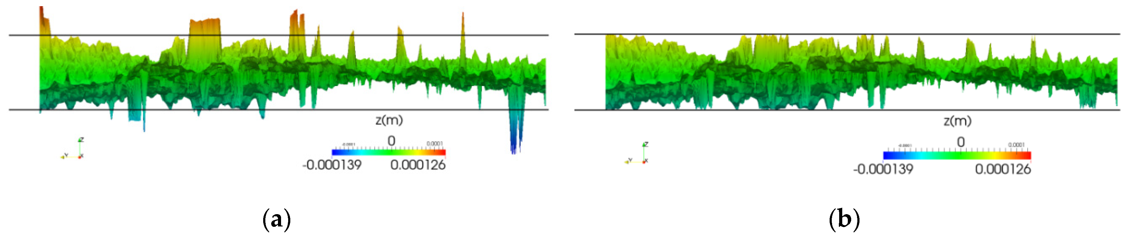
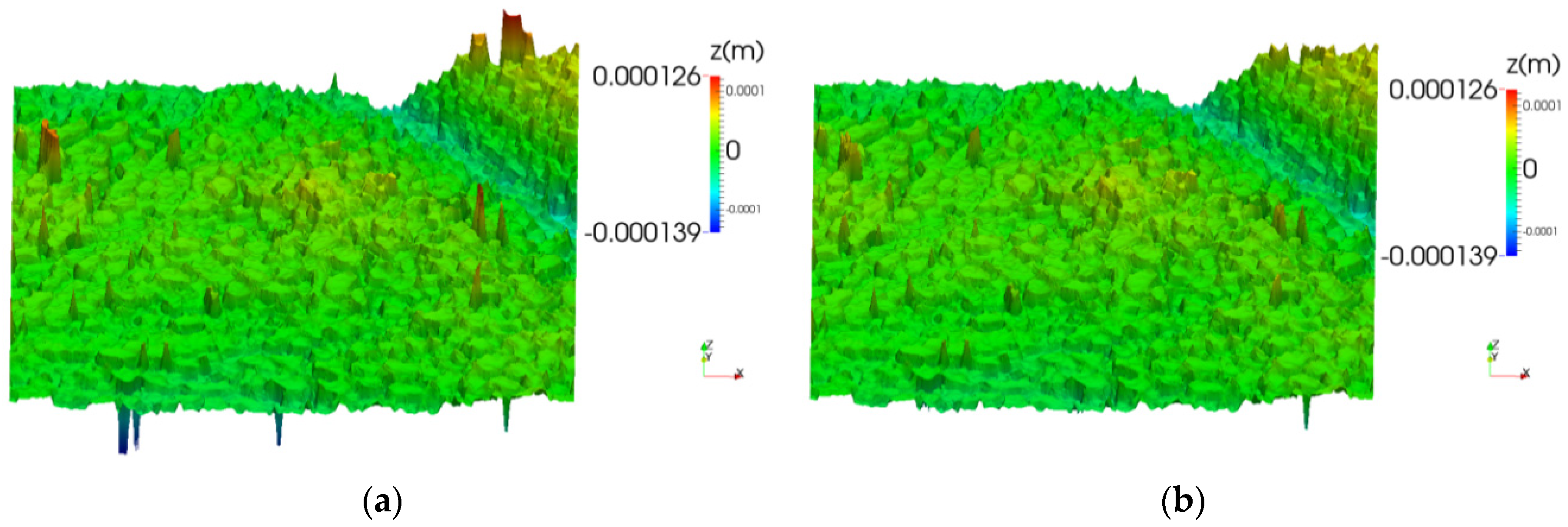
To demonstrate the applicability of SPH in simulating hydrodynamic lubrication with complex rough boundaries, a strip of a tomato leaf acquired using the confocal profilometer Leica DCM3D available in the MUSAM Lab of the Multiscale Analysis of Materials (MUSAM) research unit of the IMT School for Advanced Studies Lucca has been used as the lower boundary, see also the open data project Wiki Surface [
36]. This rigid tomato leaf is representative of a textured surface with geometrical complexity and roughness scale comparable with the artificial textures used to optimize linear sliders. Grid interpolator software [
37] has been used to elaborate the original tomato leaf surface as a grid-based data interpolator with modifications on the spatial resolution and the despiking procedure, as described in the following
Figure 1,
Figure 2 and
Figure 3.
Values greater than a positive threshold or smaller than a negative threshold have been discarded, being considered out-layers affected by profilometer measurement errors. The thresholds are provided as input data in terms of normalized variables. The upper threshold is
tu =
mz +
ntu·
σz, where
mz (m) is the average height,
σz = 1.81 × 10
−5 m the height standard deviation and
ntu = 3.5 a non-dimensional input factor. Analogously, the lower threshold is
tl =
mz −
ntu·
σz, with
ntl = 3.5. The interpolation influence radius provided as an input normalized influence radius (
rin = 10). A Shepard interpolation has been carried out, with the distance exponent provided as an input datum (
ed = 6). The despiking procedure described above allows the outliers of the raw surface to be filtered (
Figure 2 and
Figure 3).
For the CFD simulation, the initial fluid velocity
uf,0 (m/s) has been set as the average velocity of the solid plates. As the lower plate is still, then
uf,0 =
us,1/2, where “
s,1” denotes the upper plate. The reference velocity
U* =
us,1 = 50 m/s determines a Reynolds number (
Re = ca. 100) which guarantees a laminar regime within most of the bearing film (far enough from the mobile plate edges and the roughness elements). Omitting gravity is equivalent and alternative to replacing pressure with the reduced pressure (i.e., the difference between pressure and its hydrostatic component). The domain is laterally confined by vertical solid walls, where a boundary treatment scheme is applied [
23].
The domain length and width selected for the simulation were Ldom = 8.48 × 10⁻⁴ m and Wdom = 4.2 × 10⁻⁵ m, respectively. The domain depth is Hdom = 9.5 × 10⁻⁵ m. The slider length was L = 4.24 × 10⁻⁴ m. The initial position of the plate barycentre was represented by the horizontal coordinates xCM,0 = 0.35·Ldom = 2.968 × 10⁻⁴ m, yCM,0 = Wdom/2 = 2.1 × 10⁻⁵ m. The above length scales are chosen to impose that the sliding lasts enough to dynamically establish stationary conditions, to reproduce all the roughness elements of the fixed plate, the fluid film and the mobile plate, and to avoid useless computational demand. The upper plate inclination (with respect to the horizontal) is expressed by the slope angle α = 9.91 × 10⁻³ rad (0.568°). The dynamic viscosity of the fluid is µ = 319 × 10−3 Pa·s, representative of the motor oil “SAE 40” at ambient conditions, being the oil density equal to ρ = 900 kg/m3. This lubricant is still before the sliding of the mobile upper plate over the fixed plate of the bearing. The upstream and downstream fluid frontiers were modelled as open boundaries. The vertical and longitudinal monitoring lines for the profiles were located along the domain centreline (y = Wdom/2).
The spatial resolution for the present problem is defined by dx = 1.6 × 10⁻⁶ m, hSPH/dx = 1.3 and dx/dxs = 2, where hSPH is the SPH influence length, dx is the spatial resolution, the subscripts “f” and “s” represent the fluid and solid SPH particles, respectively.
Results are reported in terms of non-dimensional quantities for pressure
p (Pa), velocity magnitude and time
t (s):
where
p* is defined as normalized pressure and
h0 (m) is the representative oil depth (here equal to its minimum value), with
h0/
L = 1/25
L represents the upper plate length and
h0 is the minimum non-null value of
h—i.e., the mobile upper plate and the rough bottom plate are never in direct contact):
with the upper plate width equal to the domain width.
The following results refers to the final time step, which is equal to the physical time and representative of stationary conditions (T = 16.9, i.e., t = 3.00 × 10⁻⁶ s). Considering both the extremely small ratios of the involved length scales and the temporary unavailability of the best machine architecture usually adopted by the code, the simulation lasted 23.4 h on 68 cores Intel Xeon Phi7250 (Knight Landings, Intel, Santa Clara, CA, USA) at 1.4 GHz.
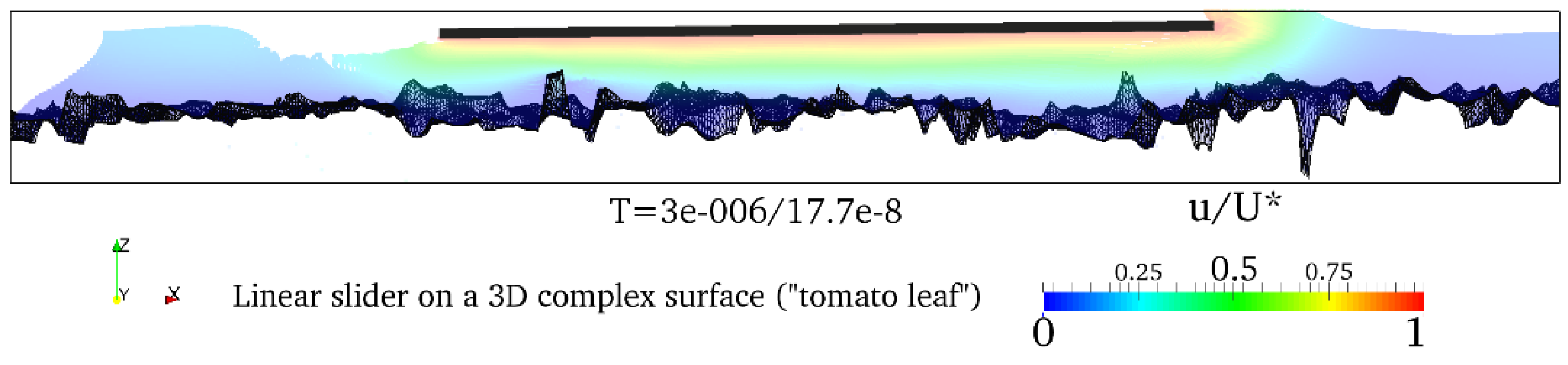
Figure 4 shows a lateral view of a representative 3D field of the
x-component of the normalized velocity. No-slip conditions are well reproduced at both the fixed frontier and the plate bottom. Within the confined fluid area, the velocity horizontal gradient depends on the local oil depth and the proximity to the edges of the mobile plate.
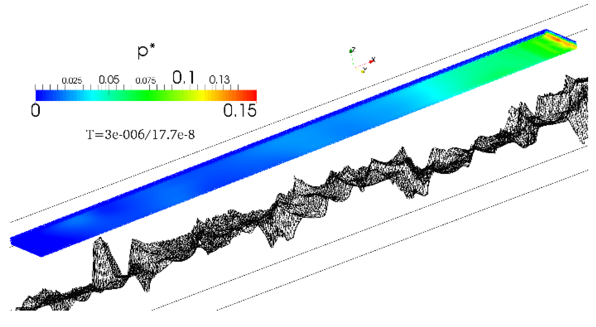
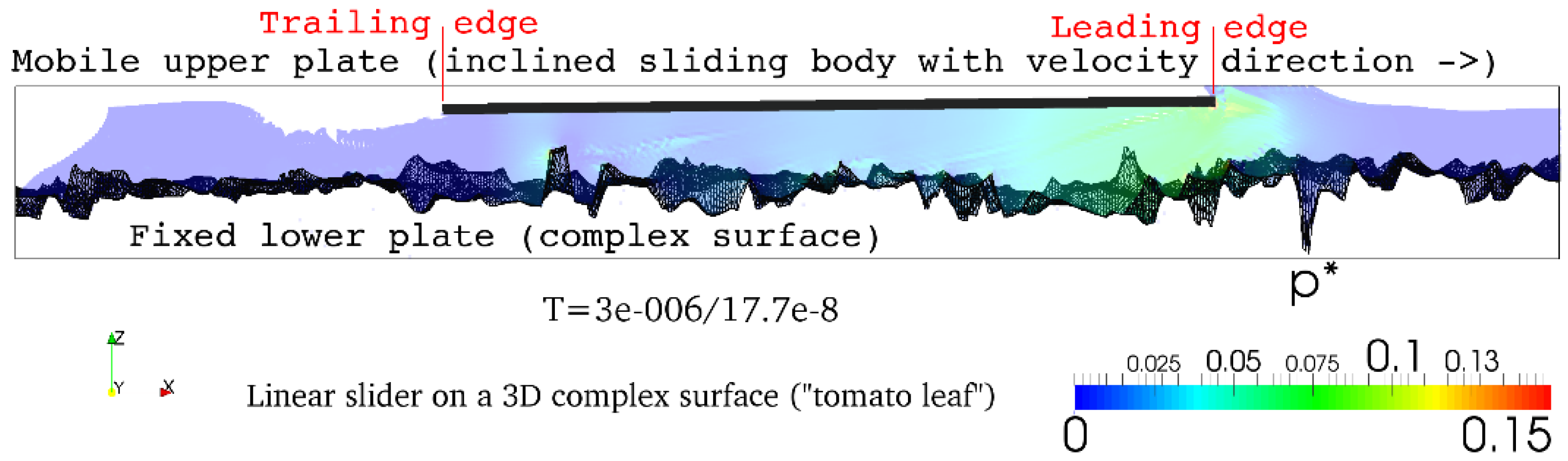
Figure 5 reports a representative lateral view of the 3D field of the normalized pressure. The leading edge and the trailing edge are locally featured by an over-pressure stagnation region and an under-pressure zone, respectively. The normalized pressure field is strongly perturbed by the asperities of the bottom complex surface.
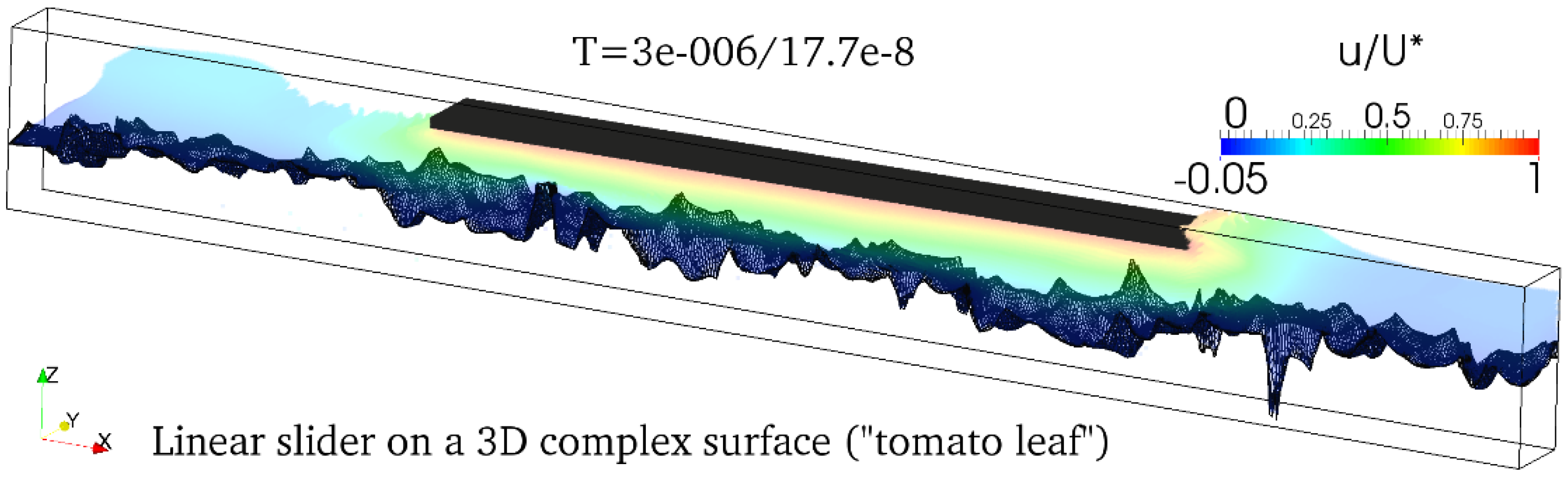
Figure 6 shows a representative 3D view of the field of the
x-component of the normalized velocity. The 3D effects (dependence on the
y-coordinate), due to the complex shape of the bottom surface, are relevant. The field of the
y-component of the normalized velocity is not reported because it is negligible (with respect to the
x-component) since the stationary regime is achieved.
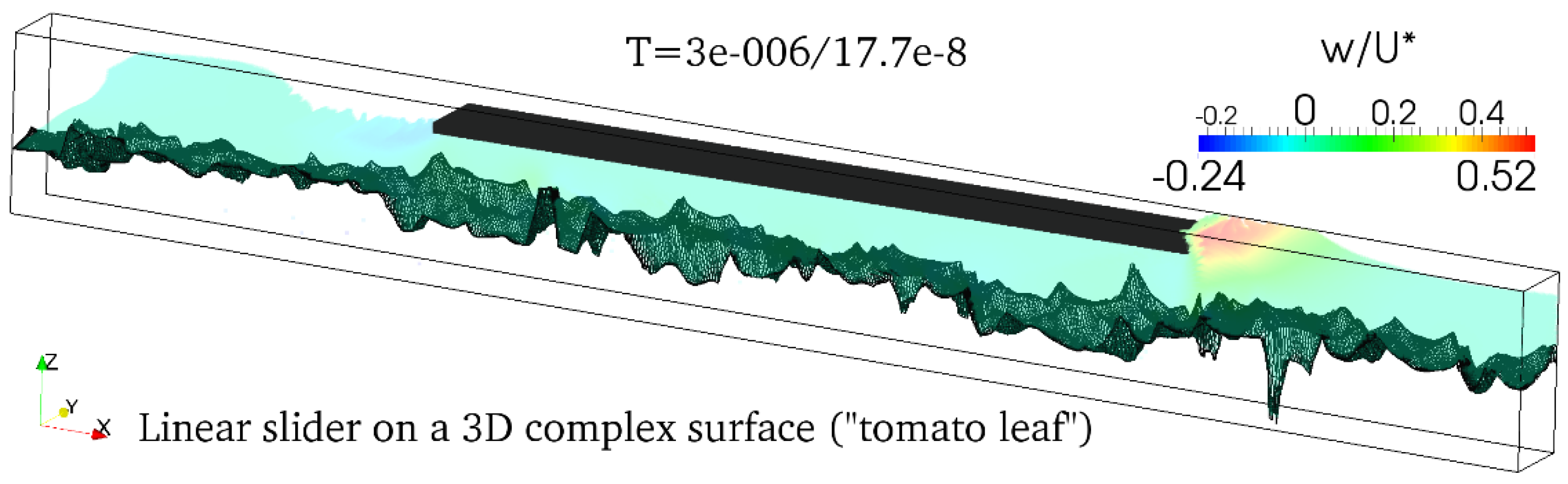
Figure 7 shows a representative 3D view of the field of the
z-component of the normalized velocity. The absolute value of the biggest positive value is 50% of the velocity scale and occurs at the leading edge. The absolute value of the smallest negative value is 24% of the velocity scale and occurs at the trailing edge.
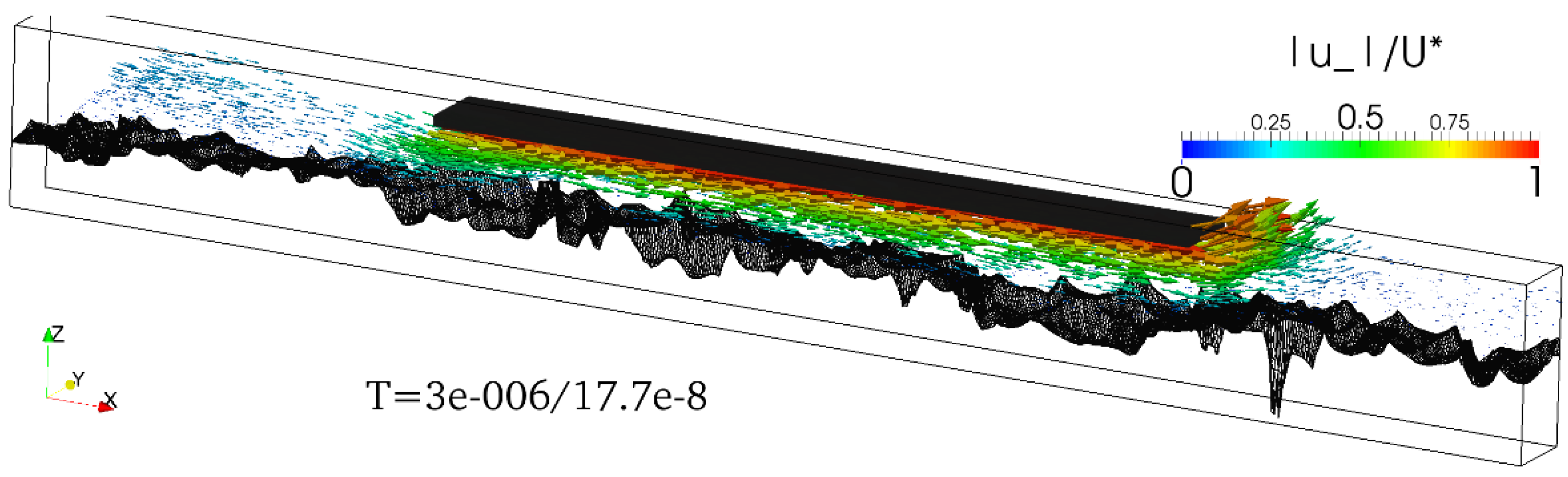
Figure 8 reports a representative 3D view of the normalized velocity both in terms of vector field and scalar absolute value. This example image integrates the information coming from the three velocity components simulated all over the fluid domain and demonstrates the importance of simulating the vertical component of the velocity vector, especially near the leading and trailing edges of the mobile plate.
Figure 9 reports a representative 3D view of the normalized pressure field at the interface between the oil and the upper plate. The presence of a complex 3D bottom surface introduces local fluctuations of the pressure field along the
x-axis as local perturbations to the parabolic shape of the pressure longitudinal profiles (Figure 11a): at the micro-scale the roughness elements represent obstacles featured by stagnation zones on the upstream faces and under-pressure regions on the downstream faces.
Comparing
Figure 4,
Figure 5,
Figure 6,
Figure 7,
Figure 8 and
Figure 9, one notices that the 3D effects are mitigated with
z. By contrast with the codes based on the simplified Reynolds’ equation for fluid films, this SPH code can represent the time and space evolution of the velocity vector, not just the stationary regime for the
x-component of velocity.
The simulation reference system is defined by the axis orientation of
Figure 4 and
Figure 6 (with the origin located at the lower left corner in the plan view—i.e., non-null values are used for the horizontal coordinates
x and
y−). At the same time, in order to monitor the simulated profiles, a local reference system is assumed with non-dimensional spatial coordinates, as explained below.
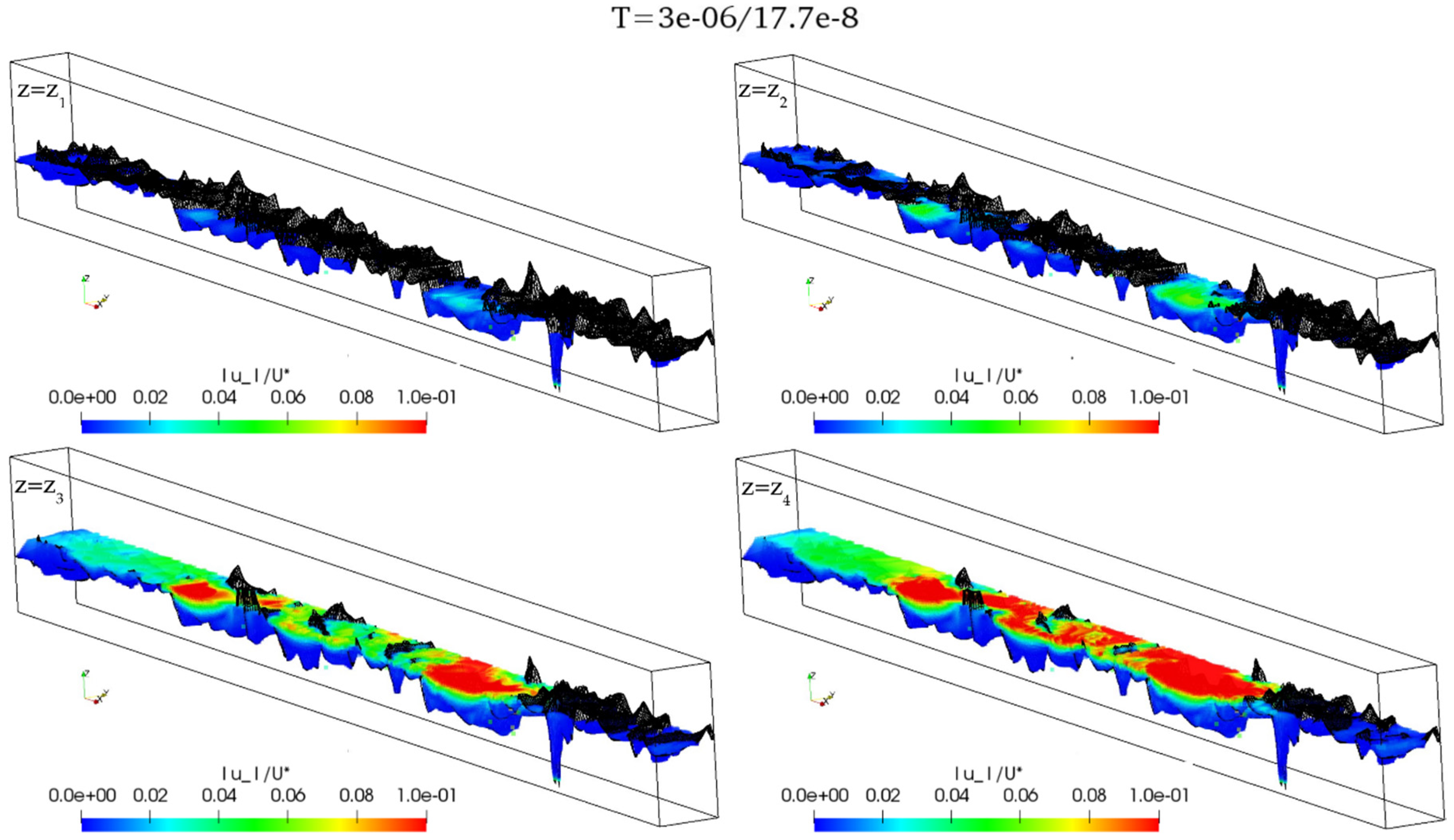
Figure 10 shows the projection of the absolute value of the non-dimensional 3D velocity field on different planes parallel to the flow direction at different heights
z. On these planes, the components of the 3D velocity vector field are characterized by a significant inhomogeneity along each one of the three directions aligned with the Cartesian axes. It is observed that as the
z coordinate increases, the velocity field along the corresponding plane is more affected by the velocity of the upper mobile plate.
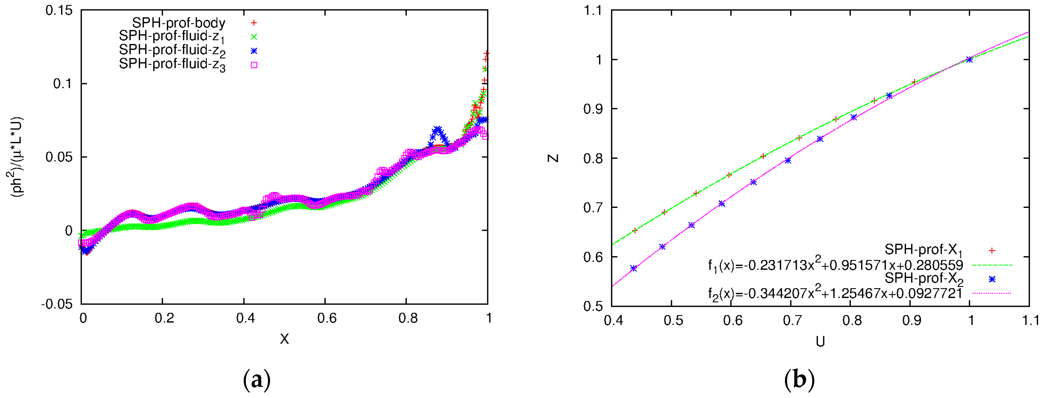
Figure 11a reports the normalized pressure longitudinal profile, from the inlet section (leading edge,
X = 1) to the outlet section (trailing edge,
X = 0) of the slider. Within these sections, the 2D pressure field is not imposed, but dynamically simulated until stationary conditions are achieved. The pressure field at the reference plot refers to the surface body particles representing the fluid–body interface (inclined monitoring line). The other three plots are monitored within the fluid domain at different non-dimensional heights
Z = (
z −
zbot)/
h:
Z1 = 1,
Z2 = 0.5,
Z3 = 0 (horizontal monitoring lines;
zbot is the local height of the lower plate). Results are plotted only within the bearing region (i.e., the portion of the fluid film laying between the upper plate and the bottom). The higher the position of the monitoring line (far from the asperities of the complex surface) the smoother the normalized pressure profile is. The two upper profiles are affected by a more pronounced estimation in the normalized pressure maxima at the leading edge. These two profiles provide very close results: some discrepancies are visible around the leading edge where the relative distance of these monitoring lines is maximum. By contrast with the analytical solutions (e.g., [
6]) and the codes based on the simplified Reynolds’ equation for fluid films, this SPH code can simulate non-null vertical gradients of the pressure field (as in [
38]), it takes into account the inertial effects due to the fluid-structure interactions at the leading and the trailing edges, and the profile concavity is directed upward.
Figure 11b shows two vertical profiles of the
x-component of the normalized velocity. The numerical probes are located at
X1 = 0.74 and
X2 = 0.98, where
X is the non-dimensional distance from the trailing edge (
x − x0)/
L and
x0 (m) is the
x coordinate of the trailing edge of the upper mobile plate at a fixed time. The concavity of the parabolic profile (directed downwards) increases as long as the monitoring position is located at a further distance from the leading edge. This feature is similar to what happens for a linear slider bearing over a flat bottom surface, where analytical solutions do apply. However, by contrast with the analytical solutions and the codes based on the simplified Reynolds’ equation for fluid films, the concavity of the velocity profile close to the leading edge is directed downward. As for linear sliders over a flat bottom (and the results from Reynolds’ equations for fluid films), the vertical profile of the horizontal velocity is quadratic in
z and it depends on
x.
As the spatial discretization of the numerical pressure profile is uniform, the numerical non-dimensional load-bearing capacity
LC is estimated as the average of the normalized pressure values over the mobile plate bottom (the squared parentheses represent an SPH estimation):
where
N represents the number of surface body particles along the centreline of the mobile plate bottom. The estimated non-dimensional load-bearing capacity for the above simulation is
LC = 0.026.


