Lubrication Regime Classification of Hydrodynamic Journal Bearings by Machine Learning Using Torque Data

Abstract

Hydrodynamic journal bearings are used within a wide range of machines, such as combustion engines, gas turbines, or wind turbines. For a safe operation, awareness of the lubrication regime, in which the bearing is currently operating, is of great importance. In the current study, highspeed data signals of a torque sensor, sampled with a frequency of 1000 hz in a time range of 2.5 s, obtained on a journal bearing test-rig under various operating conditions, are used to train machine learning models, such as neural networks and logistic regression. Results indicate that a fast Fourier transform (fft) of the highspeed torque signals enables accurate predictions of lubrication regimes. The trained models are analysed in order to identify distinctive frequencies for the respective lubrication regime.

1. Introduction

Hydrodynamic journal bearings are an important part of various machinery components due to their excellent damping, usability at high speeds and their straightforward setup. Especially in combustion engines, which are widely used in automotive, marine and energy industries, journal bearings are a key component for the functionality of these systems [1,2]. The failing mechanisms of journal bearings are well understood and often connected with seizure, which leads to a rapid fault, wear, fatigue or overheating. State-of-the-art journal bearings are composed of heterogeneous materials in order do fulfil demands depending on the area in which they are used [3,4]. Lubrication regimes, which are classified into boundary, mixed and fluid lubrication, are paramount to the current condition of a journal bearing system and to carry out predictions regarding wear, friction and failure likelihood. In any machinery equipment rapid failure of the system should be avoided, in order to guarantee a safe and cost efficient operation [5]. Failures in machine elements can in many cases be linked to an altered system behaviour, which can be measured with specialised measurement equipment. Consequently, many endeavours have already been carried out in order to develop systems which are capable of determining the current operation state of tribosystems, such as rolling element bearings or gears, and their likelihood for failure [6,7,8,9,10]. In rotating machinery applications the usage of vibration and acoustic emission sensors is common, since they can be integrated into the system relatively easy. In the case of acoustic emissions noise contamination is an issue, since these sensors do not only measure the energy of elastic waves released due to contact phenomena, but also the noise of surroundings, such as motors, cooling and actuation systems. Nevertheless, it has been proven that wear and frictional phenomena can be measured with acoustic emission technology [11,12,13,14]. Naturally, these sensors deliver time series data, which is usually processed to statistical scalar values, such as mean value, standard deviation, root mean square (RMS), or skewness. The magnitude of these values can be used in order to detect characteristics of the tribosystems [15]. Another approach is to perform angle synchronous averaging (ASA), which delivers values for a certain position range of the rotating machinery component [16,17]. Distinctive features in the signal can then be detected in the case of a faulty element in the system. Also, a common approach is the transformation of the time series into the frequency domain. Due to its speed and simplicity, the fast Fourier transform (fft) is widely used in the area of condition monitoring. However, since, in many cases, transient signals are monitored, methods better suited for this task, such as Wavelet analysis [18], are also very common. These tools are capable of detecting time-dependent events in the signal, since they also calculate the frequency intensity over time. Nevertheless, the calculation of Wavelet transforms takes considerably more effort compared to a fft.

Modern condition monitoring methodologies are mostly employed in rolling element bearings and gears. Faults in these components can already be detected reliably due to distinctive frequencies triggered by faulty elements within in the system. However, in the area of journal bearings it is less clear how different contact, lubrication, or wear scenarios influence the frequency range of measured data. Nevertheless, some authors already performed studies regarding the tribological state of journal bearings [15,19,20,21].

The goal of the present study is to use torque signals, which were measured regularly during testing, with a sampling frequency of 1000 hz and use them as an input for machine learning methods, namely artificial neural networks and logistic regression, in order to predict lubrication regimes. Torque sensors deliver reliable data since no contamination by surroundings is to be expected. Furthermore, in many applications torque signals are available out of the box, such as when using electric motors. In terms of complexity of the employed methods, a simplistic approach was chosen in order to enable a transfer of the methodology to actual industry applications.

2. Materials and Methods

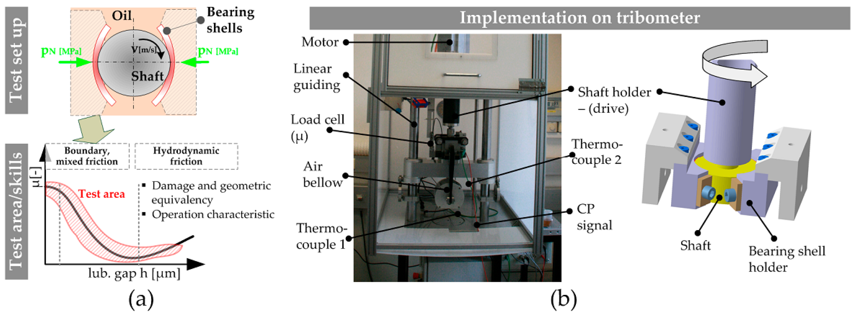
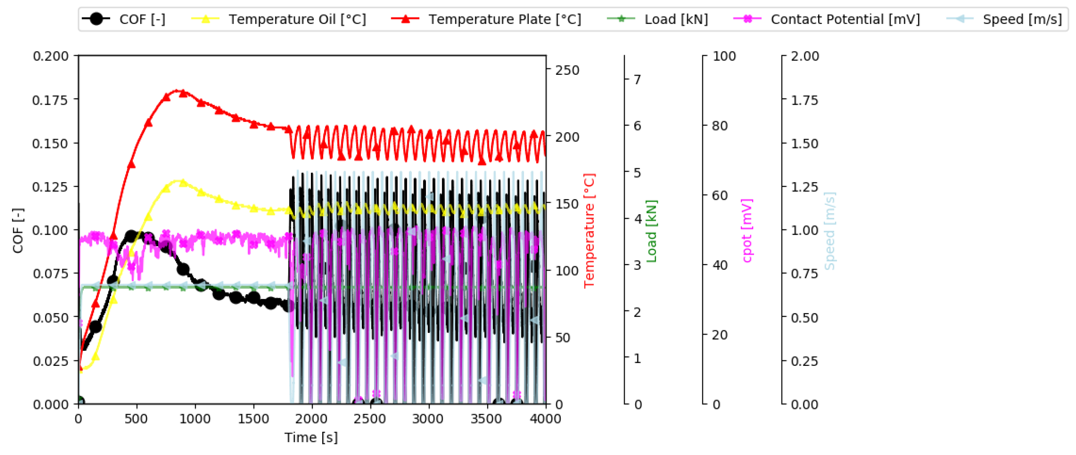
2.1. Experimental Setup

The test-rig which was employed for this study is based on a customised Phoenix Tribology TE92HS tribometer. Two journal bearing shells, which are also used in actual machinery components, are loaded radially against a cylindric steel specimen, which mimics the shaft. Therefore, equivalency to actual industry applications (automotive) can be achieved in terms of contact geometry, damage and operation characteristic, which is elucidated in Figure 1a.

In Figure 1b, the mechanical composition of the test-rig in bearing testing configuration is illustrated by means of a photograph and a 3D CAD drawing. There, the position of several sensors which deliver data regarding processes taking place in the tribosystem, is indicated. Two type-K thermocouples measure the temperature of oil-bath and bearing back-side. The load is induced symmetrically into the system via an air bellow. The torque measurement is realised by the load cell positioned on the left side of the test cell. Since the oil-containment is pivot mounted on an axial bearing, whereby the rotational axis is coinciding with the shaft axis, the torque can be calculated by taking into account bearing diameter and the distance between axis and load cell. This setup allows a direct measurement of forces taking place in the tribosystem and is not subjected to parasitic forces stemming from the rolling element bearings or seals of the motor shaft. Furthermore, an electric contact potential (CP) measurement systems, which allows a judgement of the current lubrication state, is available. The oil-bath was warmed to the set temperature with heating elements positioned within the oil containment. There was only free convection.

The nominal load of the torque load cell (Phoenix Tribology) is between 0 and 200 N. Since the sensor is based on strain gauge technology, the static error band is in the range of 0.2% of the maximum load, therefore the absolute tolerance is 0.4 N. The measured friction forces are in the range of 20–100 N, depending on the lubrication state. Thus the error introduced into the COF is in the range of 2% to 0.4%. Influences regarding the testing system, such as specimen manufacturing tolerances, oil batch homogeneity, or test-rig influences, trigger higher errors and are thus the limiting issue regarding testing accuracy and reproducibility, which has been shown in previous work by the authors [23].

For the data acquisition the software Compend (Phoenix Tribology), which runs on a standard Windows operating system was used. A slim device, which is integrated in the test-rig, contains all measurement amplifiers and transfers the data to the Windows PC via a serial bus.

Further details regarding this test-rig can be found in the respective publications [22,24].

2.2. Testing Procedure

All data was generated from test types with material combinations, consisting of bearing and shaft material, and test parameters as depicted in

Table 1. Test types with respective materials and parameters used for testing.

ID	Material Combination	Load	Maximum Speed	Oil Temperature
1	Aluminium-Steel	0.7 MPa	17 hz	65 °C
2	Lead-Steel	0.7 MPa	17 hz	65 °C
3	Polymer-Steel	0.7 MPa; 2 MPa	17 hz	65 °C
4	DLC-Steel	26.65 MPa	15 hz	145 °C

, whereby the load is specified with regard to the projected area of the bearing. All tests were carried out as Stribeck experiments, meaning that the specimen speed was continuously varied from 0 to a specified maximum speed. Therefore, depending on load, oil viscosity and specimen geometry, all lubrication regimes can be examined.

The bearing dimensions of diameter, shell thickness and clearance were 48.6 mm, 2 mm and 1.6 × ${10}^{-3}$, respectively, for aluminium, lead and polymer bearings and 26 mm, 3 mm and 1 $\times {10}^{-3}$ for the DLC-steel material combination. For all experiments oils with a 5W30 viscosity grade were used.

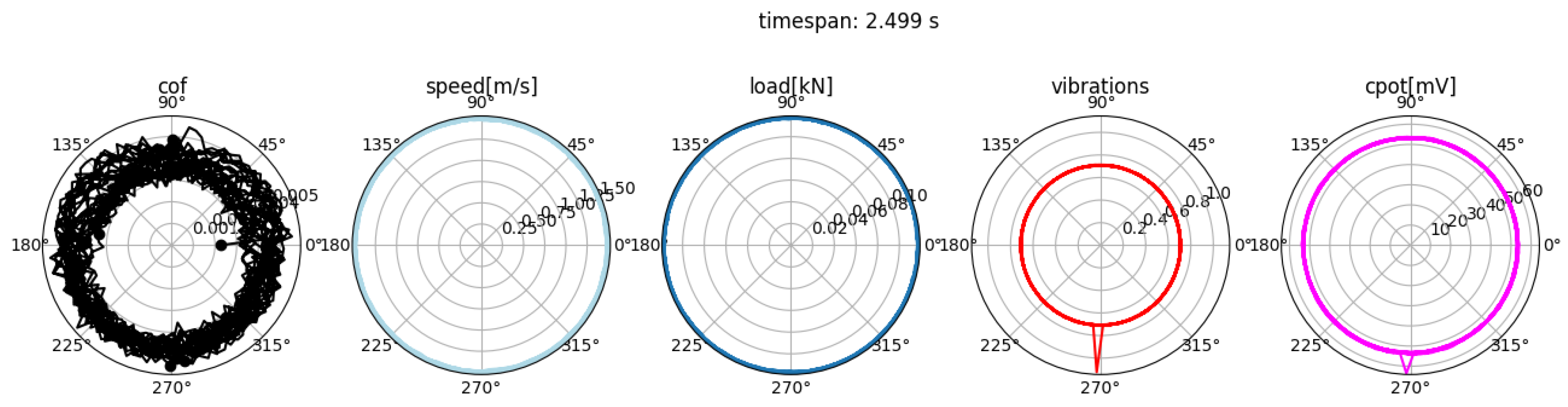
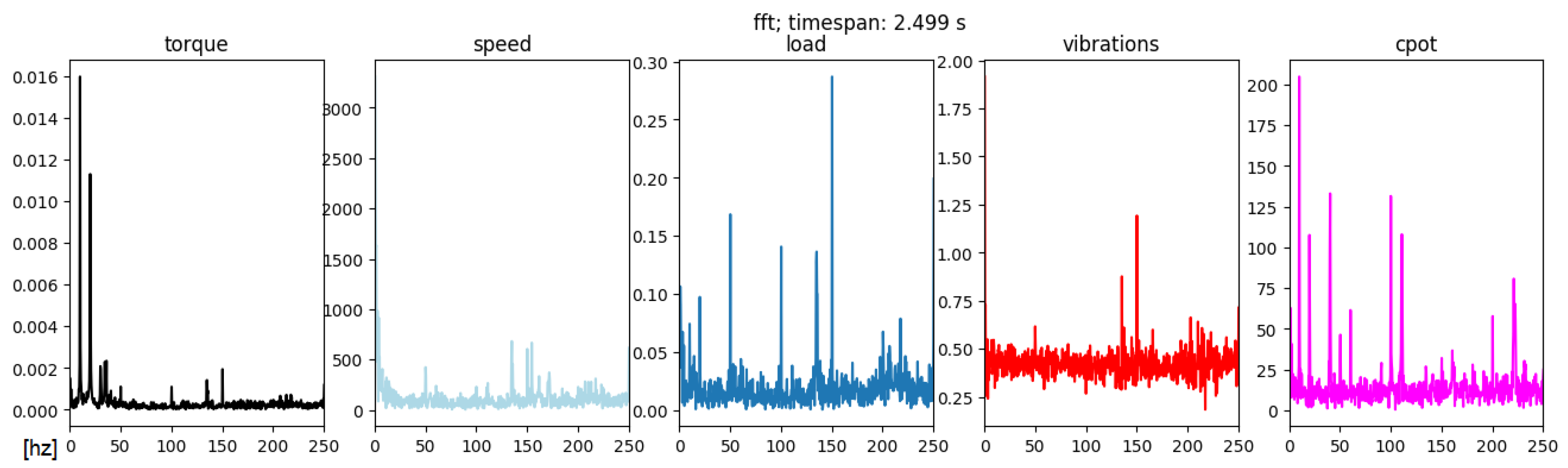
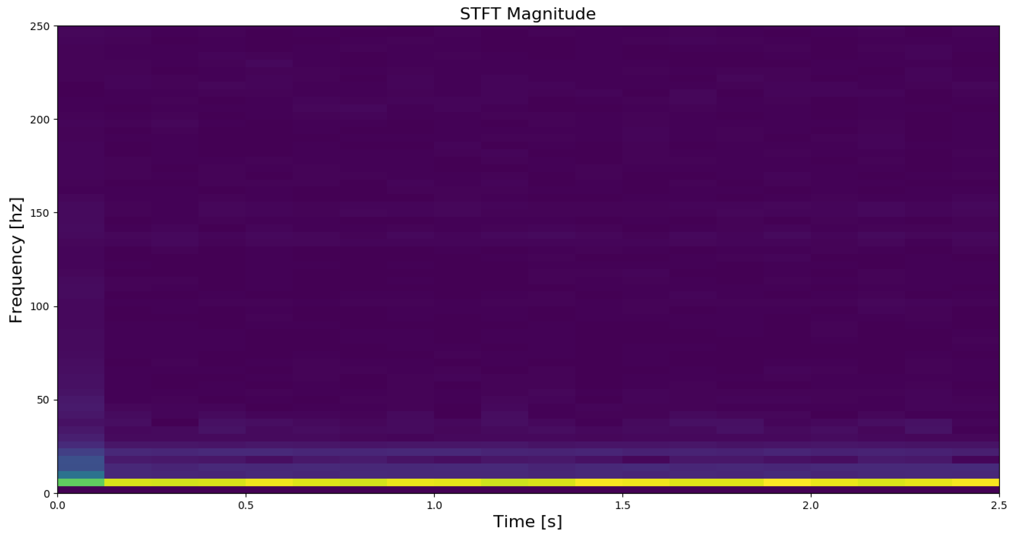
2.3. Data Processing

All data generated by the sensors of the test-rig is, on the one hand, stored with a frequency of 10 hz, which is denoted as low-speed data. On the other hand, selected sensors (torque, speed, load, vibration, contact potential) with enhanced capabilities, are operated with 1000 hz. The data resulting is referred to as high-speed measurements from here on. In order to simplify the interpretation of results, the angular position of the shaft is calculated based on the speed signal according to:

$$\varphi ={\varphi }_0+{\int }_{t_0}^t\omega dt$$

(1)

Therefore, for each time record a respective position of the shaft can be stated, improving the readability of the measured data by using polar plots. Since the high-speed data is not angle synchronous, discrete Fourier transforms of the signals are carried out in order to transfer the signals from time to frequency domain:

$$X_n=\sum _{n=0}^{N-1}{x}_n{e}^{-i2\pi kn/N}$$

(2)

Note that in this equation i corresponds to the imaginary unit and the indexes n and k are used for summation. By taking into account symmetries the fft reduces the operations required to calculate the discrete Fourier transform from $\mathcal{O}\left(N^2\right)$ to $\mathcal{O}\left(NlogN\right)$ [25]. Therefore, an online calculation of fft spectra becomes feasible and can be carried out directly after the respective high-speed measurement.

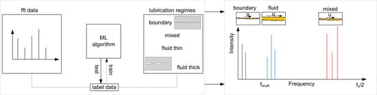
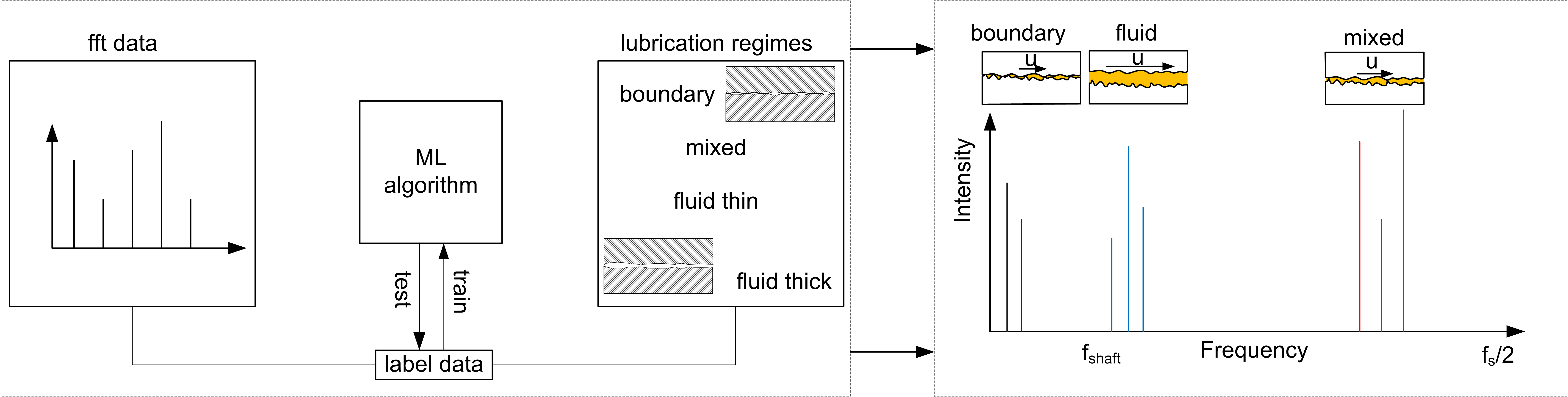
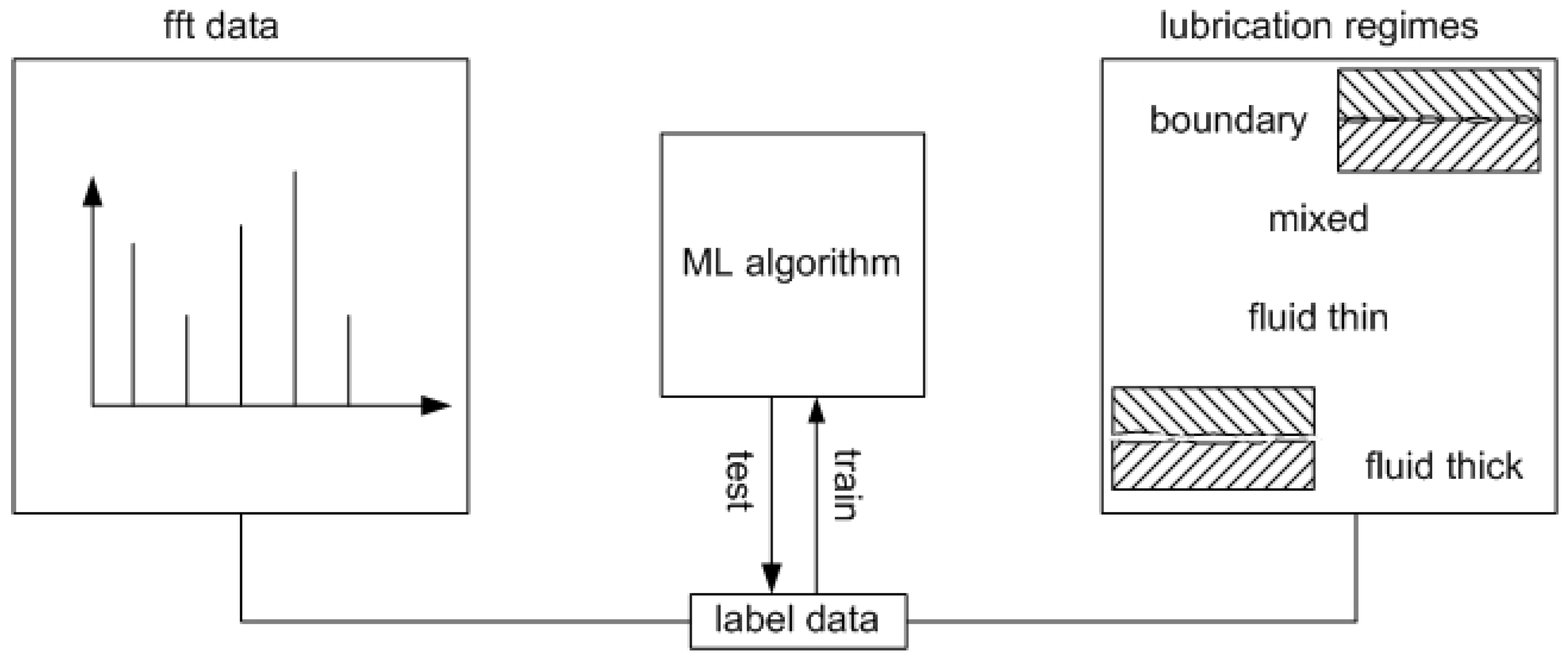
2.4. Machine Learning Methods

The basic idea of machine learning is, instead of coding hard rules which then predict a lubrication regime for a specific signal, to use data for training an algorithm. Figure 2 illustrates the approach based on the context of this article.

The fft signals based on the high-speed torque measurements are labelled manually as boundary (0), mixed (1), fluid thin (2), or fluid thick (3)—these targets are mutually exclusive, meaning that one fft signal can only be attributed to exactly one lubrication regime. Since human interference is required, this approach belongs to supervised machine learning methods. The data is then organised according to standard machine learning conventions. The ffts are stored in the matrix X, which is of dimension $[m\times n]$, whereby m describes the number of instances (signals in this case) and n the number of features (frequency range in this example). The label vector y of dimension $[m\times 1]$ contains the respective lubrication regime for each instance (signal). Independent of the actual learning algorithm employed, the following work-flow is maintained:

• Perform fft transform of torque high-speed data signals.
• Manually label each fft record to a lubrication regime.
• Shuffle all records to eliminate order influence.
• Scale data to improve convergence and accuracy of algorithms.
• Split the data into a training and a test set taking into account stratification.
• Train the model with a batch gradient descent algorithm.
• Evaluate performance on training and test set based on accuracy.

2.4.1. Logistic Regression

As part of this study, a logistic regression algorithm was employed for the classification of lubrication regimes since datasets were relatively small. This method works in a similar way to standard linear regression, except that a logistic function is applied to the product of x (which corresponds the one instance) and $\theta$, which is the weight vector of dimension $[n\times 1]$.

$$\widehat{p}=\sigma \left({\theta }^T\mathbf{x}\right)\sigma :[-\infty ,\infty ]\to [0,1]$$

(3)

The exact definition of the logistic function is as follows:

$$\sigma \left(t\right)=\frac{1}{1+e^{-t}}$$

(4)

Based on the evaluation of the logistic function a decision regarding the classification is then made according to:

$$\widehat{y}=\left\{\begin{array}{cc}0\hfill & \mathrm{if}\widehat{p}<0.5\hfill \\ 1\hfill & \mathrm{if}\widehat{p}\ge 0.5\hfill \end{array}\right.$$

(5)

While classical regression relies on the mean square error (MSE) as a cost function, a different approach is used for logistic regression. Based on the observation that negative logarithm of a number close to zero becomes very large, the following cost function is introduced:

$$J\left(\theta \right)=\frac{1}{m}\left[y^i(-log({\widehat{p}}^i))+(1-y^i)(-log(1-{\widehat{p}}^i))\right]$$

(6)

Consequently, a wrong classification is penalised accordingly for both cases, positive classification of a negative and negative classification of a positive. Based on this cost function a batch gradient descent algorithm is then used to find optimal values for the weight vector $\theta$, whereby $\eta$ is the learning rate and has to be specified according to the problem at hand.

$${\theta }_{i+1}={\theta }_i-\eta {\nabla }_{\theta }J\left(\theta \right)$$

(7)

Since the current problem contains four different target classes a one-vs-rest (OvR) scheme is employed, which trains four separate classifiers for each lubrication regime.

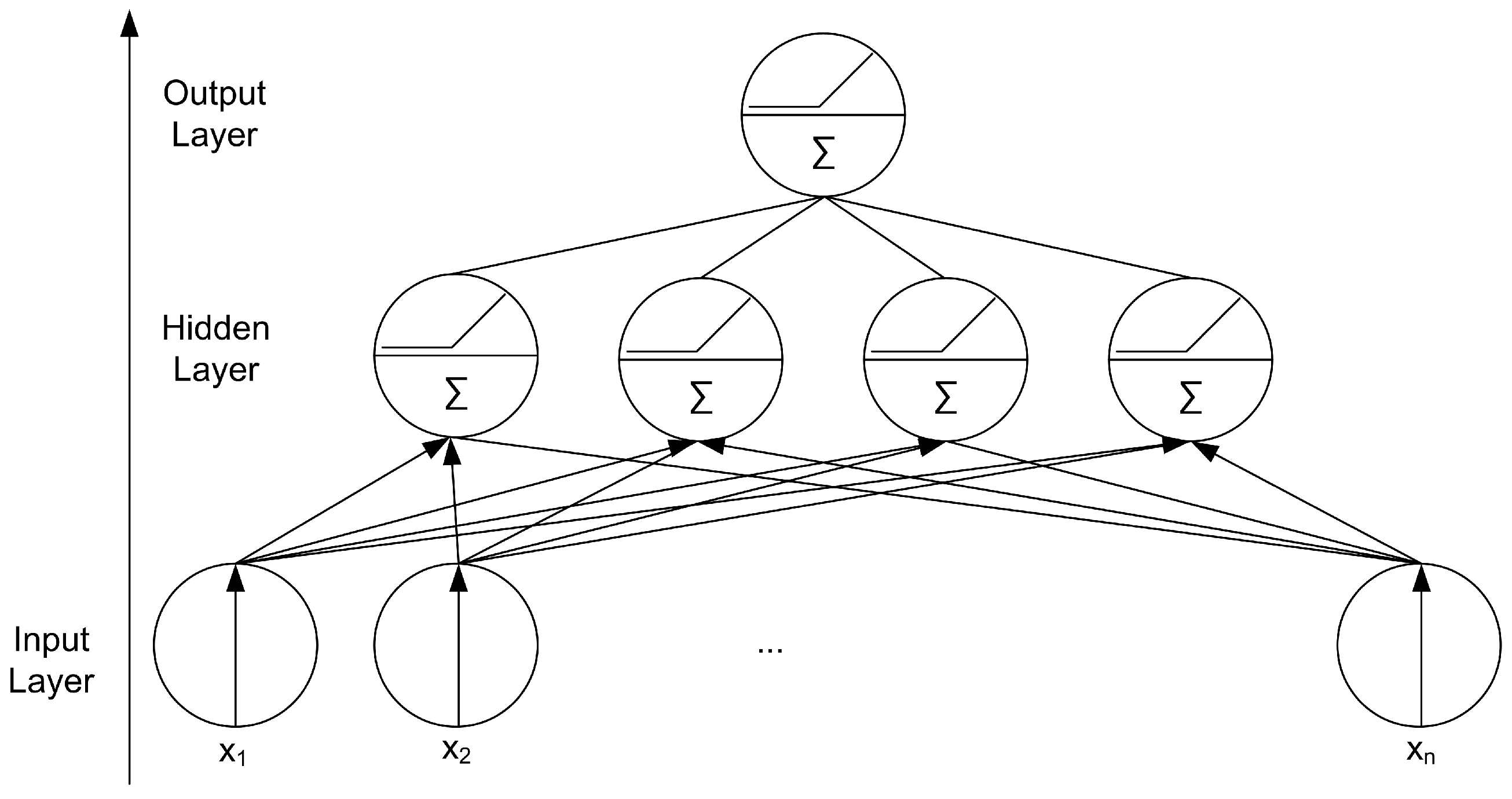
2.4.2. Deep Neural Networks (DNNs)

Deep neural networks have become one of the most powerful methods for challenging tasks, such as image classification, speech recognition, or machinery fault detection. Basically, a neuron has an arbitrary number of inputs and then sends, depending on these inputs, exactly one output value. Neurons can be interconnected in order to tackle complicated problems, as depicted in an example in Figure 3. Each input value, as for example an intensity at a certain frequency, is connected to every neuron in the first hidden layer. All layers, including input, hidden and output can contain arbitrary numbers of neurons.

As indicated with the summation symbol in each neuron, a sum of all input values is calculated, whereby a different weight is employed for each input. The resulting scalar is then fed to an activation function, which can be chosen from several options. In this paper, rectified linear units (ReLUs) will be used due to their straightforward differentiability and non-saturating nature at high input values. The summation and activation of each neuron layer for a dataset X can be conveniently noted in matrix form as follows:

$$\mathbf{Y}=\mathrm{ReLU}\left(\mathbf{X}{\mathsf{\Theta }}^T\right)$$

(8)

In Figure 3, only one hidden layer is depicted, however, in practical applications up to a few hundred layers can be employed. Furthermore, the output layer can also contain an arbitrary number of neurons. In the current paper for instance, four different classes are available, consequently, a DNN with four output neurons will be employed. The values of the weights are optimised with the back-propagation algorithm, which calculates, based on errors of the output layers, the respective error contributions of each neuron. Based on these errors, the weights are then adjusted [26]. More detailed information regarding the machine learning methods used within the scope of this article can be found in respective literature [27,28,29].

3. Results

Figure 4 shows a characteristic test graph based on low-speed data measurements, which have been obtained with a frequency of 10 hz. In this test, the first 1800 s are used for heating the system to the desired oil temperature and running-in. Thereafter, Stribeck cycles are carried out which means, that the speed is gradually varied from zero to a specific value. The load is kept constant throughout the test. This type of graph is typically used for the tribological analysis of lab tests and can provide valuable information regarding processes taking place in the system. Within a time range of 500–1500 s, the COF is lowering continuously which is associated to an improving adaptation of the surfaces to each other. Also note the excellent reproducibility of the Stribeck cycles which are always yielding almost identical COF values.

Figure 5 depicts a detailed view in a range of 60 s of a Stribeck cycle. There, well known relationships, such as COF-speed or COF-CP, can be identified, which are key for characterising tribological systems. As the speed rises lubricant mass flow between bearings and shaft increases, which leads, due to hydrodynamic effects, to an increased load bearing capacity of the lubricant and consequently facilitates the build-up of a lubricant film between the involved components which reduces, as observed in Figure 5, the COF and lowers direct solid contacts. These effects are physically well justified and governed by the Reynolds equation, which is a special variant of the Navier–Stokes-equations. Details regarding the simulation of hydrodynamic friction can be found in respective publications [30,31,32].

Generally, the CP only allows binary judgement of the lubrication state, meaning that no reliable inference between film-thickness and CP can be made. Due to lubricant additives, which form non-conductive layers on surfaces, the CP can be non-zero at zero speed as well.

As often employed in statistical analysis the Pearson correlation coefficient can be calculated for two randomly distributed variables X and Y, whereby the term on the right describes correlation for a sample:

$${\rho }_{X,Y}=\frac{E\left[(X-{\mu }_X)(Y-{\mu }_Y)\right]}{{\sigma }_X{\sigma }_Y}=\frac{{\sum }_{i=1}^n(x_i-\overline{x})(y_i-\overline{y})}{{\sigma }_x{\sigma }_y}$$

(9)

This analysis was carried out for 6 selected variables, whereby correlation was calculated for all possible combinations, leading to the matrix depicted in Figure 6. Note that the correlation normalises dependence between −1 and +1.

The correlation matrix depicts well that the variables measured are not independent and provide a sound method to point out correlations of signals within tribological experiments. Nevertheless, the causality between variables has to be justified physically and therefore needs additional computational methods, such as fluid dynamics, heat transfer, or structural dynamics.

Based on the analysis of the low-speed data of the torque (COF) signal only, it is difficlt to classify lubrication regimes, and other data, in this case contact potential, is necessary for an elaborated judgement.

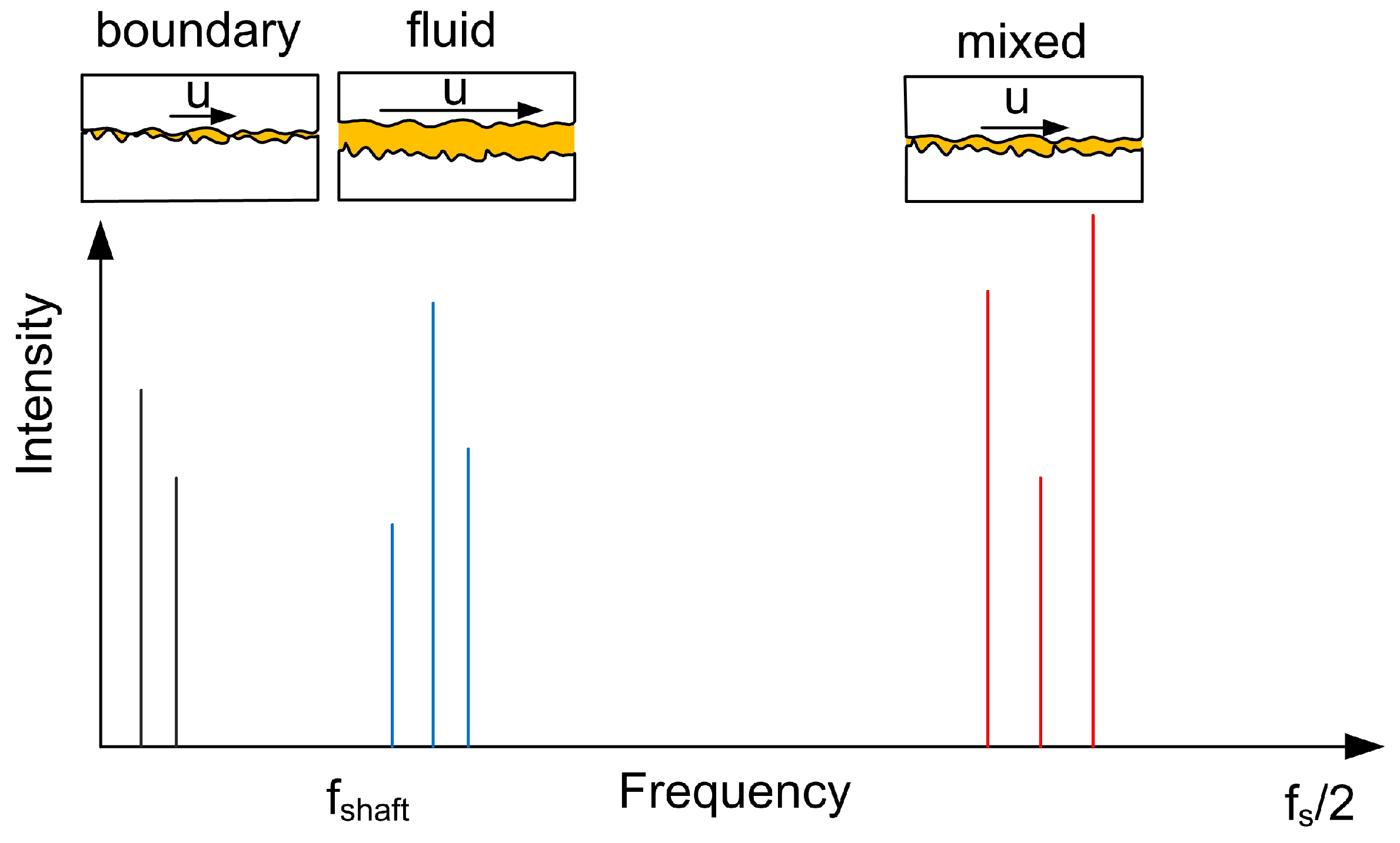
3.1. High-Speed Data Results

High-speed data measurements were carried out regularly during the tests for short periods of 2.5 s. In total 888 records from different experiments were used in this study, whereby signals were recorded in all lubrication regimes. Figure 7 shows one of these measurements, which was classified as fluid (thick) lubrication, based on the steady state contact potential.

The fft transformed signals corresponding to Figure 7 are shown in Figure 8. A frequency range from 0 to 250 hz is depicted since the intensity between 250 hz and 500 hz, which is in this case the Nyquist frequency, was negligible.

The transforms provide some distinctive areas, for example torque shows several peaks in the range between 25 hz and 50 hz. Nevertheless, it is very difficult and especially time consuming to go through every fft and to identify, depending on a specific lubrication regime, characteristic peaks and find physical legitimation for these. In this case machine learning methods can be of great value, since, by feeding them with high quality data, an automated detection of characteristic areas becomes feasible.

In order to investigate if the behaviour of the system was stationary within the measurement period, short time Fourier transforms (STFT) were carried out for selected samples. Figure 9 shows the STFT of the torque sample depicted in Figure 7 with a window size of 250 entries and an overlap of 125 data points.

The stationary behaviour of the signal can be confirmed, since the characteristic frequencies only vary slightly in terms of magnitude until about 0.1 s.

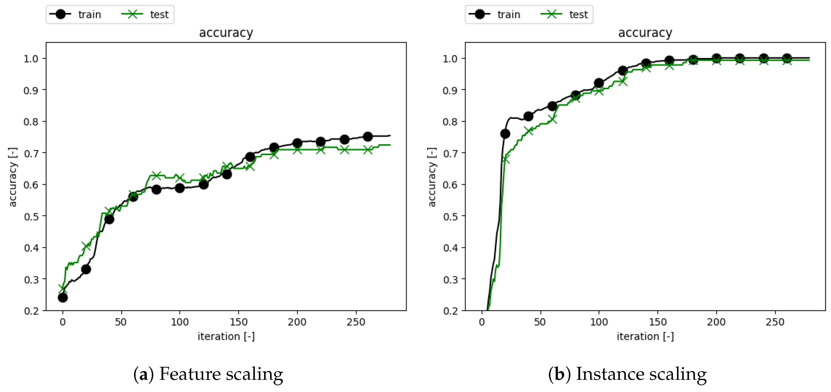
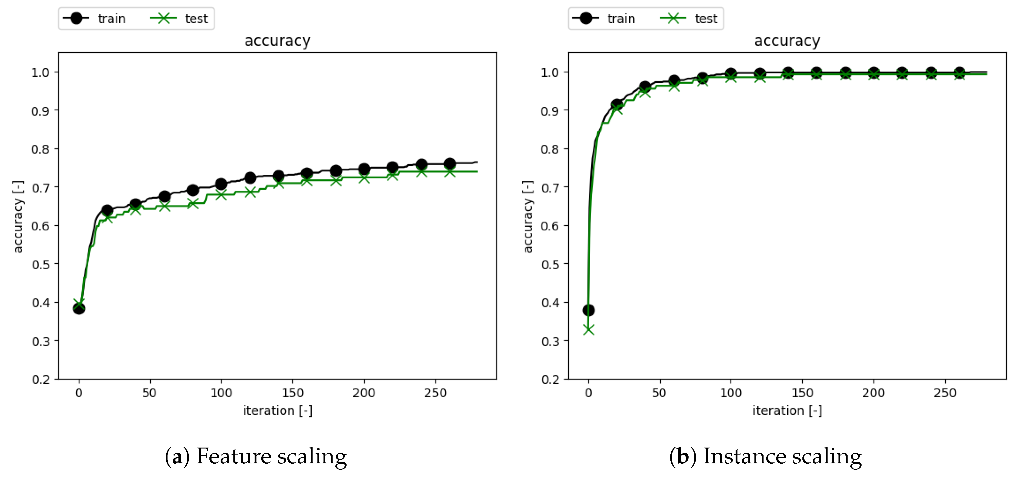
3.2. Classification Results

For the classification task only the torque ffts were used, since this kind of data is available in many practical applications as well. Due to the relatively small dataset consisting of 888 instances with 512 features each, a deep neural network with six hidden layers, containing 256, 128, 64, 32, 16 and 8 neurons, respectively, was investigated as a starting point. The dataset was shuffled and then split into training and testing sets, containing 80% and 20% of the instances, respectively. The library tensorflow [33] was used for building and computing the neural networks.

For the numerical experiments two different types of scaling have been employed. Firstly, a method commonly used in data analytics, where each feature is scaled, was employed:

$$X_{i,j}^{scaled}=\frac{X_{i,j}-\mathrm{mean}\left(X_{:,j}\right)}{\mathrm{std}\left(X_{:,j}\right)}$$

(10)

whereby i corresponds to the current instance and j to the current feature. Secondly, another option is to scale each instance, again with mean and standard deviation:

$$X_{i,j}^{scaled}=\frac{X_{i,j}-\mathrm{mean}\left(X_{i,:}\right)}{\mathrm{std}\left(X_{i,:}\right)}$$

(11)

Figure 10 depicts the accuracy of training and test sets for each iteration of the batch gradient descent algorithm with a learning rate of 0.01.

Feature scaling is very commonly used in classical data analysis, however, for fft series it is not performing well, since characteristic peaks of series might vanish.

Based on the good accuracy achieved by this network, the hidden layers were gradually removed. Figure 11 presents the results of a shallow neural network with one hidden layer containing 32 neurons.

It can be concluded that even the shallow neural network achieves good results, which is an indicator that linear classifiers will also perform well for the dataset. Since the back-propagation algorithm has considerably less weights to optimise, convergence is achieved already in the area of 100 iterations.

To summarise the results obtained with DNNs, accuracies after 260 iterations are depicted in

Table 2. Accuracies of trained DNNs on the test set.

DNN	Scaling	Accuracy
Hidden 6	None	52.96%
Hidden 1	None	54.47%
Hidden 6	Feature	72.39%
Hidden 1	Feature	73.88%
Hidden 6	Instance	99.25%
Hidden 1	Instance	99.25%

. Note the inferior results for the cases when no scaling is applied.

As a further simplification the data was fed to a logistic regression model and trained with a gradient descent algorithm. The machine learning framework scikit-learn was used for these investigations [34], whereby the values for learning rate, tolerance and maximum iterations were set to 0.1, 1 $\times {10}^{-5}$ and 50, respectively. No regularisation was applied to the loss function $J\left(\theta \right)$. Indeed the logistic regression classifier also is capable of achieving high accuracies as highlighted in

Table 3. Accuracies of logistic regression models on the test set.

Scaling	Accuracy
None	73.03%
Feature	92.13%
Instance	99.25%

.

Instance scaling again yields the best results. The high accuracy indicates that the different classes are linearly separable in the dataset used for training the model.

4. Discussion

The numerical experiments presented in Figure 2 and Table 2 and Table 3 indicated, that a relatively simple neural network, containing only one hidden layer, and a logistic regression model are capable of predicting the respective lubrication regimes with high accuracy. Therefore, an analysis of the weights calculated by the models should highlight frequency areas, which lead to a classification of a specific lubrication regime. Consequently, the weights trained by a logistic regression model, are depicted in Figure 12. Since an OvR approach was used, four separate classifiers were trained, which means weights were calculated for each class for the whole frequency spectrum.

In Figure 12, it is interesting to see, that each class can be linked to distinctive frequencies. Class 1 (mixed lubrication) for instance, peaks at comparatively high frequencies of 210, 140 and 110 hz. This could be linked to transient contact phenomena triggered by waviness features of the surfaces or in general to surface roughness effects. Classes 2 and 3, which correspond to fluid lubrication, do not show positive peaks in the frequency range between 100 and 300 hz. Peaks rather occur around 10, 15, 20 and 30 hz, those frequencies are close to the specimen speed during the tests, which was between 0 and 17 hz. The fluid lubrication regime is characterised by an oil film, which separates both surfaces and has good damping properties. Consequently, the absence of high range frequencies is not surprising. An explanation for the dominant frequencies detected for this lubrication regime could be small surface defects on the specimens, which repeatedly enter the contact zone with frequencies related to the testing speed. Also, the test-rig itself, which is operated with a precisely manufactured spindle and high performance roller bearings, but nevertheless has imperfections, is a possible source of these frequencies. Additionally, a perfect alignment between shaft and journal bearings is practically not feasible, leading to inevitable contact imperfections. Lastly, the boundary friction regime, class 0, is characterised by an absence of any frequencies above 5 hz, which is a consequence of the low sliding speed and the resulting low frequency of surface roughness interactions. These findings are summarised schematically in Figure 13.

5. Conclusions

Within the presented study, 888 high-speed torque measurements taken from various experiments, which were carried out on a journal bearing test-rig, were classified regarding their lubrication regime. Machine learning methods were then trained on training data and their accuracy was evaluated on a test dataset. Regarding the classification task the following outcomes were found:

• Neural networks perform well on the classification task, reaching accuracies of up to 99.25%.
• A shallow neural networks performs equally well on the problem and reaches high accuracies after fewer iterations compared to a deep neural network.
• A linear classification model, namely logistic regression, also delivers the same quality of results compared to neural networks.
• Feature scaling, which is often used in data analysis, is not suitable for the task of fft classification, since characteristic peaks might disappear due to the process.
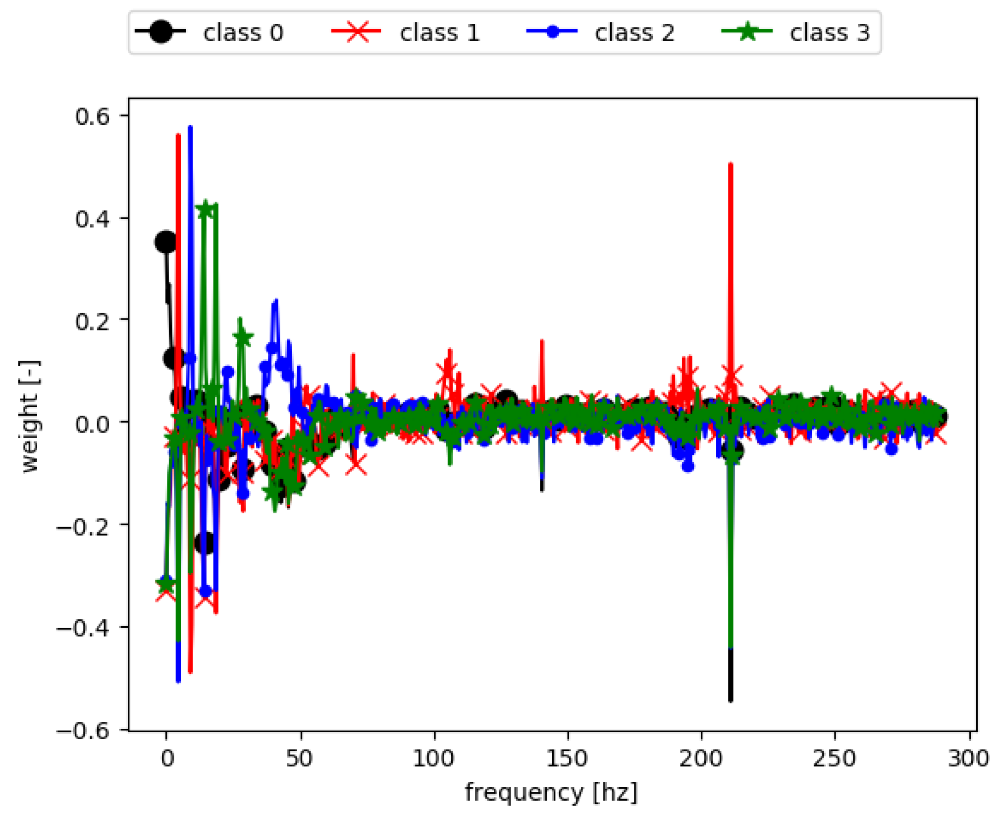
• Each lubrication regime yields characteristic frequencies, which could be linked to different phenomena, such as specimen waviness, imperfections, or test-rig influences.

The results of this study will serve as a foundation for further investigations regarding machine learning tasks of tribological experiments, as for example the classification of acoustic emission signals, which cover frequency ranges of up to 400 khz, and therefore provide a good candidate for an automated detection of characteristic frequencies. It can be expected that the presented methodology would also be applicable of revealing frequencies which are distinctive for different wear phenomena and their intensity. Since an application on all sorts of different measurement techniques, such as vibration or acoustic emission sensors, is possible, a wide range of different measurement setups can be investigated in order to predict tribological phenomena in industry applications which are using journal bearings.

References

1. Van Basshuysen, R.; Schäfer, F. Handbuch Verbrennungsmotor: Grundlagen, Komponenten, Systeme, Perspektiven; Springer: Berlin/Heidelberg, Germany, 2010. [Google Scholar]
2. Aufischer, R.; Hager, G.; Hamdard, K.; Offenbecher, M. Bearing Technology Combinations for Low Friction Cranktrains. MTZ Ind. 2016, 6, 56–63. [Google Scholar] [CrossRef]
3. Becker, E.P. Trends in tribological materials and engine technology. Tribol. Int. 2004, 37, 569–575. [Google Scholar] [CrossRef]
4. Grün, F.; Gódor, I.; Eichlseder, W. Fundamentals of optimizing aluminium-based journal bearing materials. Proc. Inst. Mech. Eng. Part J J. Eng. Tribol. 2009, 223, 777–785. [Google Scholar] [CrossRef]
5. Yang, W.; Tavner, P.J.; Crabtree, C.J.; Feng, Y.; Qiu, Y. Wind turbine condition monitoring: Technical and commercial challenges. Wind Energy 2014, 17, 673–693. [Google Scholar] [CrossRef]
6. McFadden, P.; Smith, J. Model for the vibration produced by a single point defect in a rolling element bearing. J. Sound Vib. 1984, 96, 69–82. [Google Scholar] [CrossRef]
7. Brie, D. Modelling of the spalled rolling element bearing vibration signal: An overview and some new results. Mech. Syst. Signal Process. 2000, 14, 353–369. [Google Scholar] [CrossRef]
8. Slavič, J.; Brković, A.; Boltežar, M. Typical bearing-fault rating using force measurements: Application to real data. J. Vib. Control 2011, 17, 2164–2174. [Google Scholar] [CrossRef]
9. Tandon, N.; Nakra, B.C. Comparison of vibration and acoustic measurement techniques for the condition monitoring of rolling element bearings. Tribol. Int. 1992, 25, 205–212. [Google Scholar] [CrossRef]
10. Castejón, C.; Lara, O.; García-Prada, J. Automated diagnosis of rolling bearings using MRA and neural networks. Mech. Syst. Signal Process. 2010, 24, 289–299. [Google Scholar] [CrossRef]
11. Boness, R.; McBride, S.; Sobczyk, M. Wear studies using acoustic emission techniques. Tribol. Int. 1990, 23, 291–295. [Google Scholar] [CrossRef]
12. Baccar, D.; Söffker, D. Wear detection by means of wavelet-based acoustic emission analysis. Mech. Syst. Signal Process. 2015, 60, 198–207. [Google Scholar] [CrossRef]
13. Moshkovich, A.; Perfilyev, V.; Lapsker, I.; Feldman, Y.; Rapoport, L. Study of the transition from EHL to BL regions under friction of Ag and Ni. I. Analysis of acoustic emission. Tribol. Int. 2017, 113, 189–196. [Google Scholar] [CrossRef]
14. Rastegaev, I.; Merson, D.; Danyuk, A.; Afanasyev, M.; Vinogradov, A. Using acoustic emission signal categorization for reconstruction of wear development timeline in tribosystems: Case studies and application examples. Wear 2018, 410, 83–92. [Google Scholar] [CrossRef]
15. Bergmann, P.; Grün, F.; Summer, F.; Gódor, I.; Stadler, G. Expansion of the metrological visualization capability by the implementation of acoustic emission analysis. Adv. Tribol. 2017, 2017, 3718924. [Google Scholar] [CrossRef]
16. Mcfadden, P.; Toozhy, M. Application of synchronous averaging to vibration monitoring of rolling element bearings. Mech. Syst. Signal Process. 2000, 14, 891–906. [Google Scholar] [CrossRef]
17. Christian, K.; Mureithi, N.; Lakis, A.; Thomas, M. On the Use of Time Synchronous Averaging, Independent Component Analysis and Support Vector Machines for Bearing. In Proceedings of the First International Conference on Industrial Risk Engineering, Montreal, QC, Canada, 17–19 December 2007; pp. 610–624. [Google Scholar]
18. Daubechies, I. The wavelet transform, time-frequency localization and signal analysis. IEEE Trans. Inf. Theory 1990, 36, 961–1005. [Google Scholar] [CrossRef]
19. Sadegh, H.; Mehdi, A.N.; Mehdi, A. Classification of acoustic emission signals generated from journal bearing at different lubrication conditions based on wavelet analysis in combination with artificial neural network and genetic algorithm. Tribol. Int. 2016, 95, 426–434. [Google Scholar] [CrossRef]
20. Jung, J.H.; Jeon, B.C.; Youn, B.D.; Kim, M.; Kim, D.; Kim, Y. Omnidirectional regeneration (ODR) of proximity sensor signals for robust diagnosis of journal bearing systems. Mech. Syst. Signal Process. 2017, 90, 189–207. [Google Scholar] [CrossRef]
21. Aghdam, A.; Khonsari, M. Prediction of wear in grease-lubricated oscillatory journal bearings via energy-based approach. Wear 2014, 318, 188–201. [Google Scholar] [CrossRef]
22. Summer, F.; Bergmann, P.; Grün, F. Damage Equivalent Test Methodologies as Design Elements for Journal Bearing Systems. Lubricants 2017, 5, 47. [Google Scholar] [CrossRef]
23. Moder, J.; Grün, F.; Summer, F.; Gasperlmair, T.; Andritschky, M. Effect of temperature on wear and tribofilm formation in highly loaded DLC-steel line contacts. Tribol. Int. 2018, 123, 120–129. [Google Scholar] [CrossRef]
24. Grün, F.; Krampl, H.; Schiffer, J.; Moder, J.; Gódor, I.; Offenbecher, M. Tribometric Development Tools for Journal Bearings—A novel test adapter. In Proceedings of the World Tribology Congress 2013, Torino, Italy, 8–13 September 2013. [Google Scholar]
25. Cooley, J.W.; Tukey, J.W. An algorithm for the machine calculation of complex Fourier series. Math. Comput. 1965, 19, 297–301. [Google Scholar] [CrossRef]
26. Rumelhart, D.E.; Hinton, G.E.; Williams, R.J. Learning Representations by Back Propagating Errors. Nature 1986, 323, 533–536. [Google Scholar] [CrossRef]
27. Bishop, C.M. Pattern Recognition and Machine Learning (Information Science and Statistics); Springer: Berlin/Heidelberg, Germany, 2006. [Google Scholar]
28. James, G.; Witten, D.; Hastie, T.; Tibshirani, R. An Introduction to Statistical Learning; Springer: Berlin/Heidelberg, Germany, 2013; Volume 112. [Google Scholar]
29. Géron, A. Hands-On Machine Learning with Scikit-Learn and TensorFlow: Concepts, Tools, and Techniques to Build Intelligent Systems, 1st ed.; O’Reilly Media, Inc.: Sebastopol, CA, USA, 2017. [Google Scholar]
30. Bartel, D. Simulation von Tribosystemen; Springer: Berlin/Heidelberg, Germany, 2010. [Google Scholar]
31. Moder, J.; Grün, F.; Gódor, I. A modelling framework for the simulation of lubricated and dry line contacts. Tribol. Int. 2018, 120, 34–46. [Google Scholar] [CrossRef]
32. Bergmann, P.; Grün, F.; Gódor, I.; Stadler, G.; Maier-Kiener, V. On the modelling of mixed lubrication of conformal contacts. Tribol. Int. 2018, 125, 220–236. [Google Scholar] [CrossRef]
33. Tensorflow. Available online: https://www.tensorflow.org/api_docs/ (accessed on 8 October 2018).
34. Scikit Learn. Available online: http://scikit-learn.org/stable/documentation.html (accessed on 8 October 2018).
Figure 1. Bearing segment test methodology: (a) Set-up and test area/skills; (b) Implementation of the set-up on a tribometer test rig TE92. CP = electrical resistance measurement [22].
Lubricants 06 00108 g001
Figure 2. Approach for the classification of lubrication regimes.
Lubricants 06 00108 g002
Figure 3. Basic structure of a simple DNN with one hidden layer.
Lubricants 06 00108 g003
Figure 4. Data for the first 4000 s of a test.
Lubricants 06 00108 g004
Figure 5. Data of a test during a Stribeck cycle.
Lubricants 06 00108 g005
Figure 6. Correlation matrix of data presented in Figure 4.
Lubricants 06 00108 g006
Figure 7. High-speed data depicted in polar plots.
Lubricants 06 00108 g007
Figure 8. High-speed data transformed to the frequency domain.
Lubricants 06 00108 g008
Figure 9. Torque high-speed data short time Fourier transform.
Lubricants 06 00108 g009
Figure 10. Accuracy as a function of gradient descent iterations for a DNN with 6 hidden layers.
Lubricants 06 00108 g010
Figure 11. Accuracy as a function of gradient descent iterations for a DNN with 1 hidden layer.
Lubricants 06 00108 g011
Figure 12. Weights trained by a logistic regression classifier.
Lubricants 06 00108 g012
Figure 13. Schematic diagram of frequency ranges and respective lubrication regimes.
Lubricants 06 00108 g013