A Simulation Study for the Design of Membrane Restrictor in an Opposed-Pad Hydrostatic Bearing to Achieve High Static Stiffness

Abstract

The effects of a membrane restrictor’s design parameters on the performance of a hydrostatic opposed-pad bearing are presented in this article. Compared to the single-pad bearing, the opposed-pad bearing can perform much better in terms of static stiffness over a wider load range. It is also found that, for small bearing eccentricity, the optimal design restriction ratio of 0.25 still results in high bearing stiffness even if the dimensionless stiffness of membrane is not the optimal value of 1.33. Furthermore, decreasing the ratio of the upper effective area to the lower effective area generally increases the applicable working range of the bearing. Additionally, for high loading demands, the chance for further improvement of bearing performance by employing different design parameter for each pad is examined. Finally, a design procedure for designing the membrane restrictor for an opposed-pad bearing to achieve high static stiffness is given.

1. Introduction

With the demand for precision machines and heavy rotation equipment to operate at high motion stability, high load capacity, and good damping capability, hydrostatic bearings have been successfully adopted for many decades [1,2]. The working principle of a hydrostatic baring is based on a fluid film lubrication mechanism [3]. The bearing surface is separated by means of a fluid film supplied by an external pump commonly through a restrictor. The restrictor is a flow control device responsible for regulating the hydrostatic pressure of the film. The key performance of a hydrostatic bearing—including bearing stiffness, load capacity, and damping coefficient—is highly dependent on the flow restrictors used and the film thickness of the bearing, i.e., the bearing clearance.

Published studies focus on stiffness performance of hydrostatic bearings and report that a very high stiffness of the bearing is attainable when a membrane restrictor is adopted [4,5,6,7,8]. Representative research of the membrane restrictor is presented by Mohsin [4]. The static and dynamic stiffness of a single-pad bearing were investigated in that research. The results confirmed that the bearing could sustain a very high static stiffness over different loading conditions when it was compensated with a diaphragm-controlled restrictor (DCR), called the membrane restrictor. However, the membrane restrictor sometimes will be arranged in a divider configuration justified for manufacturing economics. DeGast [5], and Rowe and O’Donoghue [7] expanded Mohsin’s work and presented a new type of restrictor, called a membrane double restrictor (MDR) or Rowe valve. The MDR is designed for an opposed-pad bearing or journal bearing, to simultaneously regulate the load-supporting pressures of the pads settled in opposed side of a membrane plate. Other efforts for studying the dynamic characteristic of using a membrane restrictor were presented by Mohsin and Morsi [6]. The response of the bearing to harmonic and step function loads was considered and used to obtain the perturbation solutions for the bearing. Cusano [8] further expanded the work of DeGast [5] on the membrane restrictor in a journal bearing. The membrane restrictor was also arranged as a divider device of the lubricant flow of the bearing.

It is confirmed that hybrid type bearings (combing hydrostatic and hydrodynamic effects) should have better load carrying capacity then a typical hydrostatic bearing, when the bearings’ speed is high. In order to precisely assess the performance of the hybrid bearings compensated with membrane restrictors, Phalle et al. [9] used the finite element method to solve the governing equation for the flow pattern together with the 3D elasticity equations of the membranes.

The idea of a controllable membrane by using piezoelectric materials was first presented by Liu et al. [10]. The mathematical model of a piezoelectric membrane restrictor is described. The model can be applied to control the centerline orbit of a shaft. The numerical results showed that the performance of the bearing varied when the structural parameters, the membrane deformation, and the inlet and outlet pressures of the restrictor were changed.

Advantages for hydrostatic bearings have been revealed by their many practical implementations; such as their low friction (low speeds), zero static friction (no stick slip), high stiffness (membrane compensation), high damping capacity (squeeze film), high accuracy (averaging effect), and infinite life (wear free), etc. By documented design references [11,12,13], many characteristics of the bearing can be calculated well, but there remains a requirement to improve the characteristics even further. One of the key characteristics of a hydrostatic bearing is the bearing stiffness. In most cases, the hydrostatic bearing is expected to be designed as stiff as possible, such that an attempt to maintain the bearing clearance at a constant level, a designed clearance, is made.

The stiffness performance of the hydrostatic opposed-pad bearing compensated with two individual restrictors is revealed by many early reports. The compensation mechanisms studied include capillary, orifice, and constant flow compensation. However, there is no available report studying the effects of using an individual membrane restrictor as a compensation device for an opposed-pad configuration. In this article, we adopt an individual membrane restrictor for each pad, and give some combinations of design parameters to examine the chances to further improve the bearing performance with certain design flexibility. After giving some observations for the examined results, a design procedure, which helps for designing an opposed-pad bearing to achieve high static stiffness, is introduced.

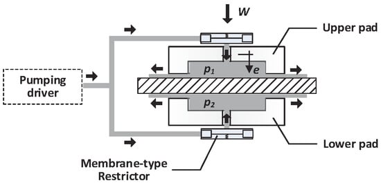
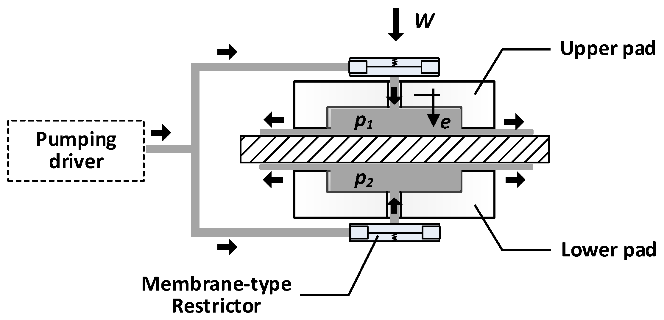
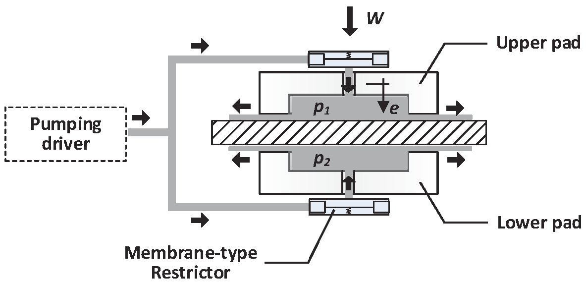
2. Bearing Models for the Opposed-Pad Configuration

In order to get a wider working range and reduce contaminants, the bearing is often designed as a closed form structure. The closed form structure often contains a certain number of opposed pads, which have ability to withstand the forces in two opposing directions. An opposed-pad bearing is illustrated in Figure 1, and the electrical network analogy of the opposed-pad bearing is illustrated in Figure 2.

For a single-pad bearing two dimensionless parameters can be adopted for designing a membrane restrictor [14]. The first one is the dimensionless stiffness of the membrane $K_r^{*}$, and the other one is the design restriction ratio $\lambda$. However concerning the similarity of working principles, these parameters will also be adopted for designing the membrane restrictors deployed in the opposed-pad bearing. The load capacity of an opposed-pad bearing was derived from the combination of the load of the upper pad and the load of the lower pad such as:

$$\begin{array}{cc}W\hfill & =W_1-W_2=p_1{A}_{e1}-p_2{A}_{e2}\hfill \\ & =P_s{A}_{e1}\left({\overline{p}}_1-\frac{1}{\alpha }{\overline{p}}_2\right)\hfill \end{array}$$

(1)

where ${\overline{p}}_1$(=$p_1/p_s)$ and ${\overline{p}}_2$(=$p_2/p_s)$ are the pressure ratios of the upper recess and the pressure ratio of the lower recess, respectively, and $\alpha$ is the ratio of the effective area of the upper pad to the effective area of the lower pad (=$A_{e1}/A_{e2}$). The pressure ratios of the pads, ${\overline{p}}_1$ and ${\overline{p}}_2$, can be calculated from an equivalent equation derived from a force equivalent of the membrane.

For a membrane restrictor, with reference to Figure 3, because the net force from the pressures applied on the membrane is equal to the spring force induced from a membrane deformation, the following equation should be satisfied:

$$\xi =\frac{x}{{\ell }_0}=\frac{1-\overline{p}}{K_r^{*}}$$

(2)

where the membrane deformation ratio $\xi$ is the ratio of membrane deformation x and assembling clearance of the membrane ${\ell }_0$. The term $K_r^{*}$ is known as the dimensionless stiffness of the membrane:

$$K_r^{*}=K_r\frac{{\ell }_0}{p_s{A}_r}$$

(3)

where $K_r$ is the stiffness of the membrane (assumed to be a constant), ${\ell }_0$ is the designed clearance for assembling the membrane of the restrictor (the clearance of the restriction plane when no force is exerted on the membrane), $p_s$ is supply pressure, and $A_r$ is the effective area of the restricting plane. For a circular restricting plane, when outer radius $r_2$ and radius ratio $\gamma$ are known, the effective area $A_r$ can be calculated as [1]:

$$A_r=\frac{1}{2}\pi r_2^2\frac{1-{\left(\gamma \right)}^2}{ln(1/\gamma )}$$

(4)

The lubricant flow rate through the bearing pad is equivalent to that at the membrane restrictor. Therefore the pressure ratio of the pad is given by:

$$\overline{p}=\frac{(1-\overline{p})R}{R_r}=\frac{(1-\overline{p})}{\lambda }\frac{R_{ri}}{R_r}\frac{R}{R_0}$$

(5)

The design restriction ratio $\lambda$ is one of the dimensionless design parameters, defined as:

$$\lambda =\frac{R_{ri}}{R_0}$$

(6)

where $R_{ri}$ is the flow resistance of the restrictor when the deformation of membrane is zero (i.e., no force is exerted on the membrane) [1]:

$$R_{ri}=\frac{\eta }{{\ell }_0^3}\frac{6}{\pi }log\frac{1}{\gamma }$$

(7)

Additionally, R is the flow resistance of the bearing pad. The flow resistance is related to the geometry and to the dimension of the pad and the recess, and it is inversely proportional to the third power of the bearing clearance h. $R_0$ is the flow resistance of the bearing pad when the bearing clearance h is at a designed value $h_0$.

According to the resistance law of third power, the resistance ratio of the membrane restrictor is given by [1]:

$$\frac{R_{ri}}{R_r}={(1-\xi )}^3$$

(8)

Making use of Equations (2), (5) and (8), the pressure ratio can be expressed as:

$$\overline{p}=\frac{1}{\lambda \frac{R_0}{R}\frac{{K_r^{*}}^3}{{(k_r^{*}-1+\overline{p})}^3}+1}$$

(9)

When the dimensionless stiffness $K_r^{*}$ and the design restriction ratio $\lambda$ are given, the relation between the pressure ratio $\overline{p}$ and the resistance ratio $R_0/R$ can be solved numerically. For the upper pad of the bearing, the resistance ratio of the bearing surface can be written as a function of a bearing eccentricity $ϵ$:

$$\frac{R_0}{R_1}=\frac{h_1^3}{h_0^3}={(1-ϵ)}^3$$

(10)

Therefore, Equation (9) can be rewritten as:

$${\overline{p}}_1=\frac{1}{\lambda {(1-ϵ)}^3\frac{{K_{r1}^{*}}^3}{{(K_{r1}^{*}-1+{\overline{p}}_1)}^3}+1}$$

(11)

For the lower pad of the bearing, the resistance ratio is:

$$\frac{R_0}{R_2}=\frac{h_2^3}{h_0^3}={(1+ϵ)}^3$$

(12)

and the equation of the pressure ratio is:

$${\overline{p}}_2=\frac{1}{\lambda {(1+ϵ)}^3\frac{{K_{r2}^{*}}^3}{{(K_{r2}^{*}-1+{\overline{p}}_2)}^3}+1}$$

(13)

When ${\overline{p}}_1$, ${\overline{p}}_2$ are known, using Equations (11) and (13), respectively, the load capacity of the opposed-pad bearing can be calculated by Equation (1). Consequently, the stiffness of the bearing can be estimated as:

$$K=\frac{dW}{de}=\frac{p_s{A}_{e1}}{h_0}\frac{d}{dϵ}\left({\overline{p}}_1-\frac{1}{\alpha }{\overline{p}}_2\right)$$

(14)

Similar to the single-pad case, the stiffness of the opposed-pad bearing is inversely proportional to the reference clearance of the bearing. A thinner reference clearance leads to a higher bearing stiffness and a lower power consumption, however a high demand of manufacturing accuracy follows.

In the following section, the effects of the design parameters of membrane restrictors on an opposed-pad bearing are presented. The calculated results will indicate that when the two dimensionless design parameters are properly given, the opposed-pad bearing should comparably offer great static stiffness over a wide load range.

3. The Effects of Restrictor Design on Bearing Performance

The bearing models described in Section 2 were implemented in a Matlab program. The parameters and levels studied are shown in

Table 1. Bearing parameters and levels used for the analysis

Parameters	Levels
Effective area ratio ($\alpha$)	1.0, 2.0
Dimensionless stiffness of upper membrane ($K_{r1}^{*}$)	1.33, 1.50, 2.00
Dimensionless stiffness of lower membrane ($K_{r2}^{*}$)	1.33, 1.50, 2.00
Design restriction ratio ($\lambda$)	0.1, 0.25, 0.5

. The upper pad and lower pad are equally sat with three levels of the design restriction ratio—$\lambda$ = 0.1, 0.25, and 0.5—for the calculation. When the bearing eccentricity is varied, the corresponding pressure ratios, ${\overline{p}}_1$ and ${\overline{p}}_2$, can be estimated by Equations (11) and (13), respectively. The carried load W is then estimated using Equation (1), given the pressure ratios ${\overline{p}}_1$ and ${\overline{p}}_2$.

Figure 4, Figure 5 and Figure 6 show the effects of the dimensionless membrane stiffness on the clearance ratio, $h/h_0$, as a function of the dimensionless loading $W/A_{e1}{p}_s$, where in the figures $K_{r1}^{*}$ = 1.33, 1.50, and 2.00, respectively. The results calculated with the effective area ratio $\alpha =2.0$ (unequal opposed-pad bearings) are depicted with green lines. Figure 7 shows the fundamental difference of the working range of the opposed-pad configuration compared to the single-pad bearing. For all cases depicted in Figure 7, the membrane restrictor has a dimensionless stiffness, $K_r^{*}$, of 1.33 and a design restriction ratio, $\lambda$, of 0.25. Figure 8 shows the chances of further improving the bearing performance by providing different design parameters for each pad. Three different parameter combinations were calculated with a design restriction ratio, $\lambda$, of 0.25 and an effective area ratio, $\alpha$, of 1.0. Examining these results, the following observations can be made:

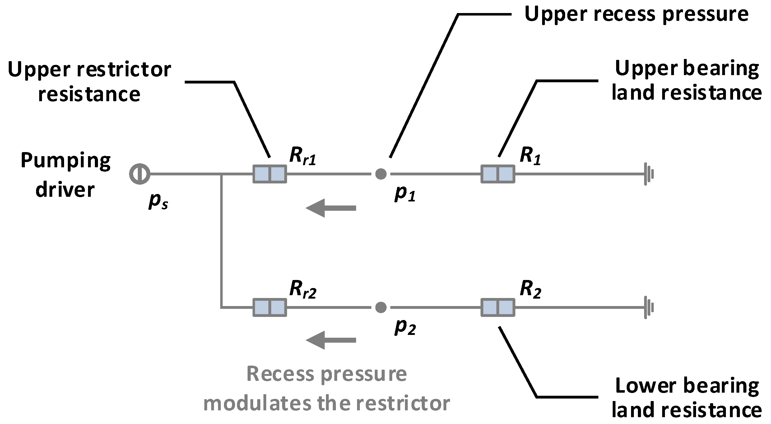
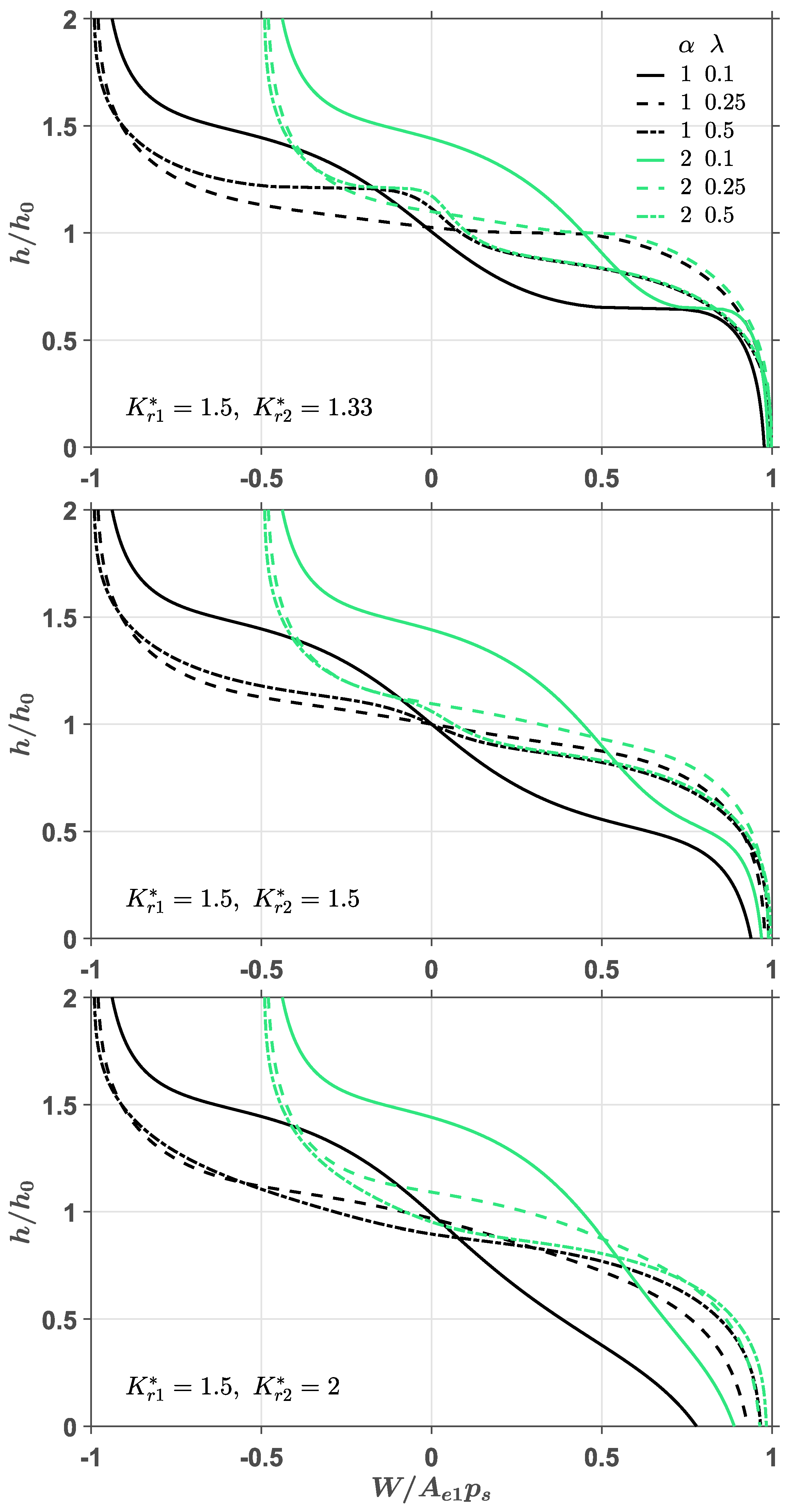
• A consistent, relatively good performance can be observed for a dimensionless membrane stiffness, $K_r^{*}$, of 1.33 and a design restriction ratio, $\lambda$, of 0.25. In this case, the bearing clearance is maintained at an almost constant level over a wide range of the dimensionless loading. In addition, the system performance for the opposed-pad bearing is less sensitive to the change of membrane stiffness, compared with that for the single-pad case presented in Reference [14].
• Within a small eccentricity range, i.e., $h/h_0\approx 1$, the benefit of choosing the design restriction ratio $\lambda =0.25$ is also significant. For the case of zero eccentricity, a good bearing stiffness can generally be obtained even if the dimensionless stiffness of the membrane $K_r^{*}$ is not the optimal value of 1.33.
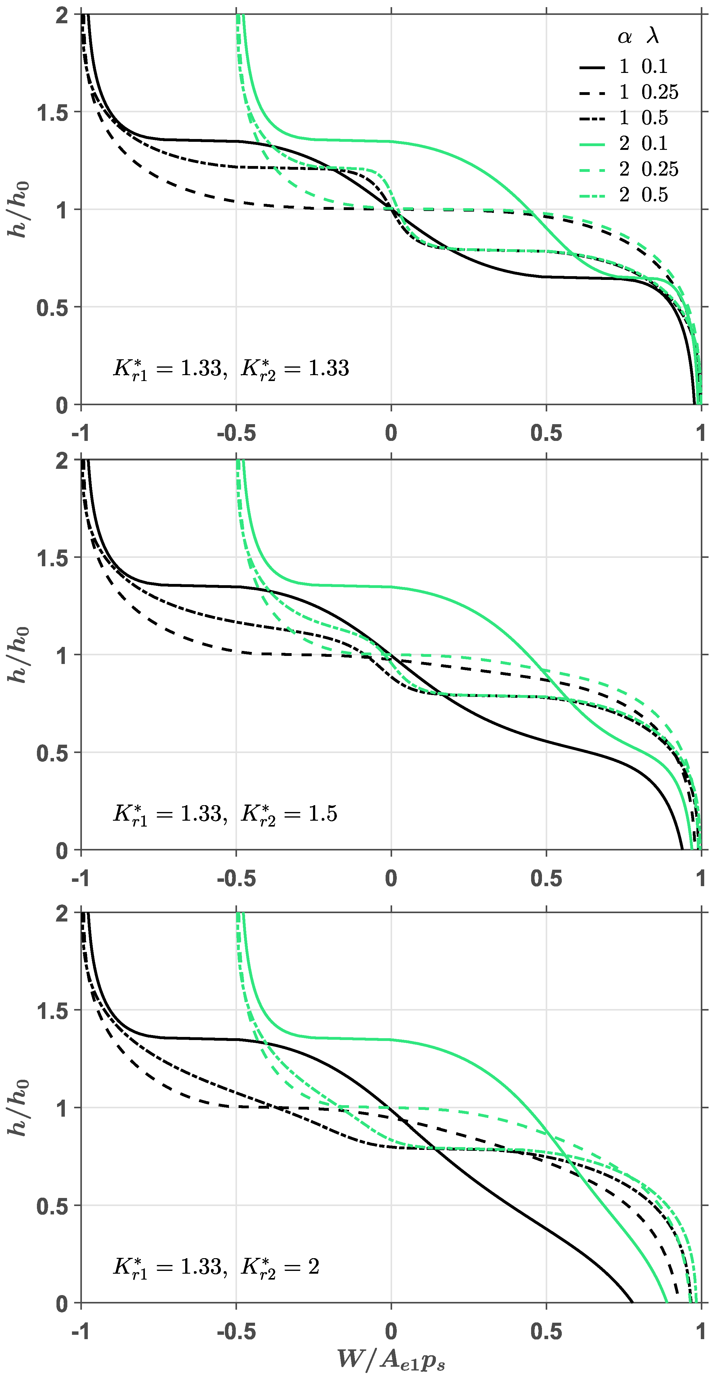
• As shown in Figure 4, it is interesting to find that the displacement of the bearing is dominated by the value of $K_{r2}^{*}$ when the dimensionless loading is positive and $\lambda$ is small (e.g., $\lambda =0.1$). This phenomenon is also revealed in Figure 5 and Figure 6. After carefully examining the variation of pressure in both pads, it is found that when the dimensionless loading is positive, the pressure in the upper pad, for all loading cases, is maintained at a high level, while the pressure in the lower pad is significantly changed as the loading is changed. This is because when a smaller design restriction ratio $\lambda$ is adopted, the flow resistance of restrictor $R_{r1}$ is smaller and hence a higher recess pressure p will appear, even when no load was applied ($W/A_{e1}{p}_s=0$). The increase in loading will result in a decrease in bearing clearance ratio ($h/h_0$) and hence a lower resistance of the lower pad. However, the increase in upper pad pressure is limited since the upper pad pressure is already quite high when no load is applied. Therefore, the lower pad dominates the performance of the bearing. Similar phenomenon can be observed when the dimensionless loading is negative.
• From Figure 4, Figure 5 and Figure 6, for the case $K_{r2}^{*}=1.33$, it is found that when the dimensionless load is positive, the effects of $K_{r1}^{*}$ on the clearance ratio of the bearing increases as a larger $\lambda$ is adopted (e.g., $\lambda =0.5$). When $\lambda =0.25$, the value of $K_{r2}^{*}$ still dominates the performance of the system within the positive load range. However, the effects of $K_{r1}^{*}$ appear. This is because when a larger design restriction ratio $\lambda$ is adopted, the flow resistance of restrictor $R_{r1}$ is larger, and hence a lower pressure on the upper pad $p_1$ will be present when no load is applied ($W/A_{e1}{p}_s=0$). Increasing the loading will decrease the clearance ratio and, hence, leads to a higher resistance of the upper pad. Therefore, the increase in the upper pad pressure is larger since the upper pad pressure is lower than the previous case when no load is applied.
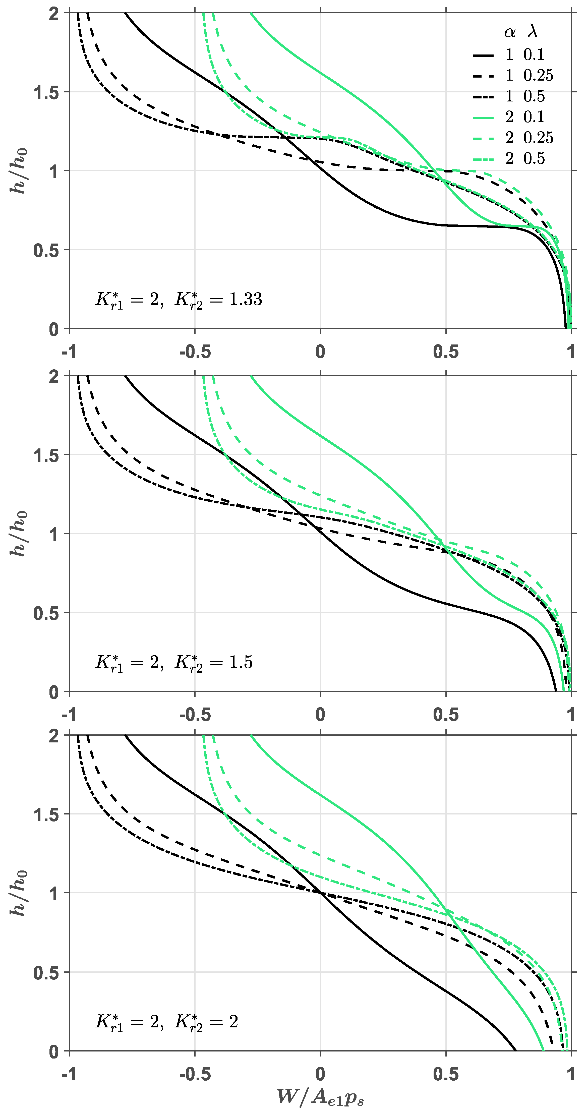
• A further increase in the design restriction ratio generally increases the dominance of $K_{r1}^{*}$ in the positive load range. It becomes difficult to identify the optimal parameter combinations such that the system can have the best performance. The dimensionless membrane stiffness $K_r^{*}$ of 1.33 for both pads is no longer the optimal solution, when the applied load is small. A small load change makes a big clearance change; it is indicated that the bearing stiffness is quite low at this loading range. Instead, the dimensionless membrane stiffness $K_r^{*}$ of 2.00 for both pads can provide a more consistent bearing stiffness over a wide load range.
• Comparing the results with the effective area ratio $\alpha =2.0$ (depicted as green lines), it is shown that similar trends and conclusions can be derived for both cases. The major difference is the loading range for negative loading is roughly half of that for positive loading. This is so because the effective area of the lower pad is only half of the effective area of the upper pad.
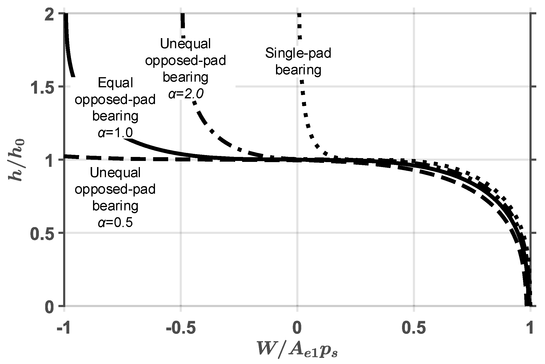
• As shown in Figure 7, the opposed-pad bearing can withstand two principal forces coming from two opposite directions, and the bearing will have great stiffness even when the bearing load approaches zero. However the single-pad bearing can withstand only a principal force in one direction, and the bearing stiffness will be dramatically degraded when the bearing load becomes small.
• Decreasing the effective area ratio $\alpha$, generally increases the applicable working range of the bearing, i.e., it makes the flat region of the curve wider, however the eccentricity at a high loading condition, $W/A_{e1}{p}_s>0.5$, is increased. For the single-pad bearing, the flat region of the curve is between $W/A_{e1}{p}_s$ = 0.2∼0.5. For the unequal opposed-pad bearing ($\alpha =2.0$), the flat region of the curve is increased to 0∼0.5. For the equal opposed-pad bearing ($\alpha =1.0$), the flat region becomes much wider, and extends to −0.4∼0.4.
• Based on the examined results shown in Figure 4, Figure 5 and Figure 6, when the design parameters for both pads are given by $K_{r1}^{*}=K_{r2}^{*}=1.33$ and $\lambda =0.25$, the bearing performance is generally good. However, for some special loading demands, e.g., the bearing is designed to withstand high loads, different design parameters for each pad may help to fulfill the requirements. The chance for further improvements of the bearing performance for high loading demands is shown in Figure 8. From this figure, when the bearing load is high, it is observed that when different design parameters for each pad are given, higher bearing stiffness can be obtained. The calculation results show that the parameter combination of $K_{r1}^{*}=4.00$ and $K_{r2}^{*}=1.33$ has better bearing stiffness within the load range $W/A_{e1}{p}_s=$0.3∼0.6.

4. Design Procedure

A procedure for designing the membrane restrictor for an opposed-pad bearing to achieve high static stiffness is introduced in this section. The procedure is centered on two design criteria: maximizing the bearing stiffness when the eccentricity of the bearing is zero, and maximizing the applicable load range when the eccentricity of the bearing does not exceed $\pm 0.6$. A very low rotating speed of the bearing is assumed such that pressures produced by inertial effects can be ignored.

The typical form of a membrane restrictor providing high static bearing stiffness, as shown in Figure 3, consists of four basic design elements: the inner radius of the restricting plane $r_1$, the outer radius of the restricting plane $r_2$, the assembling clearance ${\ell }_0$, and the membrane stiffness $K_r$. The combination of these design elements with supply pressure $p_s$ and reference flow resistance $R_0$ constitutes the two dimensionless design parameters, $K_r^{*}$ and $\lambda$. As aforementioned, the operating characteristics of the membrane restrictor can generally be determined by these two design parameters. The information needed for use in the design procedure is depicted in Figure 9, Figure 10 and Figure 11, which are fetched from the results calculated with the parameter combination, $K_{r1}^{*}=K_{r2}^{*}=1.33$ and $\lambda =0.25$.

Figure 9 illustrates the normal operating region of the opposed-pad bearings compensated with membrane restrictors when the effective area ratio $\alpha$ is varied. The maximum load is calculated on the assumption that a designed operating eccentricity beyond the range $\pm 0.6$ is undesirable in order to avoid the overload collapse of the bearings.

Figure 10 illustrates the relationship between the maximum load ratio $W_{pos}/W_{neg}$ and the effective area ratio $\alpha$. The information depicted in Figure 10 is determined from Figure 9, and is convenient for use in the design procedure. When the maximum rated loads, $W_{pos}$ and $W_{neg}$, are given, an appropriate area ratio $\alpha$ for the opposed-pad bearing can be readily determined.

Figure 11 illustrates the stiffness of the bearings at the positive maximum load condition and the negative maximum load condition. The stiffness values are calculated by Equation (10) with the parameter combination, $K_{r1}^{*}=K_{r2}^{*}=1.33$ and $\lambda =0.25$. When $\alpha >1$, the minimal bearing stiffness appears with the negative maximum load condition. With an area ratio $\alpha$, the information of the minimal stiffness of the bearing in the operating eccentricity range $-0.6<ϵ<0.6$ can be found, as shown in Figure 11.

The instructions included in the procedure described below can help to design an opposed-pad bearing compensated with membrane restrictors, with the goal of achieving a high static stiffness:

• Give the maximum positive load ($W_{pos}$)
• Give the maximum negative load ($W_{neg}$)
• Determine the area ratio ($\alpha$)
  Having given a maximum positive load $W_{pos}$ and a maximum negative load $W_{neg}$, read an appropriate area ratio $\alpha$ from Figure 10.
• Decide on a supply pressure ($p_s$)
  For given a high supply pressure: a high bearing capacity, a high minimal bearing stiffness, and a small required bearing area will be obtained. However, a high pumping power follows.
• Determine the effective areas ($A_{e1}$ and $A_{e2}$)
  When the maximum load $W_{pos}$ (or $W_{neg}$), the supply pressure $p_s$, and the area ratio $\alpha$ are known, the effective areas of the bearing can be determined from Figure 9.
• Decide on a reference clearance ($h_0$)
  When the bearing speed is very low, there is no evidence that the bearing performance can benefit by a large value of the reference clearance. Large pad clearance means high lubricant flow rate, therefore the pumping power is likely to be high. For the purpose of decreasing the power consumption, a small clearance is suggested. The small clearance should be consistent with capabilities and economics of manufacturing.
• Determine the minimal bearing stiffness ($K_m$)
  With the area ratio $\alpha$, the minimal stiffness of the bearing under the designed operating work range can be determined from Figure 11.
• Check the minimal bearing stiffness ($K_m$)
  If the minimal stiffness is not greater than the specified value, consider decreasing the reference clearance $h_0$ in step 6; the bearing stiffness is generally inversely proportional to the bearing clearance. Some issues, however, will follow when the reference clearance is set too small. Smaller clearance will require better surface finish, which necessitates longer manufacturing time and higher production cost. Even when the bearing works at a low rotating speed, making the clearance extremely small also leads to high viscous friction and high lubricant temperature. Gradually decreasing the reference clearance $h_0$ is therefore, not always a feasible option. Instead, one can consider increasing the supply pressure in step 4 to improve the minimal stiffness.
• Determine the dimensionless effective area ($A_e^{*}$)
  The dimensionless effective area (a.k.a. bearing area, or area shape factor) is a loading-capacity factor related to the geometry of the bearing pad, such as its length-to-width ratio, fillet, and recess dimension, etc. Depending on applications, many different geometries have been introduced, and detailed calculations of $A_e^{*}$ can be found in many early reports [1,2,3]. For designing convenience, a dimensionless effective area will be given for both pads.
• Determine the minimal required projected areas ($A_{1,min}$ and $A_{2,min}$)
  When the effective areas $A_{e1}$ and $A_{e2}$, and the dimensionless effective area $A_e^{*}$ are known, the minimal required projected areas can be determined. The term minimum indicates that a smaller size of the area should not be given.
• Determine the actual bearing areas ($A_1$ and $A_2$)
  The actual bearing area for the upper pad should be chosen as $A_1>A_{1,min}$ and conform to the size limits in engineering practices. Then the actual bearing area for the lower pad $A_2$ can be calculated with the area ratio $\alpha$ such that $A_2=A_1/\alpha$. Generally, larger bearing area leads to better bearing load capacity, however, a higher power loss coming from the viscous friction will follow.
• Determine the bearing dimensions
• Determine the dimensionless flow resistance ($R^{*}$)
  Similar to the dimensionless effective area $A_e^{*}$, the dimensionless flow resistance $R^{*}$ ($=R_0{h}_0^3/\eta$) is a flow factor related to the geometry of the bearing pad. The dimensionless flow resistance can be calculated by the reported models from References [1,3]. Sometimes it will be presented in a inversely proportional form ($1/R^{*}$); in terms of the flow shape factor [2].
• Decide on a radius ratio of the restricting plane ($\gamma$)
• Determine the assembling clearance of membrane (${\ell }_0$)
  Making use of Equations (6) and (7), the assembling clearance of the membrane can be determined as:

  $${\ell }_0=h_0\sqrt[3]{\frac{1}{\pi }\frac{6}{\lambda R^{*}}ln(1/\gamma )}$$

  (15)

  For maximizing the bearing stiffness at zero eccentricity, it is suggested to give $\lambda =0.25$.
• Determine the minimal membrane stiffness ($K_{r,min}$)
  The minimal requirement for the membrane stiffness is given to ensure the dimensionless membrane stiffness $K_r^{*}$ is larger than the optimal value of 1.33. The reason for this is to avoid an operating instability without compromising the bearing load capacity. Theoretically, a negative bearing stiffness appears when the dimensionless membrane stiffness $K_r^{*}$ is smaller than 1.33 [14].
  When the dimensionless membrane stiffness $K_r^{*}$, the supply pressure $p_s$, the effective area of the restricting plane $A_r$, and the assembling clearance of the membrane ${\ell }_0$ are given, then the minimal membrane stiffness can be determined as:

  $$K_{r,min}=K_r^{*}\frac{p_s{A}_r}{{\ell }_0}$$

  (16)

  For maximizing the bearing stiffness at zero eccentricity, it is suggested that $K_r^{*}=1.33$.
• Decide on the inner radius of the restricting plane ($r_1$)
• Determine the outer radius of the restricting plane ($r_2=r_1/\gamma$)
• Determine the actual membrane stiffness ($K_r$)
  The effective stiffness of a circular membrane plate (diaphragm) can generally be determined by the deformation of the membrane with an applied force. The deformation can be estimated by the equations for plates and shells [15]. When a plate material is chosen, the elasticity modulus and the Poisson’s ratio of the membrane plate is determined. With this information and the dimensions of the plate, including $r_1$ and $r_2$, the membrane stiffness can be calculated. In engineering practice, making the membrane stiffness match the optimal one is trivial. In order to obtain a great bearing stiffness without compromising the bearing load capacity, a larger membrane stiffness, i.e., $K_r>K_{r,min}$, should be given.
• Revise the supply pressure ($p_s$)
  When the actual membrane stiffness is given, the actual supply pressure, needed for making the restrictor operate with good design features, should be modified to:

  $$p_s=\frac{K_r}{K_r^{*}}\frac{{\ell }_0}{A_r}$$

  (17)

For the bearing compensated with membrane restrictors, the load capacity and the static stiffness of the bearing are theoretically independent of the lubricant viscosity, when the viscosity is assumed constant everywhere and the laminar flow is assumed. In order to decrease the power consumption for a low operating speed, a higher viscosity is preferred.

The dimensionless effective area $A_e^{*}$ and dimensionless flow resistance $R^{*}$, as mentioned in instructions 9 and 13, respectively, are both geometry-related parameters. Having chosen a bearing geometry, both parameters are determined. In practice, the bearing geometry can be chosen by a minimizing power criterion for four reasons:

• Making the temperature rise of the lubricant small.
• Making the viscosity variations small. (Large viscosity variations will make pressure control difficult.)
• Making the thermal distortions of the bearing structure small.
• Making the time for temperature stabilization of the bearing structure short.

High power consumption leads to high temperature rise and a low viscosity of the lubricant. This may cause the bearing and the restrictor to vary from operating in the laminar regime to the turbulent regime, and therefore affect the bearing’s performance. The power consumption can generally be improved by choosing a proper pad geometry in the different speed regimes. At zero or very low speeds, pumping power is only needed to be taken into consideration. When the bearing speed is increased, the effect of viscous friction is larger, therefore the friction power increases. A pad with a small land and a large recess is preferred for a high speed bearing. Detailed discussions on temperature and power consumption issues are described by Bassani and Piccigalo [1].

In order to evaluate the effect of the viscous friction, the dimensionless effective friction area $A_f^{*}$, should be involved. When the dimensionless flow resistance $R^{*}$ and the dimensionless effective friction area $A_f^{*}$ are given, the optimal viscosity for minimizing the total power consumption (including pumping power and friction power) in the different speeds regime can generally be calculated [13].

5. Conclusions

The effects of different design parameter combinations for membrane restrictors are studied in this article. The main conclusion drawn from this work is that compared to the single-pad system—where the performance of the system is dominated by two dimensionless design parameters, the dimensionless stiffness of the membrane $K_r^{*}$ and the design restriction ratio $\lambda$—the opposed-pad bearing has a much wider applicable working range.

It was also found that, for the opposed-pad bearing, the design restriction ratio $\lambda$ is an even more important design parameter than the dimensionless stiffness of the membrane $K_r^{*}$. The results show that when the bearing eccentricity is small, a $\lambda$ of 0.25 still results in high stiffness over a wide load range, even when $K_r^{*}$ is not the optimal value of 1.33.

Additionally, the chance for further improvement of the bearing performance is also revealed in this article. For high loading demands, the bearing stiffness can benefit from providing different design parameters for each pad of the bearing.

A design procedure with three informative illustrations is given. The steps and key parameters described in the procedure are standardized on the examined results in this article. The procedure aims at obtaining a high static stiffness of the opposed-pad bearing.

References

1. Bassani, R.; Piccigallo, B. Hydrostatic Lubrication; Elsevier: Amsterdam, The Netherlands, 1992. [Google Scholar]
2. Rowe, W.B. Hydrostatic, Aerostatic and Hybrid Bearing Design; Butterworth-Heinemann: Amsterdam, The Netherlands, 2012. [Google Scholar]
3. Hamrock, B.J.; Schmid, S.R.; Jacobson, B.O. Fundamentals of Fluid Film Lubrication; Marcel Dekker: New York, NY, USA, 2004. [Google Scholar]
4. Mohsin, M.E. The use of controlled restrictors for compensating hydrostatic bearings. In Advances in Machine Tool Design and Research, Proceedings of the 3rd International MDTR Conference, Birmingham, UK, September 1962; Pergamon Press: New York, NY, USA, 1962; pp. 429–442. [Google Scholar]
5. DeGast, J.G.C. A new type of controlled restrictor (M.D.R.) for double film hydrostatic bearings and its application to high-precision machine tools. In Advances in Machine Tool Design and Research, Proceedings of the 7th International MDTR Conference, Birmingham, UK, September 1966; Pergamon Press: New York, NY, USA, 1966; pp. 273–298. [Google Scholar]
6. Mohsin, M.E.; Morsi, S.A. The dynamic stiffness of controlled hydrostatic bearings. J. Lubr. Technol. 1969, 91, 597–608. [Google Scholar] [CrossRef]
7. Rowe, W.B.; O’Donoghue, J.P. Diaphragm valves for controlling opposed pad bearings. Proc. Inst. Mech. Eng. 1969, 184, 1–9. [Google Scholar]
8. Cusano, C. Characteristics of externally pressurized journal bearings with membrance-type variable-flow restrictors as compensating elements. Proc. Inst. Mech. Eng. 1974, 188, 527–536. [Google Scholar]
9. Phalle, V.M.; Sharma, S.C.; Jain, S.C. Influence of wear on the performance of a 2-lobe multirecess hybrid journal bearing system compensated with membrane restrictor. Tribol. Int. 2011, 44, 380–395. [Google Scholar] [CrossRef]
10. Liu, Z.; Pan, W.; Lu, C.; Zhang, Y. Numerical analysis on the static performance of a new piezoelectric membrane restrictor. Ind. Lubr. Tribol. 2016, 68, 521–529. [Google Scholar] [CrossRef]
11. O’Donoghue, J.P.; Rowe, W.B. Hydrostatic bearing design. Tribology 1969, 2, 25–71. [Google Scholar] [CrossRef]
12. O’Donoghue, J.P.; Rowe, W.B. Hydrostatic bearing design: Supplement for unequal opposed pads. Tribology 1969, 2, 225–232. [Google Scholar] [CrossRef]
13. Rowe, W.B.; O’Donoghue, J.P.; Cameron, A. Optimization of externally pressurized bearings for minimum power and low temperature. Tribology 1970, 3, 153–157. [Google Scholar] [CrossRef]
14. Lai, T.H.; Chang, T.Y.; Yang, Y.L.; Lin, S.C. Parameters design of a membrane-type restrictor with single-pad hydrostatic bearing to achieve high static stiffness. Tribol. Int. 2017, 107, 206–212. [Google Scholar] [CrossRef]
15. Timoshenko, S.; Woinowsky Krieger, S. Theory of Plates and Shells; McGraw-Hill: New York, NY, USA, 1959. [Google Scholar]
Figure 1. A sketch of a hydrostatic opposed-pad bearing. Where W is bearing load, p 1 and p 2 are the recess pressure of the upper pad and the lower pad respectively, and e is the eccentricity of the bearing.
Lubricants 06 00071 g001
Figure 2. A sketch of the electrical circuit analog of a hydrostatic opposed-pad bearing. Where R r 1 and R r 2 are the flow resistance of the upper restrictor and the lower restrictor respectively, R 1 and R 2 are the flow resistance of the upper pad and the lower pad respectively, and p s is supply pressure.
Lubricants 06 00071 g002
Figure 3. A sketch of a single-pad bearing with a membrane restrictor. Where r 1 is the inner radius of the restricting plane, r 2 is the outer radius of the restricting plane, and 0 is the assembling clearance of membrane.
Lubricants 06 00071 g003
Figure 4. Effects of the dimensionless stiffness of both pads on the clearance ratio of bearing. Where α is effective area ratio, λ is design restriction ratio, h / h 0 is the clearance ratio of bearing, A e 1 is the effective area of the upper pad, and K r 2 * is the dimensionless stiffness of the lower pad. The dimensionless stiffness of upper pad, K r 1 * , is 1.33.
Lubricants 06 00071 g004
Figure 5. Effects of the the dimensionless stiffness of both pads on the clearance ratio of the bearing, where K r 1 * = 1.50 .
Lubricants 06 00071 g005
Figure 6. Effects of dimensionless stiffness of both pads on the clearance ratio of the bearing, where K r 1 * = 2.00 .
Lubricants 06 00071 g006
Figure 7. Effects of the dimensionless loading on the clearance ratio for four bearing configurations, with K r 1 * = K r 2 * = 1.33 and λ = 0.25 .
Lubricants 06 00071 g007
Figure 8. Effects of the dimensionless loading on the clearance ratio for three design parameter combinations, with λ = 0.25 and α = 1.0 .
Lubricants 06 00071 g008
Figure 9. Normal operating region for opposed-pad bearings. Where A e 1 / A e 2 is effective area ratio (= α ).
Lubricants 06 00071 g009
Figure 10. Relationship between the maximum load ratio and the effective area ratio. Where W p o s is positive maximum load, and W n e g is negative maximum load.
Lubricants 06 00071 g010
Figure 11. The stiffness of the bearings at maximum load conditions. Where k is bearing stiffness.
Lubricants 06 00071 g011