Abstract
Solid particle erosion affects many areas, such as dust or volcanic ash in areo-engines. The development of protective materials and surface engineering is costly and time consuming. A lot of effort has been placed into the advancement of models to speed up this process. Finite element or discrete element-based models are quite successful in predicting single or multiple impacts. However, they reach their limit if an entire erosion experiment is to be simulated. Therefore, in the present work, an approach is presented which combines various aspects of the former models with probability considerations. It is used to simulate the impact of more than one billion Alumina particles onto a steel substrate. This approach permits the simulation of an entire erosion experiment on an average PC (i5-2520M CPU@2.5 GHz processor, 4 GB main memory) within about six hours. The respective predictions of wear scar and impact-mass/mass-loss curve are compared to the real experiment.
1. Introduction
Across different industries and respective locations in plants, the type and cause of solid particle erosion varies. Such particles could be volcanic ash, e.g., in aero-engines or fly ash in boilers, mineral matter in oil excavation, or exfoliated scale in steam turbines. The durability of materials can be improved in all cases through better coatings and surface engineering. A lot of effort has been placed into the development of models predicting the behavior of the latter, in order to speed up the respective development. Two major types of these models are based on finite element methods (FEM) and discrete element methods (DEM). Griffin et al. describe a three-dimensional finite element model which they used to simulate the impact of a solid, spherical shaped particle on an Alumina scale/MA956 substrate [1]. For convenience and shorter calculation time, it is commonly concentrated on a two-dimensional simulation of a single impact (e.g., [2]) or at best multiple impact (e.g., [3]) of spherical particles. Smoothed particle hydrodynamics was used to simulate the impact of angular particles on ductile material such as aluminum or aluminum alloys. Takaffoli and Papini demonstrate that this simulation technique is able to properly simulate the formation of a crater, chip separation, and material pile-up for a single impact [4]. It is even possible to estimate the ratio of incident particles that rebound or fracture on impact with good agreement using similar methods [5].
While FEM is the tool of choice to most accurately simulate a single particle’s impact, this is not the intention of the present work. In the case of finite element-based methods, the simulation of a single impact using a mesh with about 100,000 nodes would take about 15 min (private communications) on an average personal computer. This calculation time is too long to simulate an entire particle erosion experiment with billions of such impacts.
Zhao et al. proposed a particle erosion model based on the shear impact energy of these particles using discrete element method simulations. [6]. This approach is based on time steps of 5 ns and the impact of up to 7.2 × 10⁶ particles was calculated. However, the calculation time needed and the type of computer used were not specified.
Ciampini and Papini describe an approach based on cellular automata to simulate abrasive jet micromachining of masked substrate surfaces [7]. They can calculate the impact of 1.4 × 10⁷ impacts of solid particles on these surfaces within 15 h, using a 2.4 GHz quad-core Intel CPU and 2 GB of RAM. The approach of Ciampini and Papini is based on time-steps of the order of 3 ns. Thus, for the experiment considered here, only a couple of seconds could be simulated with this approach.
The aim of the work presented here is to predict the mass-loss and the shape of the erosion scar of an entire erosion experiment. In such an experiment, about two billion particles would impact on a substrate for about twenty minutes. For this, aspects of FEM, DEM, and Monte-Carlo simulations were combined to form an approach which can be carried out on a conventional personal computer in a reasonable amount of time.
2. Experimental Details
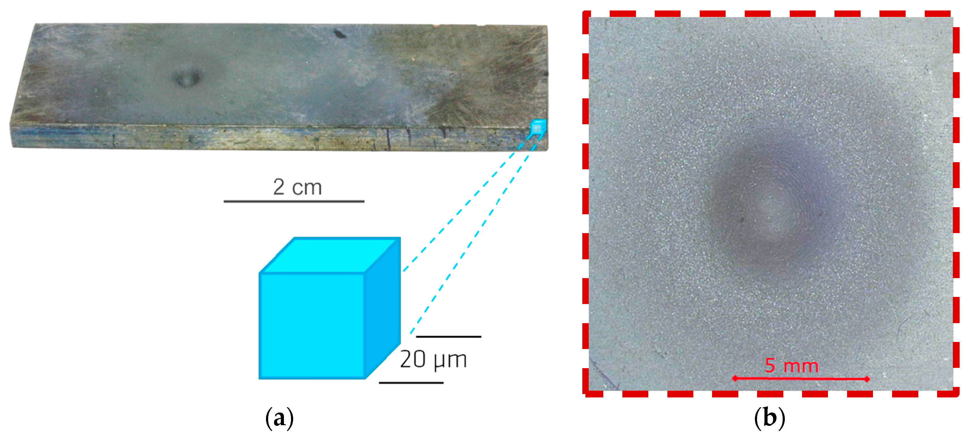
The real experiment forms the requirements for the simulation. A description of test rigs used for carrying out particle erosion experiments can be found here [8,9,10]. The erosion scar used as reference for the simulation was generated on an AISI 410 (X12Cr13) steel substrate (see Figure 1). About 100 g of Alumina particles with an average particle size of 25.4 μm (Mesh 320) were fed into a jet of hot compressed air. Thus, the particles were heated up to 600 °C and accelerated to an average velocity of 204 m/s. The substrate was hit under an impact angle of 90°.
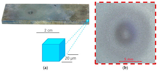
Figure 1.
(a) Erosion scar on a typical sample with a cube, indicating the build-up of the substrate via cubes; (b) top-down, enlarged view on the scar of (a).
This experiment lasted about 20 min. The material properties relevant for the calculations are summarized in Table 1. In experiments carried out by the authors, it was observed that the AISI 410 substrate showed an increase of hardness of up to 20% after a single impact of a steel or ceramic ball. It has been taken into account that the hardness of this material was increased by 20% in the contact zone upon second impact.

Table 1.
Experimentally determined properties of the erosion particles and substrate that are relevant for calculations.
The first aim of the simulation approach presented here is to generate an image comparable to the one shown in Figure 1b. Considering the size of the erosion scar, this requires the handling of an area affected by the erosion particles of 5 mm × 5 mm up to a depth of about 5 mm. If the smallest volume of interest to the simulation approach is a cube of 20 μm edge length, then more than 15 million of such cubes form the sample substrate, which have to be handled. This is the second requirement and aim of the simulation approach presented here.
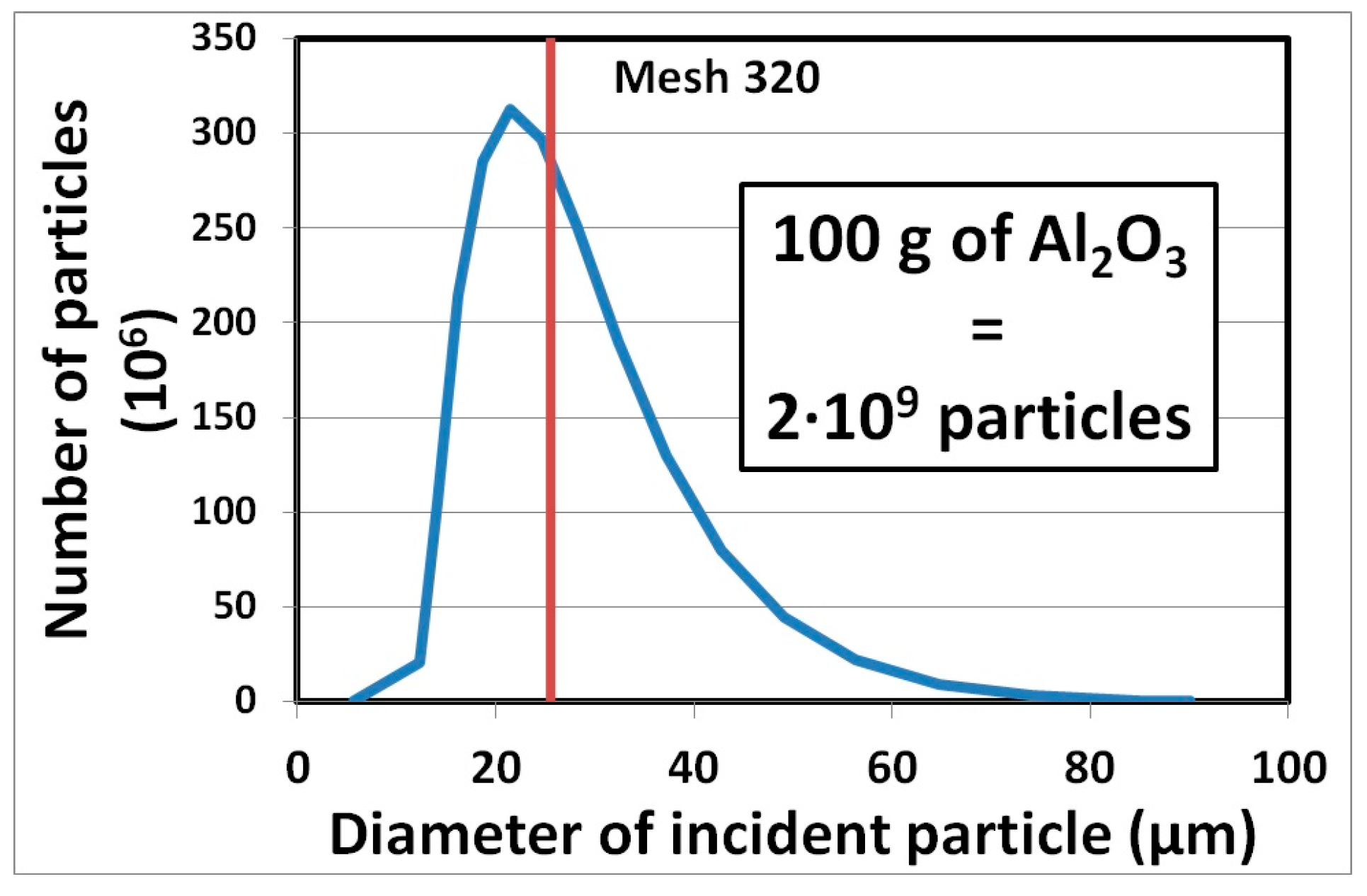
Figure 2 shows the size distribution of the Alumina powder used in the erosion test to create the scar shown in Figure 1. Although this curve exhibits a more log-normal shape, a Gaussian distribution was used as a first approximation for simplification. Adding up all particles leads to about 2 × 10⁹ impacts which have to be considered for the simulation of this erosion experiment. This is the third requirement to be fulfilled by the alternative approach presented here. The fourth one is that the respective calculations can be carried out on a standard PC (e.g., a laptop equipped with a dual core i5-2520M CPU@2.5 GHz processor and 4 GB main memory) in a reasonable amount of time (e.g., less than an eight-hour working day).

Figure 2.
Size distribution of particles used in the erosion test of Figure 1.
3. Alternative Simulation Approach
3.1. Basic Considerations
A cube (shown in Figure 1) is the smallest volume element of interest for this alternative approach to simulate erosive wear (EROW-sim). It describes a volume of same or similar properties. The shape of these elements is not important. However, cubes can be stacked without spacings in-between. Several cube elements form a row, several rows a layer and several layers form the substrate to be simulated (see Figure 3).
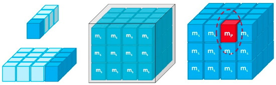
Figure 3.
Cubes are arranged in rows and layers (left) to from the substrate (middle) and interact with impacting erosion particles (right).
In this sense, EROW-sim can be considered as a discrete element-based method. However, these cubes do not move at all.
The size of the cube elements has no relevance for the approach itself in the sense that the substrate to be simulated is not limited to the sample dimensions shown in Figure 1. However, for a given size, it influences the requirement for computing time and memory. A small edge length leads to an even larger number of cubes to be handled. The plotting program used to create the wear scar simulated here is limited to 255 data rows per image. Thus, the number of cube elements per row and of rows per layer was set to 250 each. As the wear scar requires an area of 5 mm × 5 mm to be simulated, the edge length of such cubes was set to 20 μm for the simulation of this erosion experiment. The number of layers was then adjusted so that the simulation would reach the maximum main memory allocated to a single program by the operating system.
EROW-sim is a step-based method. Each particle impact is considered as a single event. The incident particle interacts with the substrate according to material properties and physical processes. The next step is carried out, i.e., the next particle impacts only occurs, if all current processes are carried out. During such processes, only relevant cubes are considered at a time. Each particle incident is treated as a local event, considering only those cubes affected by the initiated processes.
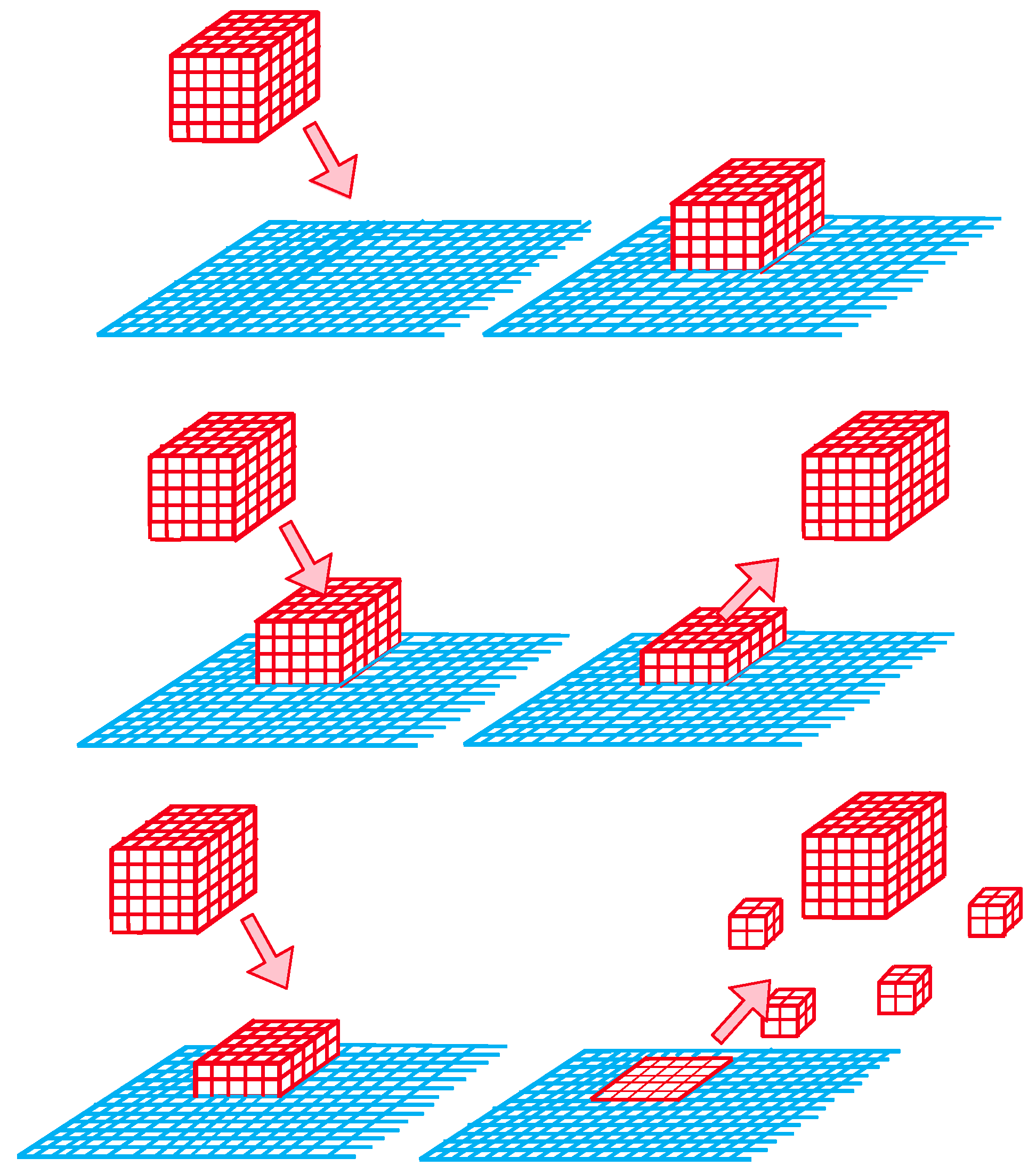
Currently, the following processes are considered (see Figure 4). If sufficient metal is present at the impact site, the incident ceramic particle has a possibility to stick (see top of Figure 4). Sticking means that the particle (or fragments of it) stays in the area of contact after the impact. This process would still be called ‘sticking’, even if the particle is covered with substrate material. In the case that such sticking particles (see center of Figure 4) are already present in the contact area, there is a chance that the pre-sticking particles will be embedded deeper into the substrate, due to the impact. Here, embedding means that a surface area is hit again by another particle, thus forcing particle material originating from an earlier impact, deeper into the substrate. The third main process considered is the possibility of the fragmentation of already embedded particles (see bottom of Figure 4) and leaving from the surface. As probabilities are considered for the different processes to take place, EROW-sim also contains certain Monte-Carlo aspects. For instance, for an incident ceramic particle to stick, there has to be sufficient metal in the contact volume. The embedding process can only take place if sticking particles are already present. The same holds true for the shattering process of a particle. The latter requires the embedding processes to have occurred before a particle can shatter/fragment. The processes described above are kept as simple as possible, as the major issue is a trade-off between accuracy of simulating a single impact or getting ~2,000,000,000 such impacts calculated in a reasonable amount of time.

Figure 4.
Main processes considered during the simulation: sticking of incident particles (top), embedding of already sticking particles (center), and shattering/fragmentation of already embedded particles (bottom).
However, these processes are strongly governed by the properties of the actual material present in the contact volume. In case metal is dominant at the impact site of the hard, ceramic particle, the penetration depth is of critical importance (confer Section 3.2). If the impact site is dominated by already sticking or embedded ceramic particles (remainders of earlier impacts), conditions for the formation of cracks in ceramics have to be considered (confer Section 3.3).
3.2. Calculation of Penetration Depth
If the impact site of the actual particle consists mainly of metal, calculating the penetration depth is essential. Forrestal et al. considered the penetration of rigid spherical-nosed rods into ductile metal targets [11]. In their work, they showed that there is no significant difference between a model for compressible or incompressible targets and experimental data in the range up to about 900 m/s. Therefore, the penetration depth p is currently calculated as follows:
where the material constant A is
and are the density of the incident particle and the substrate, respectively. L denotes the length of the incident particle in the z-direction. The radius of the particle and its spherical-shaped nose is labelled a. Here, this is basically set to the average value of the particle dimensions in x- and y-directions. The velocity of the incident particle is denoted vi, Young’s Modulus E and yield strength Y, respectively.
The calculated penetration depth in relation to the edge length of cubes is one major criterion to decide whether the currently impacting particle will stick. In the present simulation, the edge length of the cubes is set to 20 μm. Let’s assume that a penetration depth of 2 μm is calculated for a specific incident particle. A dice is rolled and in 10% (penetration depth/edge length × 100), the penetration depth would be converted to one cube and the particle would stick. In 90%, the penetration depth would be set to zero cubes, i.e., the particle bounces off the surface. In a small number of cases, there will be a large error in one direction, and in a large number of cases, a small error in the opposite direction. While the error for a specific particle might be substantial, this averages out over the billion impacts of the total experiment.
3.3. Considering Crack Formation
If an impacting particle can no longer hit the metallic substrate due to previously stuck/embedded ceramic particles, the conditions for crack formation are considered. For these considerations, the quasi-static indentation theory for erosion of brittle material is used. According to Slikkerveer et al., this theory can still be used for solid particle impact [12]. The impact velocity of some hundreds of meters per second of these particles is still much smaller than the velocity of elastic and/or plastic deformation in brittle material. Verspui et al. calculated the indentation force Fi exerted on the substrate by the impacting particle according to [13]:
where the material constant c1 is:
Here, vi is the velocity, D the diameter and the density of the impacting particle, while HS is the hardness of the substrate.
These calculations are based on the earlier work of Marshall et al. [13], dealing with the lateral crack formation in ceramics caused by a Vickers indenter. As the opening angle φ of such an indenter is 136° leading to
all such angular dependencies are neglected.
Lateral cracks are assumed to develop if a threshold load F0 is exceeded. This threshold can be calculated as [12]:
here, ES is Young’s Modulus, KIC is the fracture toughness, and HS is the hardness of the substrate.
If the threshold load F0 is exceeded by the impact force Fi of the particle, a lateral crack is formed. Its length cL can be calculated as [14]:
where the material constant c2 is:
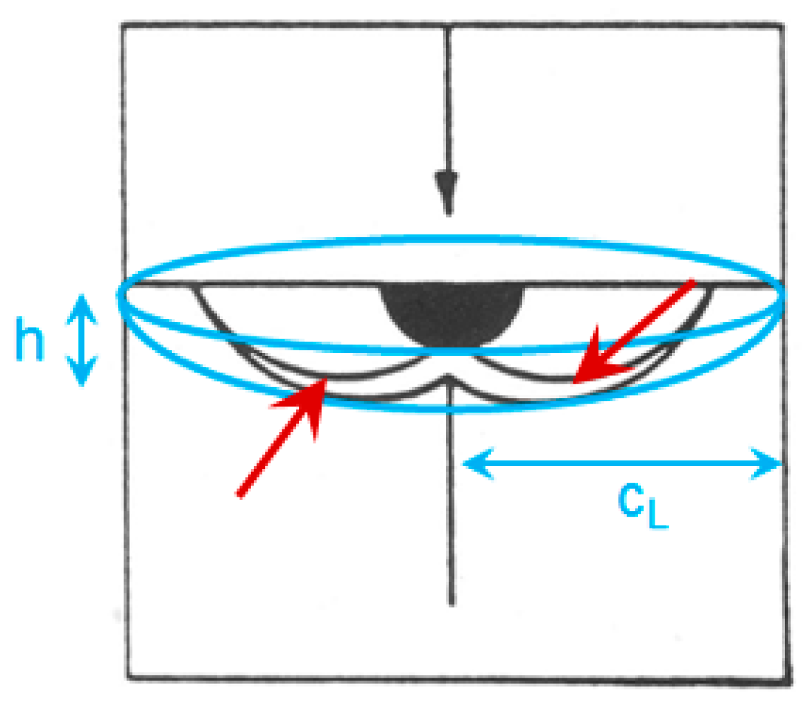
The depth h of the lateral crack is taken to be equal to the depth of the plastic zone (area marked black in Figure 5) for a Vickers indenter [14]:
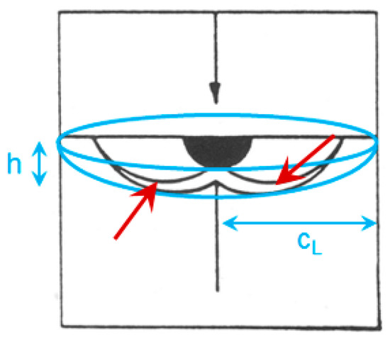
Figure 5.
On particle impact (marked by a black arrow), lateral cracks (marked with red arrows) of length cL are forming, starting at a depth h. This leads to a cap-shaped segment of mass m to be removed.
If the lateral crack starts at a depth h from the substrate surface and the lateral crack reaches the surfaces at a distance cL from its origin, a cap-shaped segment is formed (see Figure 5). The mass m of this segment is then considered to be removed per single impact on brittle material (if Fi > F0) and can be calculated as:
In case of a metal substrate, this removal of mass happens to sticking particles which are already embedded.
If the substrate is ceramic, the removal of mass according to the formation of cracks is the dominating process. Although the material used in this study is ductile metal, it is exposed to a stream of incident brittle particles. Depending on the exact impact conditions, these particles may form a protective layer at the surface (cladding). Thus, this situation would be treated as ‘brittle substrate’ and mass will be removed according to the formation of cracks. In any case, the ductile metal surface will be ‘injected’ with brittle fragments during erosion by solid particles. The substrate will no longer be as ductile as at the beginning of this process. Depending on the number of ceramic/brittle fragments of earlier impacts in the contact zone, there is a probability that mass can and will be removed according to the formation of cracks.
3.4. Creation of Impacting Particles
During the simulation, impacting particles were generated until their impacting mass reached 100 g. According to Figure 1, the average ‘diameter’ is about 26 μm. For spherical particles, this would lead to a particle volume around 8800 μm3. If particles are more angular, this ‘diameter’ would be the edge length of a cube, leading to particle volume around 16,800 μm3. Therefore, the volumes of particles were created according to a Gaussian distribution around an average volume of 12,000 μm3 and a width of ±4000 μm3 (see Figure 6a). In order to reach 100 g of impacting mass, the number of particles to be generated lies approximately between 1.6 × 10⁹ and 3.1 × 10⁹. Due to probability/Monte-Carlo issues, two simulations using exactly the same parameters will produce similar, but never the same results.
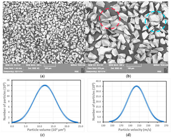
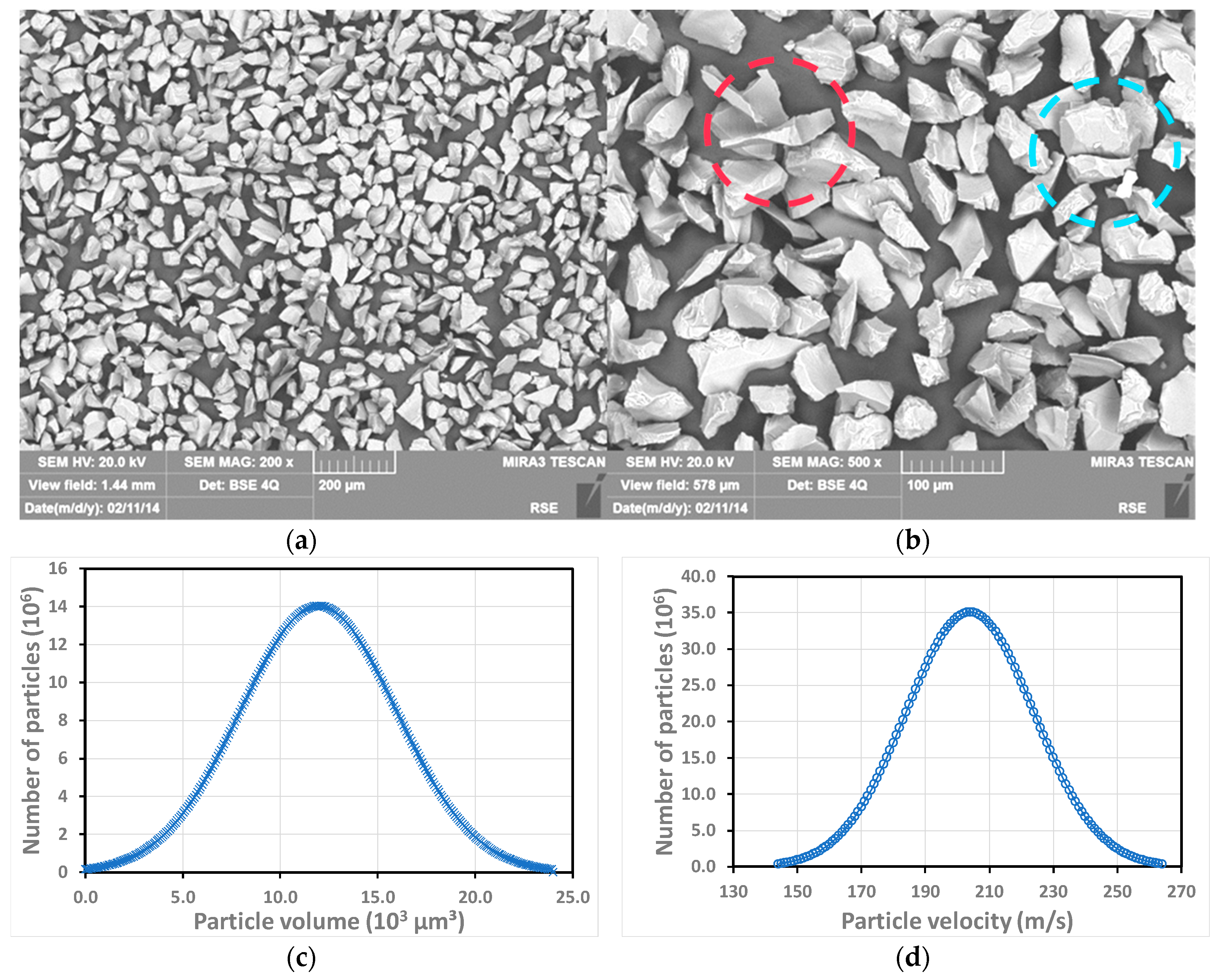
Figure 6.
(a) Volume distribution of the incident particles of the simulation; (b) SEM image of the Alumina powder used for the experiment; (c) Enlarged image of (b); (d) velocity distribution of the incident particles of the simulation.
SEM images of the erosion powder/particles are presented in Figure 6b,c. The circles highlight particles as an example for angular shape (red circle) and more spherical shape (blue circle). These images revealed that 90% of the particles were angular-shaped, causing slightly more damage (than spherical-shaped once) due to ploughing actions even under 90° impact angle. The dicing process was adjusted accordingly so that the respective number of particles for each shape was produced. If the current impacting particle had a ‘spherical’ shape, the third root was calculated of the particle volume in order to obtain the edge-length of the actual particle. If the particle is supposed to have an ‘angular’ shape, the process adopts a cuboid form, where at least one dimension is larger (which one is arbitrary) than the others. The respective calculations are carried out in micrometers. The dimensions of the particles are then converted into cubes.
Fractions of cubes are dealt with according to the procedure described for the conversion of the penetration depth. Currently, the particles are assumed always to hit with their long axis perpendicular to the surface. In order to keep calculation times low and still account for the ploughing action of angular particles, each such particle had a 5% chance to arbitrarily create excess damage.
Each particle was then ‘equipped’ with an impact velocity. The impact velocity of the particles was assumed to be Gaussian distributed around an average of 204 m/s with a width of ±20 m/s. In Figure 6b, the velocity distribution of the impacting particles is presented as it was generated during the simulation.
The characteristics of the nozzle (nozzle size, particle flow rate, standoff distance, etc.), emitting the particles in the experiment was supposed to lead to a Gaussian distribution of the particle impacts on the substrate. It was assumed that the nozzle would sit directly opposite the center of a 5 mm × 5 mm area. The width of this Gaussian distribution was assumed to be 600 μm. The impact site of each current particle was generated in a dicing process accordingly.
4. Discussion of Simulation Results, Comparison to Experiment, and Outlook
The simulation was carried out on a laptop equipped with a dual core i5-2520M CPU@2.5 GHz processor and 4 GB main memory. The smallest volumes of interest were cubes of 20 μm edge length. As the experiment was carried out at 600 °C, the material properties of particles and substrate were considered at this temperature.
The particle erosion experiment was interrupted to determine the mass loss after certain amounts of mass which had already hit the substrate. Such a mass-loss versus impact mass curve is shown in Figure 7. The blue curve marks the results obtained from the experiment. The orange curve represents the mass-loss as calculated/predicted by the simulation. During the start of the simulation, the mass-loss is negative. This is due to harder ceramic particles sticking in the softer metallic substrate.
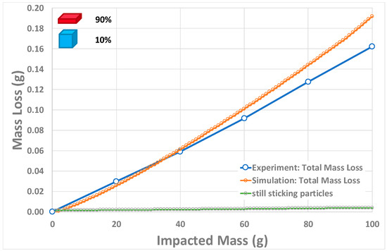
Figure 7.
Mass-loss versus impact mass curve as obtained during the experiment (blue line) and as calculated during the simulation (orange line). The green line describes the mass of the particle material still sticking in the substrate.
The impacts of about 1.75 × 10⁹ Alumina particles (100 g) on 6.25 × 10⁷ substrate cubes were simulated in about six hours. Figure 8 shows the substrate surface at the end of the simulation (top right) compared to the real sample surface (top left) at the end of the erosion test. Although the predicted image is already fairly similar to the experiment, it can be seen that in the simulation, the particles are not spreading as far. Since the same impact mass is concentrated on a smaller area, this leads to a deeper crater in the simulation (see bottom part of Figure 8). Therefore, the crater depth is overestimated by a factor of two. If a similar spreading of particles as in the experiment is chosen for the simulation, it is expected that a more precise crater depth will be obtained. However, the predicted mass-loss of 186 mg lies within 15% of the actual measured mass-loss of 162 mg of the experiment. Only the processes of Figure 4 were considered, which simplify the actual situation to keep the calculation time low. Thus, it was demonstrated that an entire erosion experiment could be simulated within a reasonable amount of time.
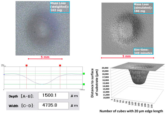
Figure 8.
Enlarged image of the wear scar of Figure 1 (top left) and image of the simulation result (top right). This figure also presents a line scan through the center of the wear scar (bottom left) and a 3D image of the crater predicted by the simulation (bottom right).
As the agreement between simulation and experiment is promising, this alternative approach will therefore be extended and pursued further. Currently, Equation (1) predicts the penetration depth of an impinging particle into the metal surface. Although it seems as if impacts under oblique angles are not accounted for, this approach provides means to simulate such impacts. It is also planned that the material properties in the contact zone will have a stronger influence on the probabilities of the processes to take place. This is especially so, if this approach is extended to different materials and coatings.
Acknowledgments
The erosion test sample was supplied by Federico Cernuschi, Ricerca sul Sistema Energetico—RSE S.p.A., Milano, Italy. This work was funded through the European Metrology Research Program (EMRP) Project IND61 Metrology to Enable High Temperature Erosion Testing (METROSION). The EMRP is jointly funded by the EMRP participating countries within EURAMET and the European Union.
Author Contributions
Mathias Woydt provided input concerning material properties and crack formation. Dirk Spaltmann set up the concepts, the simulation is based on, programmed as well as performed the simulation and wrote the paper.
Conflicts of Interest
The authors declare no conflict of interest.
References
- Griffin, D.; Daadbin, A.; Datta, S. The development of a three-dimensional finite element model for solid particle erosion on an alumina scale/MA956 substrate. Wear 2004, 256, 900–906. [Google Scholar] [CrossRef]
- Di, J.; Wanga, S.; Zhang, L.; Cai, L.; Xie, Y. Study on the erosion characteristics of boride coatings by finite element analysis. Surf. Coat. Technol. 2018, 333, 115–124. [Google Scholar] [CrossRef]
- Zheng, C.; Liu, Y.; Chen, C.; Qin, J.; Zhang, S. Finite element analysis on the dynamic erosion process using multiple-particle impact model. Powder Technol. 2017, 315, 163–170. [Google Scholar] [CrossRef]
- Takaffoli, M.; Papini, M. Material deformation and removal due to single particle impacts on ductile materials using smoothed particle hydrodynamics. Wear 2012, 274–275, 50–59. [Google Scholar] [CrossRef]
- Hadavi, V.; Moreno, C.E.; Papini, M. Numerical and experimental analysis of particle fracture during solid particle erosion, part I: Modeling and experimental verification. Wear 2016, 356–357, 135–145. [Google Scholar] [CrossRef]
- Zhao, Y.; Ma, H.; Xu, L.; Zheng, J. An erosion model for the discrete element method. Particuology 2017, 34, 81–88. [Google Scholar] [CrossRef]
- Ciampini, D.; Papini, D.A. A cellular automata and particle-tracking simulation of abrasive jet micromachining that accounts for particle spatial hindering and second strikes. J. Micromech. Microeng. 2010, 20, 1–16. Available online: http://iopscience.iop.org/article/10.1088/0960-1317/20/4/045025/meta (accessed on 19 March 2018). [CrossRef]
- Fry, A.T.; Gee, M.G.; Clausen, S.; Neuschaefer-Rube, U.; Bartscher, M.; Spaltmann, D.; Woydt, M.; Radek, S.; Cernuschi, F.; Nicholls, J.R.; et al. Metrology to Enable High Temperature Erosion Testing—A New European Initiative. In Proceedings of the 7th International Conference on Advances in Materials Technology for Fossil Power Plants, Waikoloa, HI, USA, 22–25 October 2013. [Google Scholar]
- Nunn, J.; Gee, M.; Orkney, L.; Fry, T. In Situ Remote Hot Erosion Scar Measurement. Wear 2017, 380–381, 217–227. [Google Scholar] [CrossRef]
- Cernuschi, F.; Capelli, S.; Guardamagna, C.; Lorenzoni, L.; Mack, D.E.; Moscatelli, A. Solid particle erosion of standard and advanced thermal barrier coatings. Wear 2016, 348–349, 43–51. [Google Scholar] [CrossRef]
- Forrestal, M.J.; Tzou, D.Y.; Askari, E.; Longcope, D.B. Penetration into Ductile Metal Targets with Rigid Spherical-Nose Rods. Int. J. Impact Eng. 1995, 16, 699–710. [Google Scholar] [CrossRef]
- Slikkerver, P.J.; Bouten, P.C.P.; in’t Veld, F.H.; Scholten, H. Erosion and damage by sharp particles. Wear 1998, 217, 237–250. [Google Scholar] [CrossRef]
- Verspui, M.A.; de With, G.; Corbijn, A.; Slikkerveer, P.J. Simulation Model for the Erosion of Brittle Material. Wear 1999, 233–235, 436–443. [Google Scholar] [CrossRef]
- Marshall, D.B.; Lawn, B.R.; Evans, A.G. Elastic/Plastic Indentation Damage in Ceramics: The Lateral Crack System. J. Am. Ceram. Soc. 1982, 65, 561–566. [Google Scholar] [CrossRef]


© 2018 by the authors. Licensee MDPI, Basel, Switzerland. This article is an open access article distributed under the terms and conditions of the Creative Commons Attribution (CC BY) license (http://creativecommons.org/licenses/by/4.0/).