Article

Probability Density Evolution and Reliability Analysis of Gear Transmission Systems Based on the Path Integration Method

1
School of Aeronautics and Astronautics, Tiangong University, Tianjin 300387, China
2
School of Reliability and Systems Engineering, Beihang University, Beijing 100191, China
3
Inner Mongolia JiuTai Advanced Materials Technology Co., Ltd., Ordos 010300, China
4
School of Power and Mechanical Engineering, Wuhan University, Wuhan 430072, China
5
College of Civil Engineering, Hunan University, Changsha 410082, China
*
Authors to whom correspondence should be addressed.
Lubricants 2025, 13(6), 275; https://doi.org/10.3390/lubricants13060275
Submission received: 30 April 2025 / Revised: 15 June 2025 / Accepted: 18 June 2025 / Published: 19 June 2025
(This article belongs to the Special Issue Nonlinear Dynamics of Frictional Systems)

Abstract

:
Aimed at dealing with the problems of high reliability solution cost and low solution accuracy under random excitation, especially Gaussian white noise excitation, this paper proposes a probability density evolution and reliability analysis method for nonlinear gear transmission systems under Gaussian white noise excitation based on the path integration method. This method constructs an efficient probability density evolution framework by combining the path integration method, the Chapman–Kolmogorov equation, and the Laplace asymptotic expansion method. Based on Rice’s theory and combined with the adaptive Gauss–Legendre integration method, the transient and cumulative reliability of the system are path integration method calculated. The research results show that in the periodic response state, Gaussian white noise leads to the diffusion of probability density and peak attenuation, and the system reliability presents a two-stage attenuation characteristic. In the chaotic response state, the intrinsic dynamic instability of the system dominates the evolution of the probability density, and the reliability decreases more sharply. Verified by Monte Carlo simulation, the method proposed in this paper significantly outperforms the traditional methods in both computational efficiency and accuracy. The research reveals the coupling effect of Gaussian white noise random excitation and nonlinear dynamics, clarifies the differences in failure mechanisms of gear systems in periodic and chaotic states, and provides a theoretical basis for the dynamic reliability design and life prediction of nonlinear gear transmission systems.

1. Introduction

The gear system, as the core component of mechanical transmission [1], has a dynamic reliability that is directly related to the service life and operational safety of the equipment [2]. In the actual operating environment of gears, random excitation caused by factors such as load fluctuations and manufacturing errors [3] (typically manifested as a Gaussian white noise process [4,5]) has a coupling effect with the inherent nonlinear dynamic characteristics of the system (including time-varying meshing stiffness, tooth side clearance, and transmission errors, etc.). This complex interaction not only significantly increases the difficulty of parsing the probability distribution characteristics of the system response, but also causes abnormal vibrations in the nonlinear response, thereby accelerating the accumulation of fatigue damage on the tooth surface and significantly increasing the probability of sudden failure. Against this background, studying the dynamic response of nonlinear gear transmission systems under random excitation and constructing a high-precision dynamic reliability evaluation model with engineering applicability have become key scientific issues for enhancing the robustness of mechanical transmission systems and achieving preventive maintenance.
The reliability solution methods of traditional nonlinear gear systems are mainly based on the Monte Carlo simulation method [6], and are constantly improved and upgraded [7,8] in order to improve the computational efficiency, such as by using importance sampling [9], Latin hypercube sampling [10], etc., to improve the convergence rate [11]. However, as the dimensions increase, the inherent defect of this method in terms of computational efficiency becomes increasingly significant [12]. Researchers have constructed the reliability index by introducing the Kriging surrogate model [13,14], combining the adaptive sampling strategy and deep learning [15], and calculating the dynamic reliability of different gear transmission systems [16]; nevertheless, the problem of “dimension disaster” caused by the dimension expansion of its sample space has still not been fundamentally solved.
Against this background, the path integration method [17] has attracted attention due to its strict mathematical framework and adaptability to nonlinear systems. It has been proven to have particularly high accuracy in determining the response probability density function (PDF) and statistical characteristics of nonlinear low-dimensional systems subjected to stationary or non-stationary random excitation. However, its application in the research of probability density and reliability of nonlinear gear systems is still relatively rare. Essentially, the path integration method can be regarded as a discretized version of the Chapman–Kolmogorov (C-K) equation, which is generally used in Markov processes [18,19]. However, if direct integration is adopted, the calculation cost of its high-dimensional integration still restricts practical applications. The common method is to obtain the moment equation [20] and perform Gaussian truncation [21] to solve the Fokker–Planck–Kolmogorov equation (FPK equation) [22,23]. The equal probability density evolution equation is obtained to obtain the probability density function [24] of the system response, and then calculate the reliability. This method ensures a certain calculation accuracy while reducing the calculation cost and has been widely applied in various fields. However, when dealing with strongly nonlinear systems or systems with fractional exponential terms, the computational cost of this method is still too high.
It is notable that the Laplace asymptotic path integration method [25,26] proposed by Di Matteo et al. [27] innovatively combines the large deviation theory with the Chapman–Kolmogorov (C-K) equation [28], and effectively reduces the solution dimension of the probability density of typical mechanical systems through the saddle point approximation method. However, this method has not yet established a complete theoretical framework for the time-varying nonlinear systems that are widely present in engineering (such as the nonlinear gear system proposed in this paper), and its application feasibility in actual complex dynamic systems remains to be verified.
In response to the above problems, combined with the efficient path integration method proposed by Di Matteo [27], this paper proposes a probability density evolution method that combines the path integration method and the Laplace asymptotic expansion method, significantly reducing the computational complexity of high-dimensional integrals. This method converts the integral of the probability density evolution equation into an approximate form through the Laplace asymptotic expansion method, and further reduces the computational cost by searching for extreme points. Furthermore, based on Rice’s theory [29], this paper uses the adaptive Gauss–Legendre integration method to construct the transient and cumulative reliability evaluation model of the nonlinear gear system. Moreover, in this study, the practical feasibility of the method was verified by introducing a nonlinear gear system and compared with a Monte Carlo simulation to verify the advantages of accuracy and efficiency of this method in periodic and chaotic states.
The structure of this paper is as follows: In Section 2, based on the Laplace asymptotic expansion method, the evolution process of the probability density of the nonlinear gear system is derived and calculated, and the distribution laws of the probability density under different states and different white noise intensities are compared and analyzed. Subsequently, Section 3 introduces Rice’s theory and combines it with the adaptive Gauss–Legendre integration strategy to solve the transient and cumulative reliability and analyze the dominant factors of system failure under different states. Section 4 summarizes the theoretical innovation and engineering application value, and draws relevant conclusions.
The innovation points of this paper are as follows:
(1) A new method for solving the evolution process of the probability density of nonlinear gear transmission systems based on Laplace expansion is proposed.
(2) A method for solving reliability using the adaptive Gauss–Legendre integration method and Rice’s theory is proposed.
(3) The effect of time, state, and Gaussian white noise on the evolution process and reliability of probability density was studied.

2. Evolution Process of Probability Density Based on the Laplace Asymptotic Expansion Method

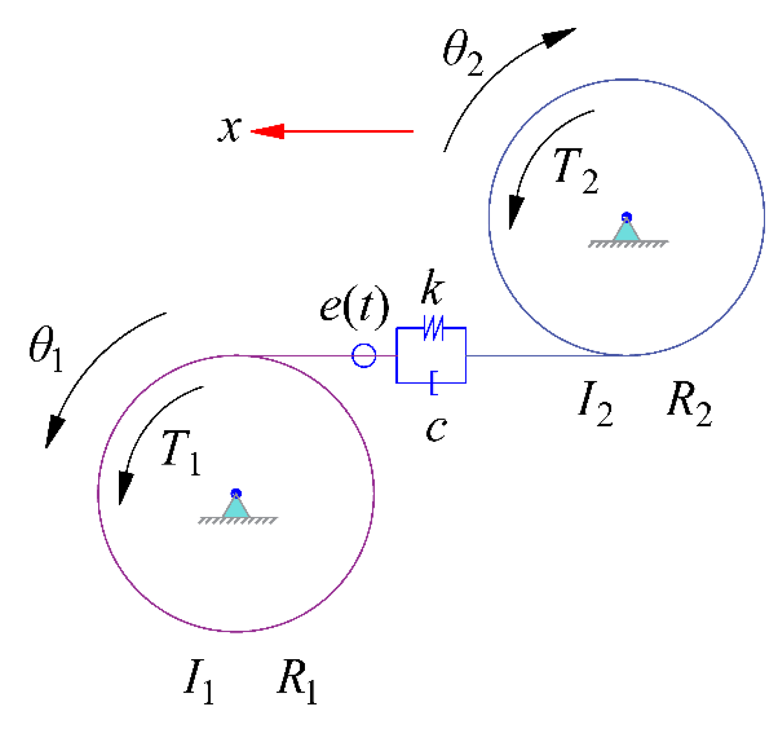
2.1. Establishment of the Dynamic Model of the Nonlinear Gear Systems

Based on the efficient path integration method proposed by Di Matteo, this paper further verifies the relatively complex system, introduces the nonlinear gear system into this theoretical framework, and uses this system to verify and analyze the accuracy and feasibility of this method. Based on the above theory, a nonlinear gear system dynamics model is established in this paper. The model of the nonlinear gear system is shown in Figure 1.
For a nonlinear gear system, the vibration differential equation of the system can be established as:
I 1 θ ¨ 1 + c R 1 ( R 1 θ ˙ 1 R 2 θ ˙ 2 e ˙ t ) + k R 1 f ( R 1 θ 1 R 2 θ 2 e t ) = T 1 I 2 θ ¨ 2 + c R 2 ( R 1 θ ˙ 1 R 2 θ ˙ 2 e ˙ t ) + k R 2 f ( R 1 θ 1 R 2 θ 2 e t ) = T 2
where I 1 and I 2 are the moments of inertia of the driving wheel and the driven wheel, respectively; R 1 and R 2 are the base circle radii of the driving wheel and the driven wheel, respectively; θ 1 and θ 2 are the torsional vibration displacements of the driving wheel and the driven wheel, respectively; T 1 and T 2 are the torques acting on the driving wheel and the driven wheel, respectively; c and k are the meshing damping and meshing stiffness of gear meshing, respectively; and e represents the comprehensive meshing error of gear transmission.
For the convenience of calculation, we perform dimensionless processing on the nonlinear gear system model in Formula (1). Firstly, a generalized coordinate system for the relative displacement of gear meshing is defined [30,31]:
x = R 1 θ 1 R 2 θ 2 e t
Taking the derivative of x gives the following:
x ˙ = R 1 θ ˙ 1 R 2 θ ˙ 2 e ˙ t
For the linear combination of the two equations, let I eq be the equivalent moment of inertia (after merging and simplification), and the system is equivalent to a single-degree-of-freedom system:
I e q x ¨ + c x + k f x = T e q t
where the excitation force at the right end comes from the torque T 1 , T 2 , or is equivalently simplified as a combination of periodic excitation and average torque:
T e q t = T m + T a cos ω n t
Then introduce dimensionless variables:
x = b ¯ x 1
where b represents the tooth side clearance, with units typically in meters or radians, which is used to construct the threshold range of the nonlinear force function. b ¯ is the normalized clearance width, which, together with x, is used to define the piecewise function f x .
τ = ω n t
where   ω n = I e q / k   is the dimensionless excitation frequency.
d d t = ω n d d τ , d 2 d t 2 = ω n 2 d 2 d τ 2
The simplified dynamic equation is as follows:
I e q x ¨ + c x ˙ + k f x = T m + T a cos ω n t
Substituting the above dimensionless variables yields the following:
b ¯ I e q ω n 2 x ¨ 1 + c b ¯ ω n x ˙ 1 + k f b ¯ x 1 = T m + T a cos ω n t
Divide both sides of the equation by k b ¯ to obtain the following:
x ¨ 1 + 2 ζ x ˙ 1 + f x 1 = F m + F a cos ω n t
where ζ = c / 2 k I e q is dimensionless damping, F m = T m / k b ¯ is the dimensionless average excitation term, representing the steady-state part of the external excitation or input torque, and F a = T a / k b ¯ is the dimensionless excitation amplitude, representing the amplitude of the external periodic excitation torque.
Based on the above dimensionless process, the dynamic equation of the dimensionless system is obtained as follows:
x ˙ 1 = x 2 x ˙ 2 = F m + F a cos ω n t 1 ε cos ω n t f x 1 2 ζ x 2
f x = x b ¯ , x > b ¯ 0 , b ¯ x b ¯ x + b ¯ , x < b ¯

2.2. Solution of Probability Density Evolution

The probability density evolution method (PDEM) [32] is often used to analyze the probabilistic behavior of stochastic dynamical systems. By solving the conservation equation of probability density in the given reduced space, we directly obtain the variation in the probability density function (PDF) of the system response over time. The core idea is to directly track the evolution of probability density through deterministic partial differential equations. The core formula is as follows:
d X t d t = f X , t , ξ
where ξ is a random variable, f X , t , ξ is the function corresponding to the random variable, X t is the random process vector, and t is the response time. The joint probability density   p x , ξ , t satisfies the conservation equation:
p x , ξ , t t + f X , t , ξ x p = 0
where x p is the gradient of the probability density   p x , ξ , t in the reduced space.
For the solution of the above-mentioned partial differential equations, the main methods include the finite element method, the path integral method, and the finite difference method. Among them, the path integral method is a way to obtain the evolution of the probability density function (PDF) by integrating the trajectories of the system. This method is applicable to the Markov process under the influence of Gaussian white noise and provides a strict mathematical framework for the evolution of the probability density of nonlinear stochastic systems. In view of this, combined with the urgency of the study on the probability density evolution of nonlinear stochastic systems under the influence of white noise, this paper adopts a path integration method to construct a theoretical framework for solving the probability density evolution equation and reliability.

2.2.1. Markov Processes

Let there be a random process X ( t ) , if for the next arbitrary time series t 1 < t 2 < < t n , under the condition of a given random variable X t 1 = 1 , X t 2 = 2 , , X t n 1 = x n 1 , the distribution of X t n = x n can be expressed as F t n , t 1 , t 2 t n 1 x n | x 1 , x 2 x n 1 = F t n t n 1 x n | x n 1 . Then X ( t ) is called the Markov process [25]. A Markov process is a mathematical model used to describe the random changes in a system between different states. Its key feature is the absence of aftereffect, that is, the state of the system at a certain moment only depends on the state at the previous moment and has nothing to do with the state at an earlier moment. This means that the future state of the system is only related to the current state, and has nothing to do with how the system reaches the current state.

2.2.2. Transition Probability Density Equation

If the nonlinear vibration system can be transformed into the ITO equation in the following form:
d z t = f z t , t + G ¯ z ( t ) , t d W t
The solution z ( t ) of this equation is a typical Markov process, z ( t ) is the n-dimensional state vector, and the transition probability density of z ( t ) is p z | z ¯ .
In the stochastic excitation modeling, the Gaussian white noise excitation ξ t is described by the Wiener process differential d W t , satisfying ξ t d t = d W t , d W t N 0 , d t , where d W t represents the increment of the Wiener process within an infinitesimal time   d t , satisfying the condition of an independent normal distribution and a variance of   d t .
The transfer probability density has the following properties:
R n p z z ¯ d z ¯ = 1
The initial condition of this formula is lim   t 0 p ( z   |   z ¯ ) = δ ( z z ¯ ) , δ is a Dirichlet function, z ¯ is an n-dimensional random variable independent of W t , and the boundary condition is as follows:
p ( z z ¯ ) | z = 0
Thus, the calculation method of the probability density evolution function is obtained as follows:
p Z , k + 1 z = p z z ¯ p Z , k 0 z ¯ d z ¯

2.3. Laplace Asymptotic Expansion Method

2.3.1. Laplace Asymptotic Expansion Method for Solving Joint Probability Density

It can be deduced from the previous section that for solving the evolution process of probability density using the traditional path integration method, its iterative formula can be expressed as follows:
p Z , k + 1 z = p z z ¯ p Z , k z ¯ d z ¯
where the transition probability density p z z ¯ usually involves high-dimensional integrals. Especially for nonlinear systems excited by Gaussian white noise, the direct calculation of integrals is extremely costly. Therefore, it is necessary to approximate the integrals and process the continuous integrals into a discretized format to reduce the computational load.
Based on this, this paper combines the efficient path integration method proposed by Di and introduces the Laplace asymptotic expansion method to process the integrals [27]. The core idea of this method is to find the extreme point z ¯ * of the integral kernel p z z ¯ p Z , k z ¯ and perform Taylor expansion near this point to approximate the integral as an analytical expression, thereby avoiding numerical integration.
First of all, assume that under a short time step size Δ t , the conditional probability density function of the system response follows a Gaussian distribution. Define the logarithmic form of the integrand and convert the integral to the exponential form:
p Z , k + 1 z e 1 q g z , z ¯ p Z , k z ¯ d z ¯
where g ( z , z ¯ ) is a function constructed by the system dynamics equation.
Furthermore, it is necessary to identify the extreme points of p z z ¯ p Z , k z ¯ , that is, the point where g ( z , z ¯ ) is the smallest. The solution formula is as follows:
g z , z ¯ z ¯ z ¯ = z ¯ * = 0
After obtaining the extreme points, perform the second-order Taylor expansion of g ( z , z ¯ ) at the extreme point z ¯ * , and obtain the following:
g z , z ¯ g z , z ¯ * + 1 2 z ¯ z ¯ * T g I I z , z ¯ * z ¯ z ¯ *
where g I I z , z ¯ * = 2 g ( z , z ¯ ) 2 z ¯ z ¯ 2 = z ¯ * is the Hessian matrix, which is represented by g ( z , z ¯ ) . Substitute the expansion into the integral to obtain the Gaussian integral form:
p Z , k + 1 z e 1 q g z , z ¯ * e 1 2 q z ¯ z ¯ * T g I I z ¯ z ¯ * p Z , k z ¯ d z ¯
By using the Gaussian integral formula, the following is finally obtained:
p Z , k + 1 z 2 π n det g I I / q e 1 q g z , z ¯ * p Z , k z ¯ * + q 2 Tr g I I 1 p Z , k I I z ¯ *
For a single-degree-of-freedom system, it is simplified as follows:
p Z , k + 1 z 2 g I I e λ q g z , z ¯ * p ˜ k + q 2 λ g I I p ˜ k I I
where
p ˜ k = p Z z 1 z ¯ 2 * Δ t , z ¯ * , t k
p ˜ k I I = 2 p Z , k z 1 z ¯ 2 Δ t , z ¯ 2 z ¯ 2 2 z ¯ 2 = z ¯ *
The Laplace asymptotic expansion method approximates the Gaussian integral through extreme point expansion, converts the high-dimensional numerical integral in the path integral into analytical calculation, significantly improving the efficiency of random response analysis in nonlinear systems. When dealing with piecewise nonlinearity and time-varying excitation, the accuracy is maintained through dynamic derivative adjustment, thereby avoiding complex integration.

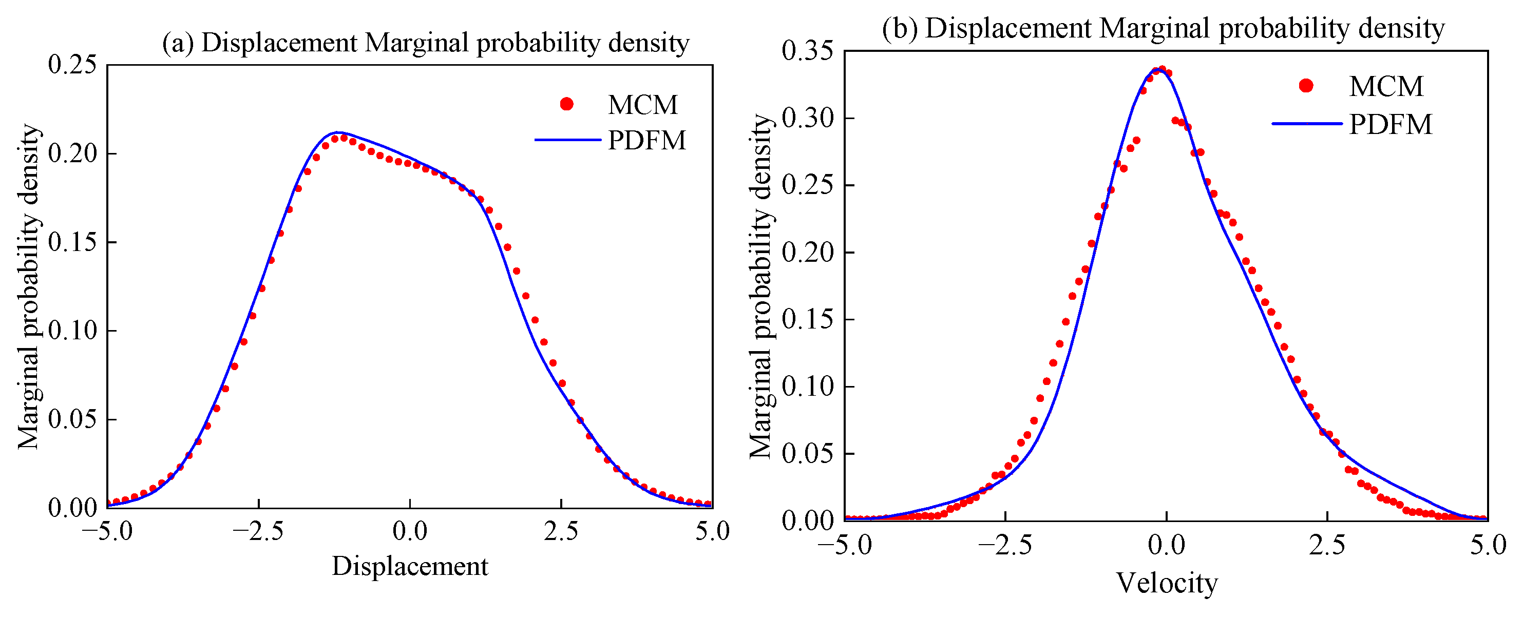
2.3.2. Edge Probability Density

Based on the above-mentioned efficient path integration method, this paper further improves the theoretical framework and expands the applicable objects of this method. First of all, for the known joint probability density, we can calculate the edge probability density of the sum of the two directions of the reduced space. The edge probability density is the dimensionality reduction result of the joint probability density, and the influence of other variables is eliminated through integration. For the joint probability density function p X X ˙ x , x ˙ of the system response X t and its derivative X ˙ t , the edge densities are, respectively:
p X x = p X X ˙ x , x ˙ d x ˙ p X ˙ x ˙ = p X X ˙ x , x ˙ d x
After discretization, the following can be obtained:
p X x i = j = 1 N x ˙ p x i , x ˙ j Δ x ˙ p X ˙ x ˙ j = i = 1 N x p x i , x ˙ j Δ x
where Δ x and Δ x ˙ are the grid step sizes, corresponding to the discrete approximations of the continuous integral, and N x and N x ˙ are the number of grids in the directions of x and x ˙ , respectively. An edge density solution reduces the dimension of high-dimensional joint PDF, intuitively reflecting the statistical characteristics in a single direction and providing evidence for reliability analysis.

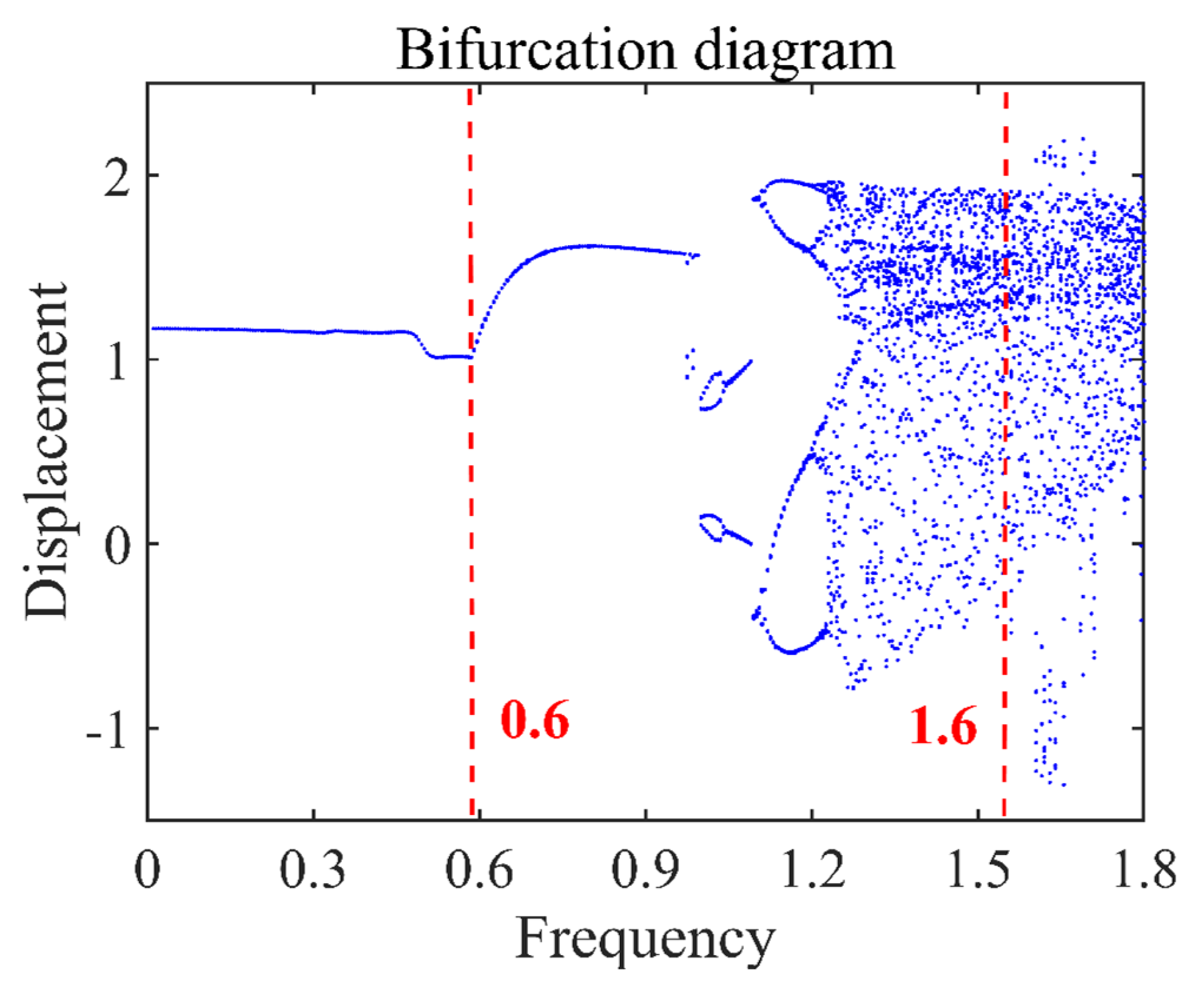
2.4. Evolution Process of Probability Density Under Different Response States

Based on the above theories of probability density evolution and reliability solution, combined with the established dynamic model of the nonlinear gear system, the probability density evolution characteristics and reliability of the nonlinear gear system under different states under the influence of white noise excitation are further analyzed and studied. Firstly, the dynamic characteristics of the nonlinear gear system are studied. The single-period response and chaotic response parameters of the system are selected. The system parameters are set as F m = 1 , F a = 0.5 , ζ = 0.02 , ε = 0.2 , and b = 1 , and ω n = 0 2 is selected. The Runge–Kutta method is used to solve the system, and the bifurcation diagram of the system during the process of dimensionless excitation frequency ω n variation is drawn.
Figure 2 shows the bifurcation diagram of the displacement response of the system with the change in the dimensionless excitation frequency. It can be seen from the figure that under the influence of the dimensionless excitation frequency, the displacement response of the system transitions from a single-period response through multiple bifurcations to a multi-period response and then enters a chaotic response state. Specifically, the system is in a relatively stable range in the single-period response, and its vibration amplitude is not large. The reliability of the system is relatively high. However, as the dimensionless excitation frequency of the system gradually increases, the system gradually tends to an unstable state and continuously transitions to the chaotic response interval. This dynamic state provides a new idea for the reliability analysis of the system, that is, the single-period response state and the chaotic response state of the system can be selected for analysis.
Figure 3a,b show the time-domain graphs of the system at dimensionless excitation frequencies ω n = 0.6 and ω n = 1.6 , respectively, which reflect the variation in the system’s displacement response over time. The bifurcation diagram represents the variation trend of the displacement response with the dimensionless excitation frequency ω n at the same time, and the time-domain diagram represents the variation trend of the displacement response with time under the same dimensionless excitation frequency ω n . Both analyze the response status of the system from different perspectives, respectively. By combining the bifurcation diagram and the time-domain diagram, it can be seen that at time ω n = 0.6 , the system is in a single-cycle response state, while at dimensionless excitation frequency ω n = 1.6 , the system is in a chaotic response state. Therefore, the system was analyzed at dimensionless excitation frequency ω n = 0.6 and ω n = 1.6 , respectively to study the evolution of the probability density and reliability of the system in the periodic response state and the chaotic state.

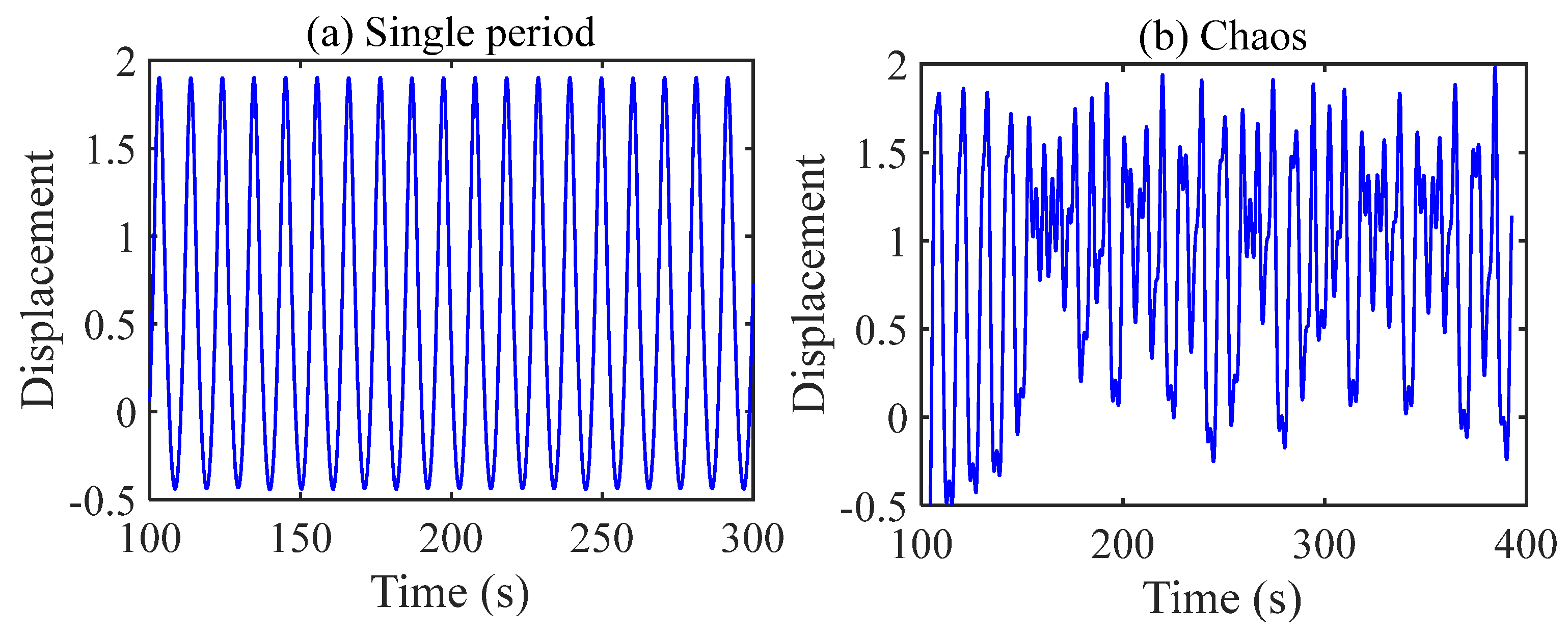
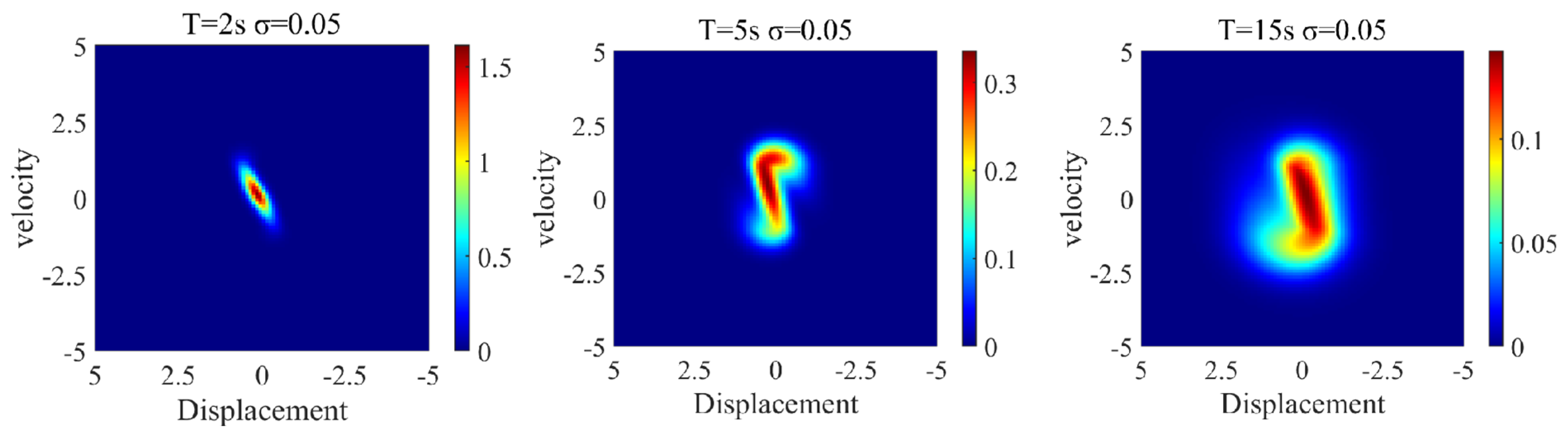
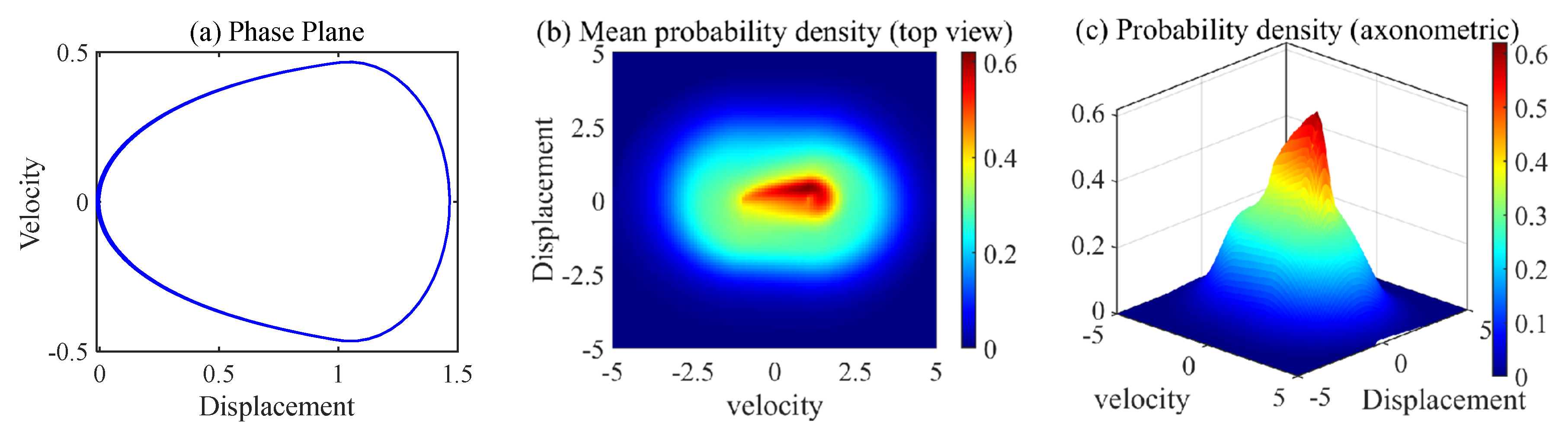
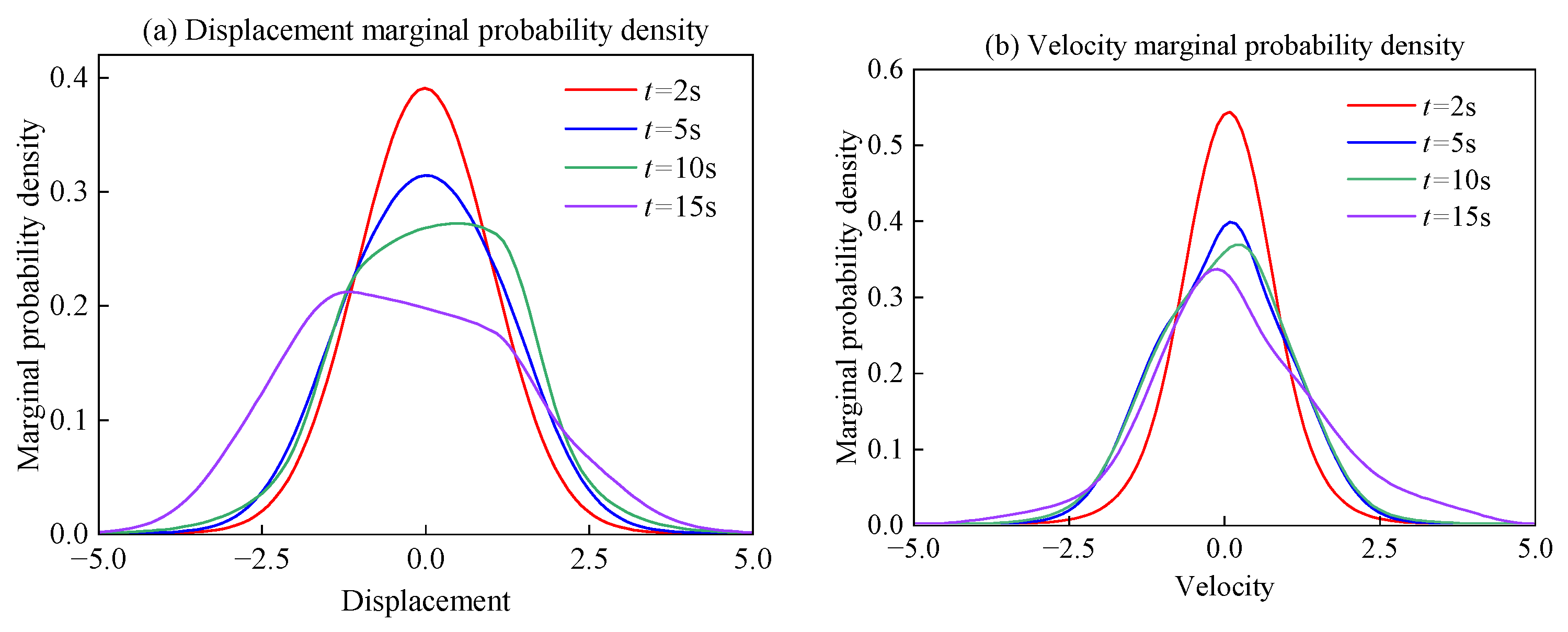
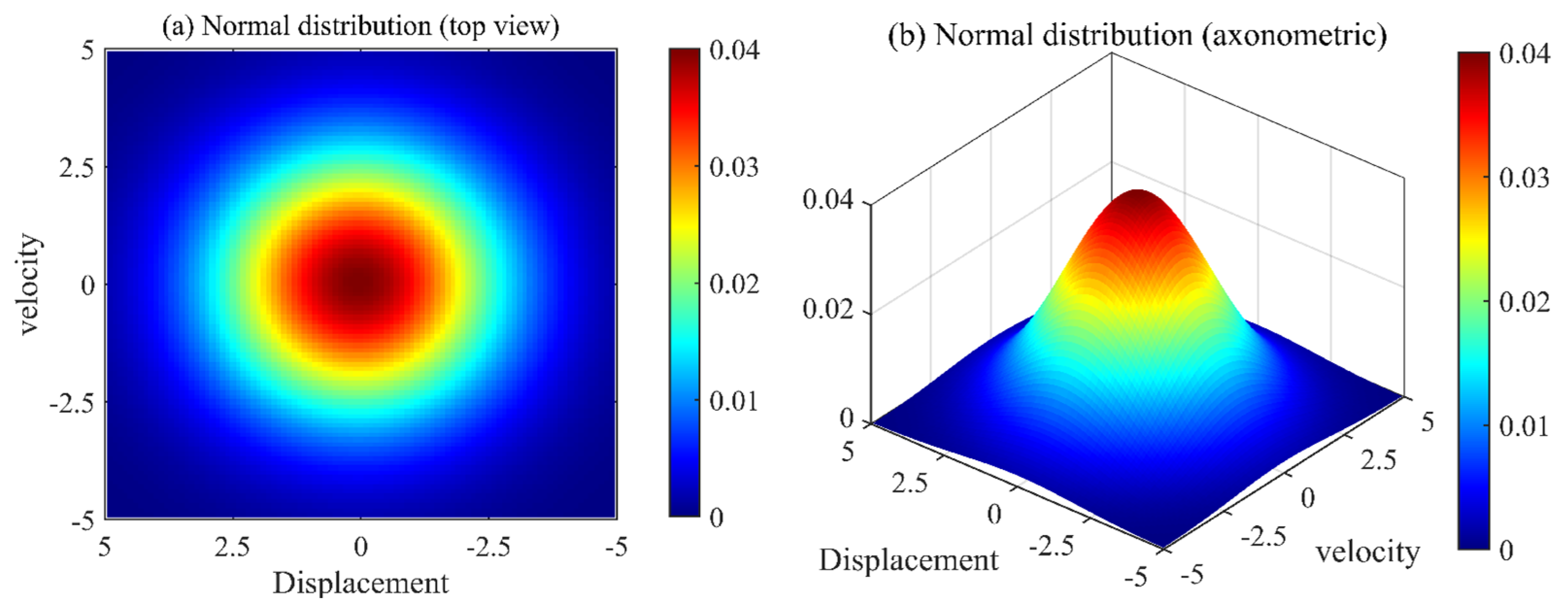
2.4.1. Probability Density Evolution Analysis of Nonlinear Gear Systems Under Periodic Response

To verify the numerical accuracy and algorithm reliability of the established model, this research examines comparative numerical experiments with the Monte Carlo method. Firstly, set the system parameters as: dimensionless excitation frequency ω n = 0.6 , ζ = 0.02 , ε = 0.2 , and other parameters as F m = 1 , F a = 0.5 , and b = 1 . Then apply Gaussian white noise excitation with spectral density σ = 0.05 , and the simulation duration T = 5 s. On the Intel Core i9-13900HX 13th-generation processor platform (Intel, Santa Clara, CA, USA), the Monte Carlo simulation method (the sample size of 1 × 10 3 ) and the algorithm in this paper were adopted for the structural reliability analysis, respectively, as shown in Figure 4.
Figure 4 verifies the solution accuracy of this method by comparing the Monte Carlo method (MCM, red discrete points) with the probability density evolution method proposed in this paper (PDFM, blue continuous curve). The horizontal axes of the velocity distribution are, respectively, the system displacement reduction space (−5.0 to 5.0) and the velocity reduction space (−5.0 to 5.0), while the vertical axes are the corresponding edge probability densities (0.00–0.25 and 0.00–0.35).
In the displacement probability density distribution (Figure 4a), the curve shapes of the two methods show significant consistency. The probability density reaches the peak near the displacement zero point (approximately 0.22), and then shows a symmetrical attenuation trend on both sides. The coincidence degree between the discrete points of MCM and the continuous curve of the method proposed in this paper indicates that the method proposed in this paper can accurately capture the displacement distribution characteristics of the system.
For the velocity probability density distribution (Figure 4b), the curve shapes of the two methods also show significant consistency: the peak positions are basically coincident, and the diffusion to both sides are also basically consistent.
From the perspective of algorithm performance, the comparison results of the two reveal dual advantages: firstly, the calculation accuracy of the method proposed in this paper can be verified through the statistical results of the Monte Carlo method, indicating that it is applicable to the random response analysis of nonlinear systems; and secondly, the probability density curve of the method proposed in this paper is smooth and continuous, and no oscillation or divergence phenomena occur in traditional numerical methods when the excitation complexity increases, confirming its numerical stability and robustness.
Furthermore, this section explores the evolution law of the probability density of nonlinear gear systems in Gaussian white noise interference under periodic response. Set the system parameters as the dimensionless excitation frequency ω n = 0.6 , damping ratio ζ = 0.02 , and nonlinearity coefficient ε = 0.2 , and apply white noise excitation of intensity σ = 0.05 . The probability density distribution of the system in the displacement-time velocity phase space at different times ( T = 2   s , 5   s , 15   s ) was obtained through numerical methods, as shown in Figure 5.
Based on the probability density evolution characteristic image shown in Figure 5, it can be known that the nonlinear gear system presents significant non-equilibrium statistical characteristics in the periodic state. The specific manifestations are as follows: Firstly, the spatial distribution pattern of the system probability density function undergoes significant changes. Its high probability density region gradually spreads from the localized centralized distribution at the initial moment to the peripheral region of the phase space, and its diffusion range expands to nearly three times the initial state. Meanwhile, the peak of the system probability density shows a monotonic attenuation characteristic, continuously decreasing from 1.5 (normalized unit) at T = 2 s to 0.14 at T = 15 s, with a relative decrease of more than 90%. This reveals the redistribution law of the system energy in the phase space.
When the system evolves to T = 50 s, as shown in Figure 6, statistical characterization of the dynamic behavior and probability density evolution within the time interval 40 50   s reveals that the phase plane trajectory is structurally significantly consistent with the high-probability regions ( P D F > 0.5 ) of the average probability density distribution, but there are also widely distributed intermediate probability regions ( 0.2 < P D F 0.5 ) simultaneously in the probability density image. This morphological similarity at the macroscopic scale and the difference in microscopic features jointly indicate that the dynamic response of the system presents typical stochastic-deterministic mixed characteristics. Among them, Gaussian white noise excitation dominates the transient dynamic behavior, while the nonlinear characteristics of the system are characterized by the structure of the probability density distribution in the steady-state stage. This phenomenon indicates that the system still has the ability to maintain its essential nonlinear characteristics in a noisy environment, and the influence of white noise excitation is mainly reflected in the medium-density region (the cyan region in the figure).
Based on this, the edge probability densities of displacement and velocity were further calculated as shown in Figure 7.
Figure 7a shows the evolution law of the displacement edge probability density distribution over time in a nonlinear gear system, and Figure 7b shows the evolution law of the displacement edge probability density distribution over time in a nonlinear gear system. The four-color curves of red ( t = 2   s ) , blue ( t = 5   s ) , green ( t = 10   s ) , and purple ( t = 15   s ) in the figure, respectively, present the spatial distribution characteristics of probability density at different times. It can be seen from the figure that the peak value of the probability density continuously decreases from 0.4 at t = 2   s to 0.23 at t = 15   s , corresponding to the joint probability density, and the probability density gradually spreads in two directions. Under the combined effect of white noise excitation and nonlinear dissipation, the curve shape of the system gradually evolves from the initial sharp Gaussian distribution to a flat distribution. This further indicates that the edge probability density evolution graph can effectively characterize the stochastic dynamic behavior of complex systems, providing a methodology for multi-dimensional analysis of probability density and system reliability.
Secondly, in order to better study the influence of white noise above the system on the evolution of probability density, this study adopts the control variable method to systematically explore the nonlinear influence mechanism of white noise intensity on the evolution of probability density. The influence of white noise on the system is demonstrated by setting three gradients σ = 0.01 (low), 0.05 (medium), and 0.07 (high).
As shown in Figure 8, the analysis of the transient probability density distribution characteristics indicates that during the evolution of the white noise excitation intensity parameter σ 0.01 , 0.07 , the probability density distribution of the nonlinear gear system in the periodic motion phase space presents significant evolution features. With the monotonically increasing white noise intensity parameter σ, the probability density shows an obvious radial diffusion effect, which is specifically manifested as follows: the high-density area of the probability distribution continues to expand, and the area of the high-probability density area increases several times. Secondly, the peak of the probability density shows a monotonic attenuation characteristic, and the peak’s maximum reduction reaches 72.2%. This phenomenon reveals the evolution characteristics of the steady-state probability density of the system under the excitation of white noise from the perspective of stochastic dynamics. The degradation of this dynamic characteristic will cause the decline in the nonlinear characteristics of the system and significantly increase the risk of system failure.

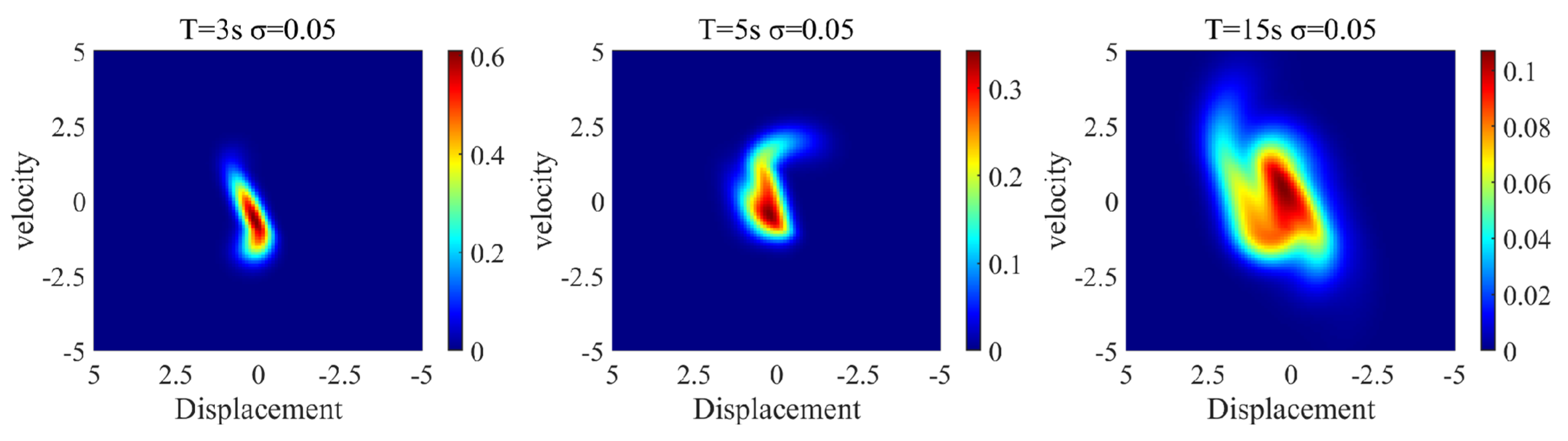
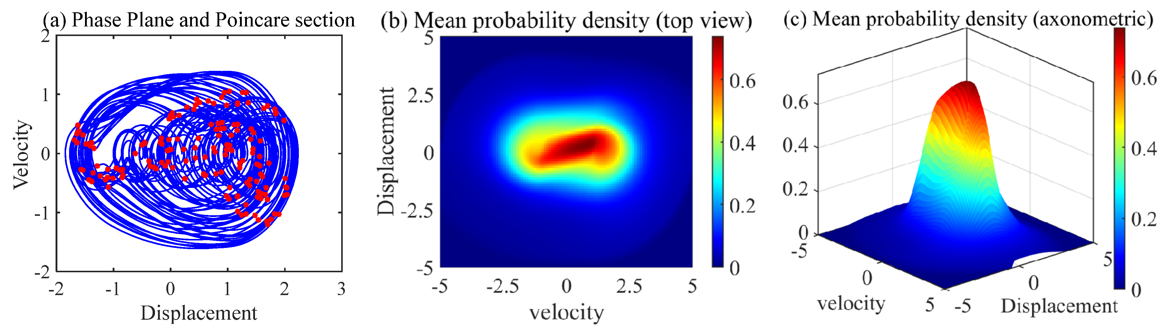
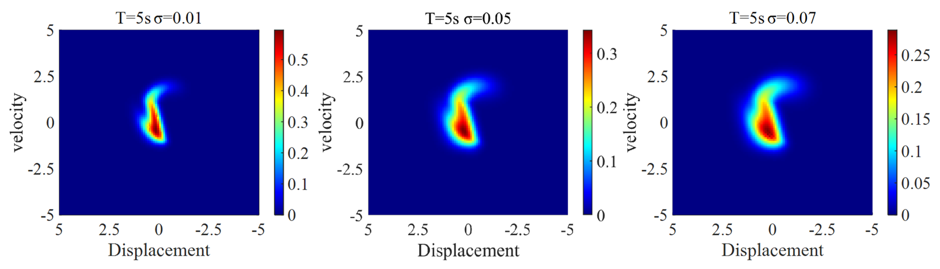
2.4.2. Probability Density Evolution of Nonlinear Gear Transmission Systems Under Chaotic Response

Take the dimensionless excitation frequency ω n = 1.6 , damping ratio ζ = 0.02 , nonlinearity coefficient ε = 0.2 , and other parameters F m = 1 , F a = 0.5 , and b = 1 , and apply Gaussian white noise excitation with spectral density σ = 0.05 . The simulation duration is T = 5 s. The evolution process of the probability density in the chaotic state is obtained as shown in Figure 9.
To reveal the time-varying influence law of the chaotic effect on the evolution mechanism of probability density, this study drew the probability density distribution maps at three characteristic moments of T = 3 s, 10 s, and 15 s under the condition of noise intensity σ = 0.05, as shown in Figure 9. Numerical analysis shows that the probability density distribution in the reduced space presents significant non-stationary evolution characteristics. Its probability density is affected by the dynamic characteristics of the chaotic attractor of the system and shows a more complex trajectory during the evolution process. Quantitative evolution analysis shows that when the system evolution time extends from T = 3 s to T = 15 s, the probability density distribution produces a significant diffusion effect, which is specifically manifested as follows: the area of the high probability density region expands and the peak of the probability density decays. The gradual weakening of this probability density aggregation effect essentially stems from the effect of chaotic attractors on the instability of the phase space structure. Furthermore, the evolution of the system in this response state is much more intense than that in a single period. This also indicates the instability of the system in the chaotic response state, and this instability will also lead to an increase in the failure probability.
Similarly, calculate the average probability density of the system, take the average probability density of the system within 90–100 s, and draw its probability density graph.
Figure 10 reveals the dynamic characteristics of the nonlinear gear system under the excitation of white noise within a time range of 90 to 100 s. Figure 10a shows the displacement-time phase plane trajectory (blue line) and the Poincaré section (red dot), presenting a typical aperiodic fractal structure. At this point, the system motion has deviated from the simple periodic oscillation and entered the chaotic response state. In the top views of the probability density shown in Figure 10b,c, the yellow–red high-probability regions present an ellipsoidal diffusion form. By comparing with the structures of the phase plane and the Poincaré section, it is found that at this time, the steady-state probability density still has a certain gap from the phase plane trajectory and the Poincaré section of the system, and its shape is closer to the Poincaré section, indicating that the motion of the system is greatly affected by the excitation of white noise. The characteristics exhibited by the system in this state, which are “neither completely regular nor completely random”, and the complexity of the trajectory indicate that it is both affected by white noise excitation and to some extent reflects the nonlinear response.
However, compared with the periodic response state, the system in this state shows more of the random response state. This transformation of dynamic characteristics indicates that in the chaotic state, the system is in a more unstable state, and provides a dynamic explanation for the abnormal failure phenomenon of the nonlinear gear system in a specific parameter domain, providing a theoretical basis for the subsequent reliability analysis.
Secondly, calculate the edge probability density of the system in this state. Take the iteration time as T = 5 s, and obtain the edge probability density distributions of the displacement and velocity of the system, respectively.
Figure 11a shows the evolution law of the displacement edge probability density distribution in the studied system over time, and Figure 11b shows the evolution law of the displacement edge probability density distribution in the studied system over time. The two figures show the law of the evolution of the probability distribution characteristics of displacement and velocity in the dynamical system over time.
In Figure 11a, the probability density curves at the four-time nodes all present a unimodal form, but their characteristics have significant time-varying laws: at the initial moment t = 2   s (red curve), a sharp peak (density 0.34) forms at the displacement x = 0 . As time goes by to t = 15   s (purple curve), the peak height decreases by approximately 45% and the distribution widens, indicating that the uncertainty of the system displacement gradually increases.
Figure 11b shows a more complex evolutionary pattern. At t = 2 s (red curve), a highly concentrated probability distribution (peak density 0.54) is formed near v = 0 . As time progresses, the center of the distribution shifts significantly and its peak gradually decreases. The comparative analysis of the two figures reveals that there exists significant asymmetry in the probability evolution of the system in different dimensions of the phase space, and there is an offset phenomenon in the velocity dimension. This also indicates that the system has more complex dynamic behaviors in the chaotic response state, which also confirms that the chaotic response state has greater uncertainty.
Next, the probability density of the system under the chaotic response state under the influence of different Gaussian white noises is further studied. The Gaussian white noise intensifications with three gradients of σ = 0.01 (low), 0.05 (medium), and 0.07 (high) are set for comparative analysis. The results are shown in Figure 12.
The numerical simulation results show that as the Gaussian white noise excitation intensity parameter σ increases from 0.01 to 0.07, the probability density function of the gear system presents a significant evolution law. The specific manifestations are as follows: the probability density function shows a diffusion trend in all directions of the reduced space, and its peak shows a decreasing trend. It is worth noting that when the system is in a chaotic response state, the spatial diffusion degree of its probability density distribution is significantly reduced compared with the periodic response state. This indicates that the enhanced intrinsic dynamic instability of the system supposes the perturbation effect of Gaussian white noise to a certain extent. This phenomenon reveals that in the chaotic motion state of the nonlinear system, its own instability has a certain shielding effect on Gaussian white noise.
In this section, through the theory of probability density evolution and combined with numerical simulation methods, the statistical characteristics of nonlinear gear systems in periodic and chaotic response states are systematically studied, revealing the coupling effect between white noise excitation and the nonlinear dynamics of the system. The specific manifestations are as follows: in the periodic response state, the high-probability area gradually spreads outward from the initial concentrated state to about three times the initial size, and the peak value continuously decreases, indicating that the system response is redistributed in the reduced space over time. Secondly, in this state, the system presents a stochastic-deterministic duality: the macroscopic phase trajectory is consistent with the average probability density structure, but there are differences in the microscopic statistical characteristics. This indicates that noise excitation dominates the transient behavior, while the nonlinear characteristics of the system are characterized by the steady-state probability density structure. In the chaotic response state, the evolution of probability density is affected by chaotic the attractors, presenting a more complex diffusion pattern. Its phase plane trajectory and Poincaré section are not completely consistent with the probability density distribution pattern, revealing that the system is in a state were Gaussian white noise excitation and nonlinear response act together. Thirdly, the enhancement of white noise has a limited promoting effect on the diffusion of probability density. The instability of chaos itself becomes the dominant factor, resulting in a further reduction in the reliability of the system.
In conclusion, noise has a significant impact on system evolution in the periodic state, while in the chaotic state, dynamic instability dominates and the noise effect is relatively weakened. This indicates that both states have accumulated failure risks, but the mechanisms are different: the periodic state results from energy dispersion caused by noise, while the chaotic state results from the instability of the attractor structure.

3. Reliability Analysis of Nonlinear Gear Systems

3.1. Adaptive Gauss–Legendre Method

A challenging issue in the numerical calculation of the probability density of nonlinear dynamics is the nonlinear variation in its state. In linear system problems, this can be overcome by determining two points within one time step and dividing them into two different sub-steps. However, in the corresponding nonlinear stochastic dynamics analysis, it is difficult to guarantee the accuracy of this method in solving the probability density. Moreover, in the efficient path integration method proposed by Di, the Laplace asymptotic expansion method it uses has a relatively high computational complexity and a high cost in the process of calculating reliability. Therefore, in this paper, a new adaptive integration method is adopted. Compared with the fixed-point Gauss–Legendre method, it reduces the numerical error and improves the solution accuracy.

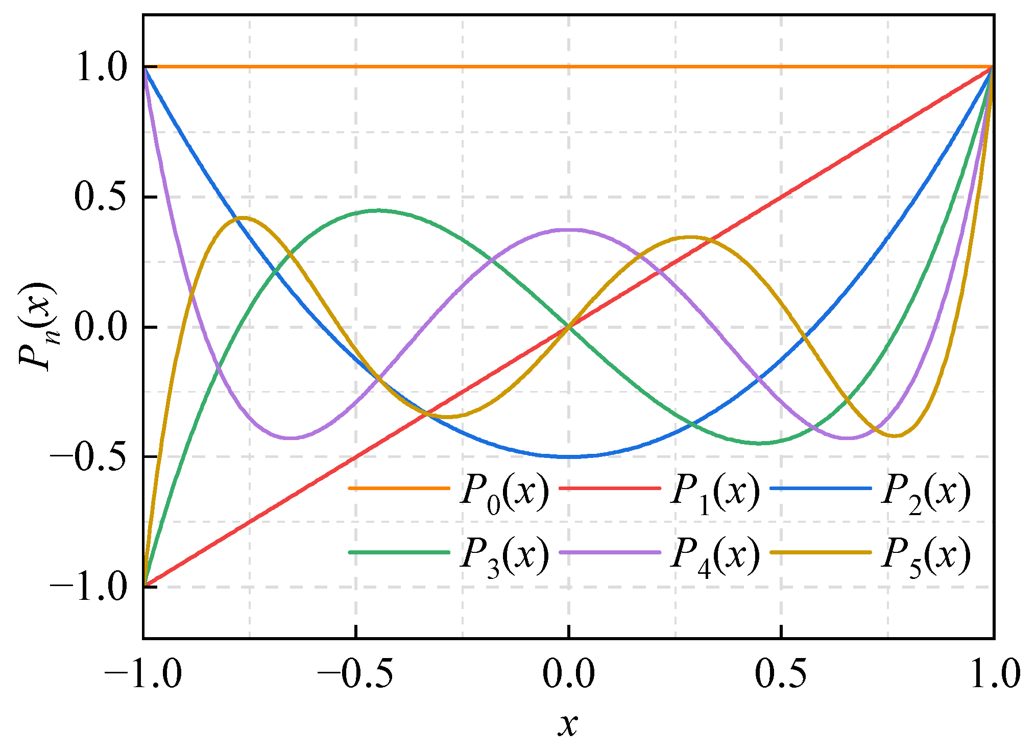
3.1.1. Gauss–Legendre Product Formula

Legendre polynomials are a set of orthogonal polynomials defined on an interval 1 , 1 , denoted as P n x , and that satisfy the Legendre differential equation:
1 x 2 d 2 y d x 2 2 x d y d x + n n + 1 y = 0
where n is a non-negative integer, representing the degree of the polynomial. When n is an integer, the equation has a polynomial solution on the interval 1 , 1 , which is called the Legendre polynomial and is denoted as   P n x . Legendre polynomials can be directly expressed through Rodriguez’s formula:
P n x = 1 2 n n ! d n d x n x 2 1 n
Its first five order polynomials are shown in Figure 13.
It can be seen from the figure that this family of functions has unique mathematical properties within the interval x 1 , 1 . The first sixth-order polynomial ( P 0 x to P 5 x ) is generated through recursive relations, and its explicit expression shows significant order evolution laws. Specifically, the number of extreme points of each order polynomial within an interval is strictly equal to its order. For example, P 4 x has four extreme points and four real roots, while maintaining the symmetry of even functions, that is, odd-order polynomials are odd functions, and even-order polynomials are even functions.
It is worth noting that Legendre polynomials satisfy the characteristic of orthogonality on the interval 1 , 1 , that is as follows:
1 1 P m x P x d x = 0 , m n , 2 2 n + 1 , m = n .
Each P n x satisfies   P n 1 = 1 and   P n 1 = 1 n . The Gauss–Legendre integral [33] is a numerical integration method. Its core lies in using the roots of the Legendre polynomial as nodes, selecting n nodes x i and the corresponding weights ω i , so that the integration formula i = 1 n ω i f x i holds precisely for the highest (2n−1) degree polynomial, and approximating the integral by the sum of the function values of these points and the corresponding weights. The formula is as follows:
1 1 f ( x ) d x i = 1 n ω i f ( x i )
That is, select certain interpolation points and interpolation weights to approximate the integral value. The expression of the weight value of Gauss–Legendre obtained from the orthogonality condition is as follows:
ω i = 2 1 x 2 P n x i 2
The first four order weights ω i and the corresponding Gaussian interpolation points x i are shown in Table 1, where x i is the Gaussian integral point and ω i is the corresponding weight. For the general interval a , b , we perform a linear transformation to convert it into 1 , 1 .
a b f ( x ) d x i = 1 n ω i f b a 2 x i + b + a 2 b a 2
For the selection of the number of integral points n, the larger n is, the higher the accuracy, but the amount of calculation increases. It is usually selected based on the smoothness of the integrand and the required precision. This method has symmetrical node distribution, positive weights, and good numerical stability. However, as n increases, the amount of calculation increases and the calculation cost also increases. An adaptive Gauss–Legendre integration method proposed in this paper can adaptively adjust the number of integration points according to the error size, saving calculation time while ensuring accuracy.

3.1.2. Adaptive Gauss–Legendre Integration Method

Suppose it is necessary to calculate the integral of function f x over the interval a ,   b , and the error tolerance is set to ε . Calculate the initial integral value using the Gauss–Legendre integration formula:
I 0 = i = 1 n ω i f b a 2 x i + b + a 2 b a 2
where ω i is the weight of the Gaussian integral point. Divide the interval a ,   b into two parts, a ,   c and c ,   b , where c = a + b 2 , and calculate the integral values I 1 and I 2 on the two sub-intervals:
I 1 = i = 1 n ω i f c a 2 x i + c + a 2 c a 2 I 2 = i = 1 n ω i f b c 2 x i + b + c 2 b c 2
By comparing the initial integral value with the integral values of the two sub-intervals, the estimated error is as follows:
error = I 0 ( I 1 + I 2 )
If error < ε , then I = I 1 + I 2 . Otherwise, continue to refine the sub-intervals and apply the above-mentioned adaptive integration method to a ,   c and c ,   b , respectively, until the errors meet the requirements. For the final obtained integral value, it will obtain the corresponding weights based on the number of integral points and the size of the integral interval mentioned above, and normalize the weights. The corresponding probability density value is calculated based on the obtained normalized weights.
Let the total number of intervals be N = 2 k . Each subdivision reduces the error to 1 / 2 2 n + 1 of the original value. Then the global error satisfies the following:
E total ε 1 1 / 2 2 n

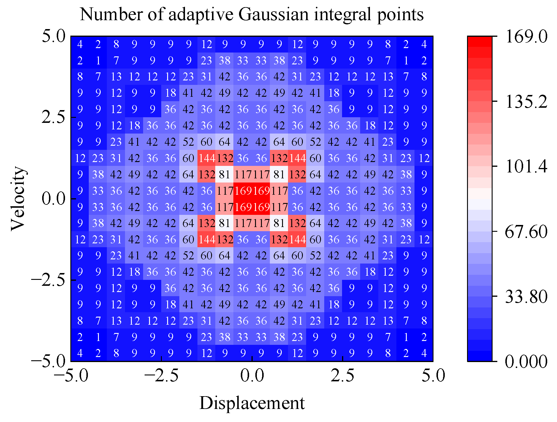
3.1.3. Two-Dimensional Adaptive Gauss–Legendre Integration Method

For two-dimensional integrals, similarly, the two-dimensional integration interval a x , b x × a y , b y can be recursively refined in the x and y directions, respectively. Suppose there is a joint probability density function f x , y , then the initial integral that can be obtained is as follows:
I 0 = i = 1 n j = 1 m ω i ω j f b x a x 2 x i + b x + a x 2 , b y a y 2 y j + b y + a y 2 b x a x 2 b y a y 2
where ω i and ω j are the weights in the x and y directions, respectively.
Define the integral interval in two parts, a x , b x and a y , b y , and calculate the integral value on each sub-interval. Estimate the error using Equation (39) and recursively divide it until the error meets the requirements. This method refines the integration interval recursively and can obtain high-precision integration results on functions with non-uniform distribution. It is very suitable for dealing with complex integration problems.
Taking the two-dimensional standard normal distribution as an example, the adaptive situation of the adaptive integration points is shown in Figure 14.
Figure 14a,b show the top view and axial view of the probability density of the two-dimensional standard normal distribution, respectively. A two-dimensional space is constructed with displacement and velocity as coordinates. The density is the highest in the central red area and gradually decays outward to the blue low-density area. Figure 15 shows the distribution characteristics of adaptive Gaussian integral points corresponding to the two-dimensional standard normal distribution. Each grid in the figure is a reduced space of 1 × 1 , and the numbers within the grids represent the number of Gaussian integral points in this reduced space. It can be seen from the figure that as the probability density value of the two-dimensional standard normal distribution gradually decays from the center to the periphery, the corresponding number of Gaussian integration points also gradually decreases sharply from the dense number of integration points in the central area (red, up to 169 points at the highest) to the periphery (blue, the lowest is close to 0). This indicates that the adaptive method dynamically allocates integration resources based on probability density. In the high-density area, the integration accuracy is improved by increasing the number of integration points, and in the low-density area, the computing cost is saved with fewer integration points. This further proves the accuracy and effectiveness of the method.

3.2. Reliability Indicators Based on Average Crossing Rate

3.2.1. Rice’s Theory and Average Crossing Rate

In the field of engineering reliability, the probability analysis of the system’s dynamic response exceeding the safety threshold is one of the core issues in evaluating system performance. Based on Rice’s theory, this section systematically constructs the mathematical correlation between the average crossing rate and reliability, and discretizes the integral by using the above-mentioned adaptive Gauss–Legendre integration method, thereby simplifying the calculation and solving the final result.
The core of Rice’s theory is to study the statistical characteristics of random processes (such as noise and vibration signals) during Threshold Crossing. For the zero-mean stationary Gaussian process X t , its upward crossing rate above the threshold a (crossing the threshold from bottom to top) is as follows:
λ + a = 1 2 π λ 2 λ 0 exp a 2 2 λ 0
where λ 0 = V a r X t is the variance of the X t . λ 2 = V a r X ˙ t is the variance of the X ˙ t . λ 2 / λ 0 is the root mean square frequency of the process, reflecting the speed of signal change.
According to the stochastic process theory and the concept of crossing rate proposed by Rice, the average crossing rate of the system’s response X crossing the critical value ξ can be calculated by the following formula:
ν X + ξ = 0 p X X ˙ ξ ;   t d s
The above-mentioned adaptive Gauss–Legendre integration method is used to discretize the integral, and the discretization formula of the average crossing rate is obtained as follows:
v X + ξ = k s = 1 K s δ k s 2 l s = 1 L k s c k l s k = 1 K δ k 2 l = 1 L k c k l p X X ˙ ξ , s k l s ; t k l
where L k represents the number of Gaussian integral points, c k l s represents the weights of Gaussian integral points, K represents the number of discrete Spaces, and δ k represents the length of the subspace.

3.2.2. Reliability Theory and Reliability Indicators

Under the theoretical framework of engineering system reliability, reliability, as the core quantitative indicator characterizing the ability of a system to continuously maintain the expected functions within the given operating conditions and time domain, has a mathematical definition that can be formally expressed as follows: Suppose the life T of the system under the specified operating environment constraints is a continuous random variable. Then the reliability function R t of the system within the time interval 0 , t can be defined as the probability measure of the system’s trouble-free operation time exceeding the specified time threshold, specifically as follows:
R t = P X τ Ω s , τ 0 , t
where X τ is a random vector characterizing the system state (such as vibration amplitude, stress-strain, etc.), Ω s is the state safety domain, and P represents the probability.
From the perspective of the time dimension, system reliability can be divided into two forms: transient reliability and cumulative reliability. Transient reliability characterizes the probability that the system maintains a normal operating state within a determined time point t, and can accurately reflect the dynamic reliability characteristics of the system at the microscopic time scale. Cumulative reliability is defined as the joint probability measure of a system continuously satisfying functional constraints within the extended time domain 0 , T . Its form is a decreasing function and it is a core analytical tool in reliability engineering.
The probability density function p x , t of the system state is established based on the probability density evolution equation. The reliability is expressed as the integral of the probabilities within the safety domain Ω s . The calculation formula of the reliability can be expressed as follows:
R t = Ω s p x , t d x
When the system trajectory crosses the failure boundary Γ = Ω s for the first time, it is determined as a failure event. Based on the above theory, the expression for obtaining reliability using the crossing rate can be derived as follows:
R ξ = exp ν X + ξ
Based on Rice’s theory and the adaptive Gauss–Legendre integration method, this section establishes the basic method for solving the reliability of nonlinear gear systems. The average crossing rate model of random processes exceeding the safety threshold was established through Rice’s theory. The continuous integration problem was discretization into an efficient numerical calculation form, and the adaptive Gauss–Legendre integration algorithm was used to dynamically adjust the distribution of integration nodes, significantly reducing the computational complexity of high-dimensional integrals. Next, in accordance with the above theory, this paper will analyze the probability density evolution process and dynamic reliability of the nonlinear gear system.
The process of the method proposed in this manuscript is as follows:
Step 1: Establish the nonlinear dynamic equation (Equation (49)), and obtain the joint probability density p x x ˙ x , x ˙ ; t by solving the probability density evolution equation through Laplace asymptotic expansion;
Step 2: Calculate the displacement edge densities p x x ; t and p x ˙ x ˙ ; t ;
Step 3: Use Rice’s theory combined with the two-dimensional adaptive integration strategy to solve the transient crossing rate v X + ξ ; t ;
Step 4: Obtain the transient reliability and cumulative reliability curves through integration.
The flowchart of the path integration method proposed in this paper for calculating the evolution of probability density and dynamic reliability is shown in Figure 16.

3.3. Gear Reliability Under Different Response States Based on the Evolution of Probability Density

In the previous section, through multi-scale statistical dynamics and probability density evolution analysis, the failure mechanism and evolution process of nonlinear gear systems under different dynamic states were clarified. Next, it is necessary to further explore the reliability of the system under different states.
Firstly, in order to prove the effectiveness of the method proposed in this paper in controlling the time cost, the reliability of the Monte Carlo method (sample size 1 × 10 5 ), the method of solving the probability density using the moment equation (M-PDFM), and the method in this paper (A-PDFM) in solving were compared, respectively. Take the dimensionless excitation frequency ω n = 0.6 , ζ = 0.02 , and ε = 0.2 , and other parameters were F m = 1 , F a = 0.5 , and b = 1 . And apply the white noise excitation of intensity σ = 0.05 . Take the iteration time T = 15 s and calculate the time used, as shown in Figure 17.
It can be seen through comparison that the calculation efficiency of the method proposed in this paper is increased by 84.97% compared with the Monte Carlo method, and by 65.77% compared with the method of solving the probability density using the moment equation, which proves the effectiveness of the method proposed in this paper.

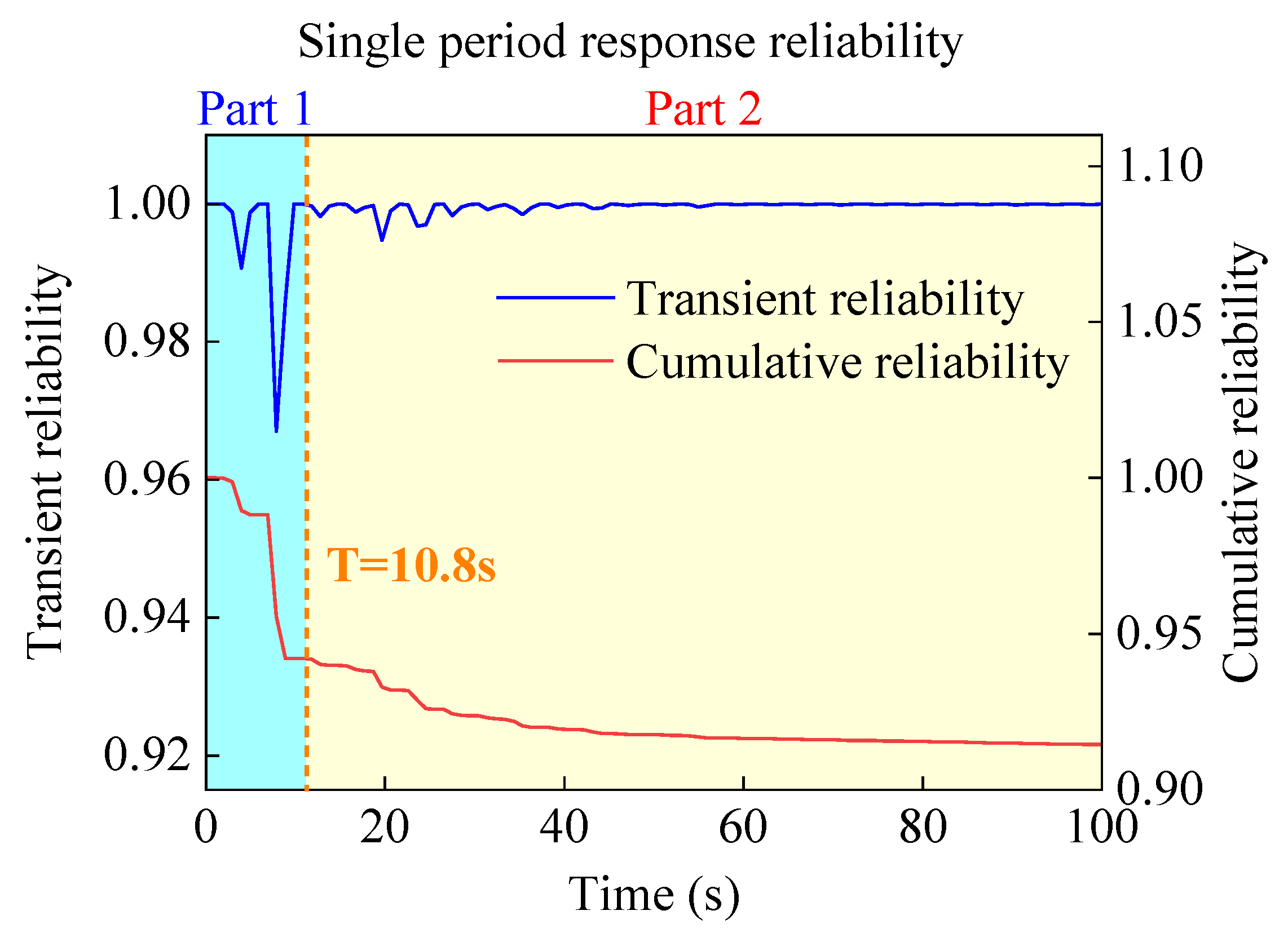
3.3.1. Nonlinear Gear Transmission Systems with Periodic Response

Take the dimensionless excitation frequency ω n = 0.6 , the single-cycle dynamic response of the system. Take the damping ratio ζ = 0.02 , the nonlinearity coefficient ε = 0.2 , and other parameters F m = 1 , F a = 0.5 , and b = 1 . Apply the white noise excitation of intensity σ = 0.05 . Take the response limit value as the dimensionless value 5, and conduct the reliability analysis using Rice’s theory. The transient reliability and cumulative reliability evolution curves shown in Figure 18 reveal the following dynamic characteristics: during the initial operation stage of the system, significant instability phenomena are presented, specifically manifested as a substantial decrease in transient reliability within the t 0 , 10.8   s interval (Part 1) and a steep negative gradient decrease in the cumulative reliability curve. This nonlinear attenuation characteristic stems from the unstable movement of the system in the early stage. As the running time progresses to t > 10.8   s (Part 2), the transient reliability gradually converges to the steady-state value range, and the corresponding cumulative reliability curve also gradually tends to be flat and stable. This two-stage reliability evolution law confirms the phenomenon that the system gradually stabilizes through self-regulation after experiencing the initial transient oscillation.

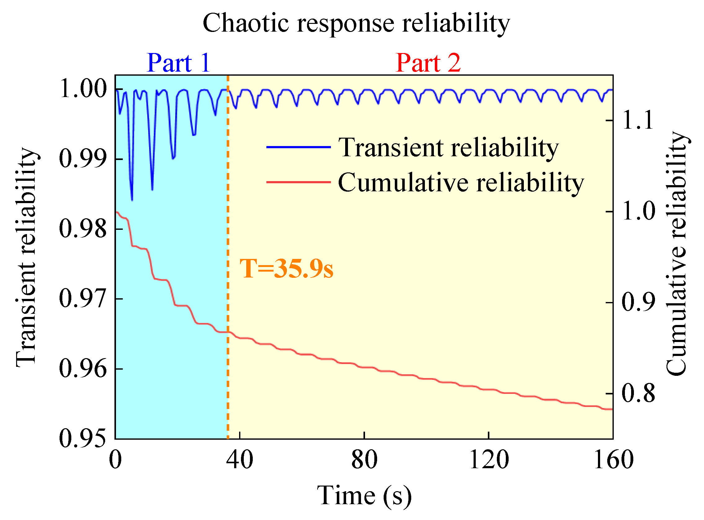
3.3.2. Nonlinear Gear Transmission Systems with Chaotic Responses

Furthermore, take the dimensionless excitation frequency ω n = 1.6 to study the reliability of the nonlinear gear system in the chaotic response state of the system. Similarly, take the ζ = 0.02 , the ε = 0.2 , and other parameters F m = 1 , F a = 0.5 , and b = 1 , and apply the white noise excitation of intensity σ = 0.05 . Its reliability evolution law shows similar convergence characteristics to the dynamic system, as shown in Figure 18. Similarly to the reliability tendency of periodic response gear systems, the transient reliability curve reflects the variation in reliability at each moment and can reveal the dangerous moments of the system.
Compared with the gear system in the periodic response, its cumulative reliability shows more intense initial deterioration characteristics under the chaotic response: within t 0 , 35.9   s (Part 1), the cumulative reliability decreases rapidly, at a faster rate than the single-periodic response, and the time of its initial unstable state is longer. When t = 35.9   s is reached, the cumulative reliability has entered the asymptotic stable zone. However, within the stable range, its decline rate is still larger than that of the single-period response, and its stable value also decreases. The system enters a stable period after t > 35.9   s (Part 2), at which point the fluctuation amplitude of the transient reliability is limited within the range of Δ R < 0.02 . This process further reveals the intense evolution process of high dissipation of the system in the chaotic response state, corresponding to the previous probability density evolution analysis.
Under the periodic response state ( ω n = 0.6 ), the reliability shows a two-stage attenuation characteristic (Figure 18). In the initial stage (0–10.8 s), the probability density diffusion caused by noise (Figure 9, Figure 10, Figure 11 and Figure 12) leads to a rapid decrease in reliability, but in the steady-state stage (t > 10.8 s), the reliability tends to stabilize. This indicates that although the periodic state is affected by noise, the failure risk can be effectively controlled by enhancing the system damping (ζ) or suppressing the intensity of external noise (σ). For example, when σ decreases from 0.07 to 0.01, the attenuation amplitude of the peak probability density decreases significantly (Figure 12), verifying the positive effect of noise suppression on reliability.
Under the chaotic response state (such as ω n = 1.6 ), the system reliability shows a sharp attenuation characteristic (Figure 19). Specifically, the rate of decline of cumulative reliability in the initial stage (0–35.9 s) is much faster than that of the periodic response. This stems from the instability of the phase space structure caused by chaotic attractors, which leads to the exponential amplification of tiny disturbances. At this point, the gear system is in a mixed failure mode of “deterministic chaos dominance-noise assistance”, and its failure risk mainly comes from the dynamic instability of the system itself rather than external noise. Therefore, in engineering design, parameter regulation (such as restriction ω n ) is needed to prevent the system from entering a chaotic state.
Based on the theory of probability density evolution, this section comparatively analyzes the reliability evolution laws of nonlinear gear systems under periodic responses and chaotic responses, revealing the influence mechanism of different dynamic states on the system reliability. Studies show that under periodic response, the system reliability presents a typical two-stage attenuation characteristic-in the initial stage (Part 1), the reliability drops rapidly due to the sharp increase in transient failure rate, while as the system self-regulates and gradually enters the stable stage (Part 2), the cumulative reliability attenuation rate slows down significantly and the transient reliability converges to the steady-state threshold; under chaotic response, the evolution of system reliability shows a more intense dynamic dissipation characteristic. The cumulative reliability decreases at a rate much higher than the periodic response in the initial stage (Part 1), and the stable value of reliability in the stable stage (Part 2) is lower. The fluctuation amplitude of transient reliability increases significantly, confirming the high energy dissipation characteristic of chaotic motion.
This section also verifies the numerical accuracy and algorithm robustness of the proposed method through the comparison between Monte Carlo simulation and the method proposed in this paper. The research conclusion not only clarifies the reliability degradation mechanism of the gear system in the nonlinear dynamic state, but also provides a theoretical basis for the identification of dangerous moments, life prediction and reliability optimization in engineering, corresponding to the above probability density evolution process.

4. Conclusions

This paper proposes a new method for solving the evolution of probability density based on the path integration method, which is used to analyze the evolution of probability density and reliability of nonlinear gear systems under random excitation of Gaussian white noise. By combining the path integration method and the Laplace asymptotic expansion method, an efficient probability density evolution framework was constructed. The system reliability was calculated using Rice’s theory and the adaptive Gauss–Legendre integration method, solving the problem of insufficient accuracy of traditional methods in nonlinear systems. Through research and analysis, the following conclusions were drawn:
(1) For the nonlinear gear system excited by Gaussian white noise, the probability density evolution analysis process has been improved. By studying the synergistic mechanism between the nonlinear dynamic characteristics of the system and the random excitation, the visual representation of the evolution of the phase space probability density was achieved.
(2) The probability density evolution equation under non-stationary random excitation was established, and the Laplace asymptotic expansion method was introduced to solve the high-dimensional integrals.
(3) By using the adaptive Gauss–Legendre integration method and Rice’s theory, a reliability calculation method with an error control strategy is derived. Through the node adaptive algorithm, the quantitative characterization of the failure probability of the first crossing was achieved, improving the calculation efficiency and increasing the calculation accuracy.
(4) Based on the evolution of probability density and the results of reliability calculation, the influence mechanism of different dynamic states on the system reliability is revealed, that is, the reliability change under periodic response is relatively gentle, while the reliability change under chaotic response state is drastic. Verified by Monte Carlo simulation, the method proposed in this paper shows advantages in both computational efficiency and accuracy.
(5) This study reveals the synergistic effect between white noise excitation and nonlinear dynamics, clarifies the failure mechanisms of gear systems under different working conditions, that is, the failure risk under periodic response is mainly external noise, while the failure risk under chaotic response mainly comes from the system’s own dynamic instability rather than external noise, providing a theoretical basis for the life prediction of nonlinear gear systems. The dimensionless excitation frequency should be controlled within the safe range as much as possible, and a safety margin should be set. Furthermore, the influence of the increased intensity of white noise on reliability in the chaotic state weakens, indicating that the effect of simple noise reduction in the chaotic region is limited, and the dynamic parameters need to be adjusted first.

Author Contributions

Software, G.F.; Investigation, Y.C.; Writing—original draft, H.C. and Z.S. (Zhaoyang Shi); Writing—review & editing, X.H.; Funding acquisition, Z.S. (Zhiwu Shang). All authors have read and agreed to the published version of the manuscript.

Funding

We would like to express our appreciation to the Key Program of Natural Science Foundation of Tianjin (21JCZDJC00770), Tianjin Metrology Technology Project (2024TJMT049) and Hunan Provincial Natural Science Foundation Project (2024JJ6151, 2025JJ40052).

Informed Consent Statement

All the codes in this study are generated employing MATLAB software R2021a. The detailed formulations, corresponding references, and optimization parameters are presented in the paper which allows replicating the results. Hence, we are confident that the results can be reproduced. Readers interested in the code are encouraged to contact the first author by e-mail.

Data Availability Statement

The data presented in this study are available on request from the corresponding author. The data are not publicly available due to privacy restrictions.

Conflicts of Interest

Authors Hongchuan Cheng and Yu Cui was employed by the company Inner Mongolia JiuTai Advanced Materials Technology Co., Ltd. The remaining authors declare that the research was conducted in the absence of any commercial or financial relationships that could be construed as a potential conflict of interest.

References

  1. Chen, T.; Zhu, C.; Chen, J.; Liu, H. A review on gear scuffing studies: Theories, experiments and design. Tribol. Int. 2024, 196, 109741. [Google Scholar] [CrossRef]
  2. Tian, X.; Sun, Y.; Mu, W.; Xia, L.; Han, J. High-Speed and Low-Noise Gear Finishing by Gear Grinding and Honing: A Review. Chin. J. Mech. Eng. 2024, 37, 127. [Google Scholar] [CrossRef]
  3. Tian, H.; Ma, H.; Peng, Z.; Zhu, J.; Zhao, S.; Zhang, X. Study on rigid-flexible coupling modeling of planetary gear systems: Incorporation of the pass effect and random excitations. Mech. Mach. Theory 2024, 201, 105745. [Google Scholar] [CrossRef]
  4. Di Paola, M.; Santoro, R. Path integral solution for non-linear system enforced by Poisson white noise. Probabilistic Eng. Mech. 2008, 23, 164–169. [Google Scholar] [CrossRef]
  5. Ma, X.; Xu, F.; Liu, Z. A method for evaluation of the probability density function of white noise filtered non-Gaussian stochastic process. Mech. Syst. Signal Process. 2024, 211, 111242. [Google Scholar] [CrossRef]
  6. Mao, J.; Cao, Y.; Yang, J. A transmission error analysis method using Monte Carlo simulation. Adv. Sci. Lett. 2011, 4, 2474–2477. [Google Scholar] [CrossRef]
  7. Zhang, J.; Guo, F. Statistical modification analysis of helical planetary gears based on response surface method and Monte Carlo simulation. Chin. J. Mech. Eng. 2015, 28, 1194–1203. [Google Scholar] [CrossRef]
  8. Lu, N.; Li, Y.F.; Huang, H.Z.; Mi, J.; Niazi, S.G. AGP-MCS+ D: An active learning reliability analysis method combining dependent Gaussian process and Monte Carlo simulation. Reliab. Eng. Syst. Saf. 2023, 240, 109541. [Google Scholar] [CrossRef]
  9. Sun, Z.; Yu, T.; Cui, W.; Song, B. Reliability analysis for close position accuracy of gear door mechanism based on importance sampling. In Proceedings of the 2011 International Conference on Quality, Reliability, Risk, Maintenance, and Safety Engineering, Xi’an, China, 17–19 June 2011; IEEE: Piscataway, NJ, USA, 2011; pp. 168–172. [Google Scholar]
  10. Tang, Y.; Lu, H.; Zhu, Z.; Shi, Z.; Xu, B. Performance reliability evaluation of high-pressure internal gear pump. Qual. Reliab. Eng. Int. 2024, 40, 3465–3486. [Google Scholar] [CrossRef]
  11. Abdullatif, F.; Wang, D. Acceleration of source convergence in Monte Carlo criticality calculation with CMDF schemes. In Proceedings of the International Conference on Physics of Reactors, Pittsburgh, PA, USA, 15–20 May 2022; pp. 3479–3488. [Google Scholar]
  12. Lu, Y.; Lu, Z.; Feng, K.; Zhang, X. Meta model-based importance sampling combined with adaptive Kriging method for estimating failure probability function. Aerosp. Sci. Technol. 2024, 151, 109260. [Google Scholar] [CrossRef]
  13. Cui, D.; Wang, G.; Lu, Y.; Sun, K. Reliability design and optimization of the planetary gear by a GA based on the DEM and Kriging model. Reliab. Eng. Syst. Saf. 2020, 203, 107074. [Google Scholar] [CrossRef]
  14. Zhang, G.; Wang, G.; Li, X.; Ren, Y. Global optimization of reliability design for large ball mill gear transmission based on the Kriging model and genetic algorithm. Mech. Mach. Theory 2013, 69, 321–336. [Google Scholar] [CrossRef]
  15. Qian, H.M.; Huang, T.; Wei, J.; Huang, H.-Z. Active learning strategy-based reliability assessment on the wear of spur gears. J. Mech. Sci. Technol. 2023, 37, 6467–6476. [Google Scholar] [CrossRef]
  16. Zhu, L.; Zhang, Y.; Zhang, R.; Zhang, P. Time-dependent reliability of spur gear system based on gradually wear process. Eksploat. I Niezawodn. Maint. Reliab. 2018, 20, 207–218. [Google Scholar] [CrossRef]
  17. Liang, M.; Wang, Y.; Zhao, T. Optimization on nonlinear dynamics of gear rattle in automotive transmission system. Shock Vib. 2019, 2019, 4056204. [Google Scholar] [CrossRef]
  18. Swain, S. Handbook of stochastic methods for physics, chemistry and the natural sciences. Opt. Acta Int. J. Opt. 1984, 31, 977–978. [Google Scholar] [CrossRef]
  19. Elgin, J. The Fokker-Planck equation: Methods of solution and applications. Opt. Acta Int. J. Opt. 1984, 31, 1206–1207. [Google Scholar] [CrossRef]
  20. Zhao, Z.; Zhao, Y.; Li, P. A novel decoupled time-variant reliability-based design optimization approach by improved extreme value moment method. Reliab. Eng. Syst. Saf. 2023, 229, 108825. [Google Scholar] [CrossRef]
  21. Sektnan, A.; Vázquez, A.; Hauge, R.; Aarnes, I.; Skauvold, J.; Vevle, M.L. A Tree Representation of Pluri-Gaussian Truncation Rules. Math. Geosci. 2025, 57, 445–470. [Google Scholar] [CrossRef]
  22. Lyu, W.; Falzarano, J. Estimating the stationary distribution of pitch motion response for floating offshore wind platforms via the detailed balance method. Ships Offshore Struct. 2025, 1–12. [Google Scholar] [CrossRef]
  23. Xiao, Y.; Chen, L.; Duan, Z.; Sun, J.; Tang, Y. An efficient method for solving high-dimension stationary FPK equation of strongly nonlinear systems under additive and/or multiplicative white noise. Probabilistic Eng. Mech. 2024, 77, 103668. [Google Scholar] [CrossRef]
  24. Jia, W.; Luo, M.; Ni, F.; Hao, M.; Zan, W. Response and reliability of suspension system under stochastic and periodic track excitations by path integral method. Int. J. Non-Linear Mech. 2023, 157, 104544. [Google Scholar] [CrossRef]
  25. Han, J.; Lee, Y. Enhanced laplace approximation. J. Multivar. Anal. 2024, 202, 105321. [Google Scholar] [CrossRef]
  26. López, J.; Pagola, P.; Palacios, P. A generalization of the Laplace’s method for integrals. Appl. Math. Comput. 2024, 483, 128987. [Google Scholar] [CrossRef]
  27. Di Matteo, A.; Pirrotta, A. Efficient path integral approach via analytical asymptotic expansion for nonlinear systems under Gaussian white noise. Nonlinear Dyn. 2024, 112, 13995–14018. [Google Scholar] [CrossRef]
  28. Liu, P.; Lou, S. Applications of Symmetries to Nonlinear Partial Differential Equations. Symmetry 2024, 16, 1591. [Google Scholar] [CrossRef]
  29. Leblond, J.; Lebihain, M. An extended Bueckner-Rice theory for arbitrary geometric perturbations of cracks. J. Mech. Phys. Solids 2023, 172, 105191. [Google Scholar] [CrossRef]
  30. Jin, B.; Bian, Y.; Liu, X.; Gao, Z. Dynamic modeling and nonlinear analysis of a spur gear system considering a nonuniformly distributed meshing force. Appl. Sci. 2022, 12, 12270. [Google Scholar] [CrossRef]
  31. Li, Z.; Peng, Z. Nonlinear dynamic response of a multi-degree of freedom gear system dynamic model coupled with tooth surface characters: A case study on coal cutters. Nonlinear Dyn. 2016, 84, 271–286. [Google Scholar] [CrossRef]
  32. Tian, R.; Xu, Y. A modified Chebyshev collocation method for the generalized probability density evolution equation. Eng. Struct. 2024, 305, 117676. [Google Scholar] [CrossRef]
  33. Mi, W.; Qian, T. A new backward shift algorithm for system identification by a good choice of frequencies. Asian J. Control 2024, 26, 1364–1373. [Google Scholar] [CrossRef]
Figure 1. Model of the nonlinear gear system.
Lubricants 13 00275 g001
Figure 2. Bifurcation diagram of nonlinear gear transmission system.
Lubricants 13 00275 g002
Figure 3. The time-domain diagram of the nonlinear gear transmission system.
Lubricants 13 00275 g003
Figure 4. Comparison of edge probability density between the Monte Carlo method and the proposed method.
Lubricants 13 00275 g004
Figure 5. The evolution process of probability density over time.
Lubricants 13 00275 g005
Figure 6. Phase plane and average probability density map within 40–50 s.
Lubricants 13 00275 g006
Figure 7. Graph of edge probability density varying with time.
Lubricants 13 00275 g007
Figure 8. Transient probability density diagram of the system when the white noise changes.
Lubricants 13 00275 g008
Figure 9. Evolution process of the probability density of gears in a chaotic state.
Lubricants 13 00275 g009
Figure 10. Phase plane trajectory, Poincaré section, and average probability density within 90–100 s.
Lubricants 13 00275 g010
Figure 11. Variation in edge probability density over time.
Lubricants 13 00275 g011
Figure 12. Transient probability density diagram of the system when the white noise changes.
Lubricants 13 00275 g012
Figure 13. Legendre polynomials of order 0 to 5.
Lubricants 13 00275 g013
Figure 14. Probability density of the standard normal distribution.
Lubricants 13 00275 g014
Figure 15. Number of adaptive Gaussian integral points.
Lubricants 13 00275 g015
Figure 16. Flowchart of the path integration method for calculating the evolution of probability density and dynamic reliability.
Lubricants 13 00275 g016
Figure 17. Comparison of the time taken by various methods.
Lubricants 13 00275 g017
Figure 18. Reliability curve from the beginning to a stable state.
Lubricants 13 00275 g018
Figure 19. Reliability curve from the beginning to the steady state.
Lubricants 13 00275 g019
Table 1. Gaussian integral points and their corresponding weights.
Number of Nodes n Weight   ω i Gaussian   Interpolation   Point   x i Truncation   Error   R n
1 c 0 = 0 x 0 = 2 R 1 f ( 2 ) ξ
2 c 0 = 1.0000000 x 0 = 0.577350269 R 2 f ( 4 ) ξ
c 1 = 1.0000000 x 1 = 0.577350269
3 c 0 = 0.55555556 x 0 = 0.774596669 R 3 f 6 ξ
c 1 = 0.8888889 x 1 = 0
c 2 = 0.55555556 x 2 = 0.774596669
4 c 0 = 0.3478548 x 0 = 0.861136312 R 4 f 8 ξ
c 1 = 0.6521452 x 1 = 0.339981044
c 2 = 0.6521452 x 2 = 0.339981044
c 3 = 0.3478548 x 3 = 0.861136312
Disclaimer/Publisher’s Note: The statements, opinions and data contained in all publications are solely those of the individual author(s) and contributor(s) and not of MDPI and/or the editor(s). MDPI and/or the editor(s) disclaim responsibility for any injury to people or property resulting from any ideas, methods, instructions or products referred to in the content.

