On the Non-Dimensional Modelling of Friction Hysteresis of Conformal Rough Contacts

Abstract

Friction hysteresis, ingaphenomenon observed when a sliding contact is subjected to an oscillatory motion has significant implications in fields such as tribology and robotics. Understanding and quantifying friction hysteresis is essential for improving the performance and efficiency of many sliding contacts. In this paper, we introduce six non-dimensional groups to characterize and study friction hysteresis behaviour for rough conformal sliding contacts. The proposed non-dimensional groups are specifically designed to capture the essential features of friction hysteresis loops encountered based upon previous work of present authors. The non-dimensional groups are derived from a mixed friction model composed of the transient Reynolds equation, a statistical mixed friction contact model, and the load balance. The non-dimensional groups capture physical parameters that influence friction behaviour, including normal load, sliding speed, viscosity, density, and surface roughness. By expressing these parameters in non-dimensional form, the proposed groups provide a concise and generalizable framework for analysing friction hysteresis across different systems and scales. To demonstrate the effectiveness of the non-dimensional groups, we establish a comprehensive relationship between the proposed groups and typical friction hysteresis loops encountered. Through numerical simulations, we find relationships that govern the transition between different hysteresis loop shapes and sizes. This knowledge can inform the design and optimization of systems where friction hysteresis plays a crucial role.

1. Introduction

Friction hysteresis is when the friction force does not immediately return to its original level after a change in movement direction. This effect is seen during accelerating-decelerating motions, where the friction force depends not only on the current velocity but also on acceleration. Consequently, a hysteresis loop in friction force is observed. This friction hysteresis affects the accuracy and performance of various mechanical systems and structures. Understanding friction hysteresis is essential because it plays a significant role in the design and analysis of systems where precise motion control is required, such as in robotics, automotive brakes, and material testing equipment [1,2,3,4,5].

Friction hysteresis not only occurs in lubricated contacts but can also be experimentally observed in dry contacts [6]. In literature, both experimental and modelling efforts have been invested in further understanding friction hysteresis. The number of experimental and numerical studies of lubricated sliding bearings subjected to cyclic motion in the scientific literature is rather scarce compared to studies on steady contacts. In addition, research on friction hysteresis has been largely descriptive in nature. On one hand, studies have focused on publishing experimental results in which operational conditions (e.g., external load, viscosity) are varied [7,8,9], and the shape and size of friction hysteresis loops are recorded. On the other hand, efforts have been directed toward the development of simple physics-based models to describe friction hysteresis effects for lubricated line contacts [10,11] or short sleeve bearings [12]. It should also be noted that a substantial number of phenomenological models have been developed to capture the dynamics of friction (including friction hysteresis) [1,4,5]. However, these models are primarily aimed at system modelling within the realm of control engineering. While these phenomenological models can represent the dynamics of friction, they fall short in predicting friction hysteresis based on the physical properties of the sliding contact, such as material properties, lubricant viscosity, and normal load. The proposed non-dimensional model is based upon physical parameters and models and not on system-specific calibrations, allowing for broader applicability. It can serve as a tool for understanding friction hysteresis or calibrating phenomenological models in control applications. Also, it can serve as a basis for deriving reduced-order models, new parametric models or as a training model for machine learning. Additionally, during the design phase of control systems or mechanical components, the non-dimensional model helps estimate the magnitude and sensitivity of the closed-loop response as a function of geometry and operating conditions.

Sampson et al. [13] first observed friction hysteresis in 1943, noting that friction forces were higher during acceleration than during stick-slip. Hess and Soom [7] carried out tests on a lubricated line contact that was subjected to a repeating triangular velocity pattern, resulting in friction hysteresis loops. Varying the load, oscillation frequencies and lubricant viscosities, the authors suggested a simple model based on the Stribeck curve, which included a delay to account for the hysteresis in friction that they observed. Further experimental work on friction hysteresis was completed by Khonsari et al., [9], who carried out tests on an oil-lubricated journal bearing experiencing oscillatory motion. They tested various loads, oscillation frequencies, and lubricant viscosities, concluding that the squeeze effect significantly contributes to friction hysteresis. Khonsari et al. later formulated a semi-analytic model that separates the steady and unsteady components within the Reynolds equation and uses the Greenwood-Williamson approach for rough surface interactions. This model, which is both simple and semi-analytical, demonstrated the impact of the squeeze effect on surfaces experiencing time-varying sliding speeds [11].

In a previous publication [14], the present authors developed a mixed friction model in conjunction with a dynamic system description to predict friction hysteresis in rough lubricated contacts. We investigated the impact of viscosity, external load, frequency, and velocity-related parameters (i.e., magnitude and amplitude) on the observed friction hysteresis. While the observed friction hysteresis loops were qualitatively similar to those reported in existing experimental and numerical studies, we constated that the existing metrics, such as Hershey’s number, are inadequate for accurately capturing the characteristics of the friction hysteresis loop. Moreover, our analysis revealed that the influence of dynamic system inertia on the resulting friction hysteresis is negligible, particularly under simulated conditions.

Nonetheless, while the proposed mixed friction model in previous studies demonstrates the ability to predict friction hysteresis, a significant limitation of the previously developed model is the substantial number of parameters required. Each of these parameters has a notable influence on the friction hysteresis of lubricated contacts, complicating the model’s practical application.

To further increase the understanding of friction hysteresis, we propose a non-dimensional model to characterise friction hysteresis in lubricated sliding contacts. Non-dimensional groups simplify physical systems and identify relationships between variables. They reduce systems to dimensionless parameters, aiding in understanding physics and enabling comparisons across scales.

The goal of this work is to identify a set of physically meaningful, dimensionless groups that capture the dominant mechanisms behind friction hysteresis in lubricated sliding contacts. Rather than modelling single asperity interactions in the most detail (plasticity, elasticity, rheology, tribo-layer formation, etc.), we present an interpretable and computationally efficient model suited for exploring design trade-offs, informing control strategies, and supporting the calibration of more complex models. The model simplifies the underlying physics deliberately while retaining enough realism to reveal trends relevant to engineering applications. It is derived from our previously published dimensional model.

The non-dimensional groups in this work are derived for an arbitrary 1D contact geometry subject to a reciprocating sliding motion, operating in an isothermal mixed or hydrodynamic lubrication regime. The inertia of the slider is neglected, as indicated in our previous work [14]; the inertia of the slider can be neglected for low-loaded conformal contacts. The lubricant is considered Newtonian with a constant viscosity. Cavitation is taken into account using the simplifying Swift-Stiebel assumption in order to allow analytical manipulation of the equations to form non-dimensional similarity parameters. The model allows computationally efficient exploration of the parameter space formed by the non-dimensional groups and allows us to identify trends.

This paper is organized as follows: Section 2 gives a brief overview of the previously developed model [14], along with an introduction and discussion of non-dimensional groups. In Section 3, numerical results obtained for varying non-dimensional groups are presented, reporting the influence of these non-dimensional groups on the friction hysteresis. Finally, Section 4 summarizes the conclusions and outcomes of this work derived from the developed non-dimensional model and the numerical analysis.

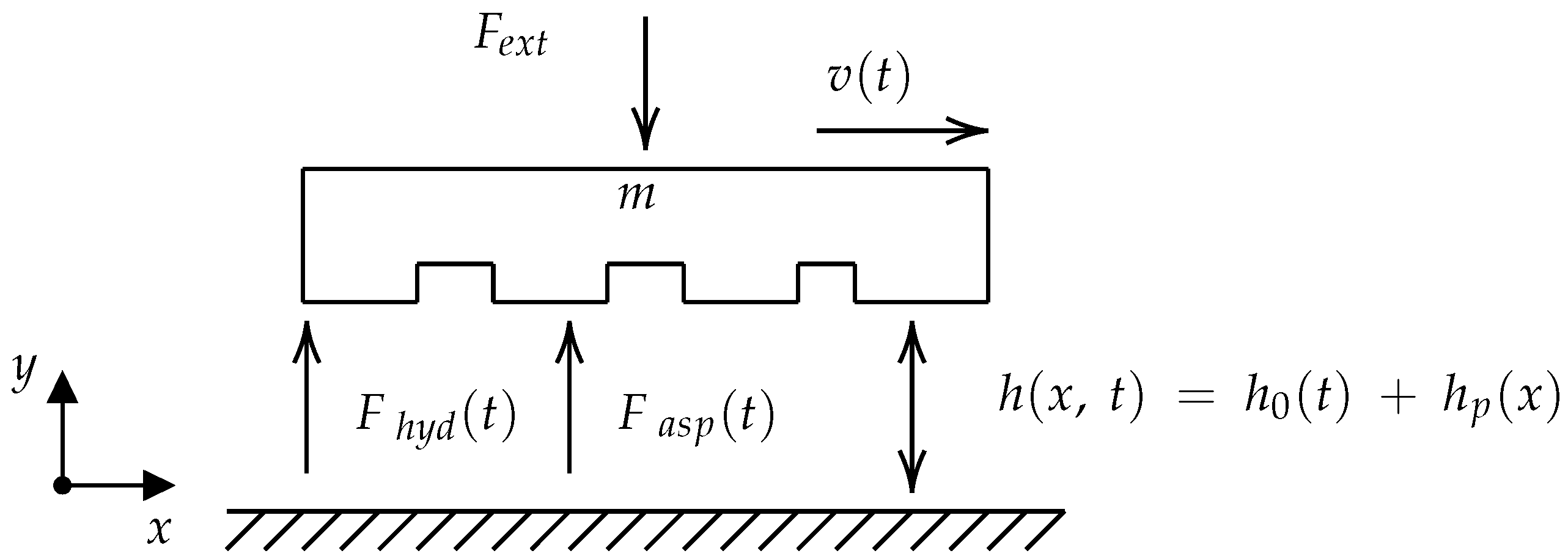
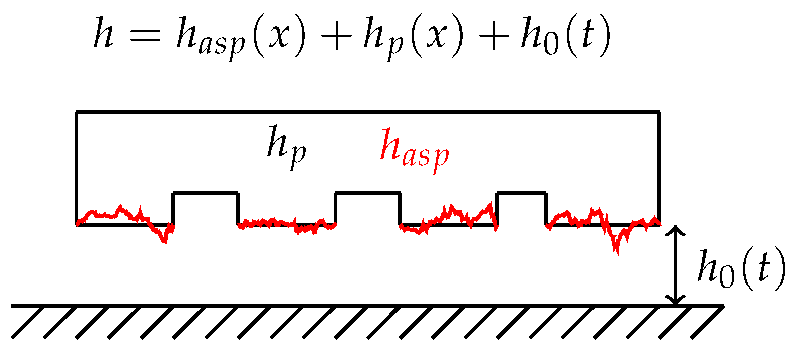
2. Non-Dimensional Model

The non-dimensional model developed in this work builds on the dimensional model constructed in [14], briefly outlined hereafter. Figure 1 depicts an overview of the lubricated contact geometry under investigation. The upper body is subjected to a constant external load ($F_{ext}$) alongside an oscillatory motion, induced by a sinusoidal sliding velocity ($v\left(t\right)$). The externally applied load is split into the hydrodynamic load ($F_{hyd}$) and the load contribution originating from asperity contact ($F_{asp}$), resulting in a mixed lubrication model.

As shown in previous work [14], the inertia of the bearing and the coupled system can be represented by an equivalent mass and is negligible in lightly loaded contacts with conformal geometry. In that study, we demonstrated that the inertial contribution scales with mass (m) and quadratically with sliding frequency (f). For typical systems considered, its influence on force equilibrium was estimated to be less than one promille and can therefore be safely neglected.

Neglecting inertia and tangential bearing displacements (Figure 1), the load balance is given by

$$F_{ext}=F_{hyd}+F_{asp}$$

(1)

in which, $F_{ext}$ is the external applied load per unit of length and $F_{asp}$, $F_{hyd}$ are respectively the asperity and hydrodynamic forces per unit of length. The asperity load $F_{asp}$ is modeled using the Greenwood-Williamson model [15],

$$\begin{array}{cc}\hfill F_{asp}& =E^{*}\eta {\beta }^{{\displaystyle \frac{1}{2}}}{\sigma }^{{\displaystyle \frac{3}{2}}}{A}_0{F}_{{\displaystyle \frac{3}{2}}}\left({\displaystyle \frac{h}{R_q}}\right)\hfill \\ \hfill & =A_{GW}{F}_{{\displaystyle \frac{3}{2}}}\left({\displaystyle \frac{h}{R_q}}\right)\mathrm{with}\hfill \end{array}$$

(2)

$$\begin{array}{cc}\hfill F_{{\displaystyle \frac{3}{2}}}(\Lambda )& ={\displaystyle \frac{1}{2\pi }}{\int }_{\Lambda }^{\infty }{\left(u-\Lambda \right)}^{{\displaystyle \frac{3}{2}}}\varphi \left(u\right)du\hfill \end{array}$$

(3)

$A_0$$\eta$, $\beta$ and $E^{*}$ denote respectively the real area, asperity density, mean curvature, and, the equivalent Young’s modulus of the surface. To ease the notation the surface parameters are lumped into $A_{GW}$. The surface height distribution is denoted as $\varphi \left(u\right)$.

The hydrodynamic contribution $F_{hyd}$ can be obtained from integrating the lubricants pressure profile over the contact domain:

$$F_{hyd}\left(t\right)={\int }_0^L{p}_h(x,t)dx$$

(4)

The fluid pressure $p\left(x\right)$ is determined by solving the transient Reynolds equation, subject to a set of Dirichlet Boundary conditions:

$${\displaystyle \frac{\partial }{\partial x}}\left({\displaystyle \frac{\rho h^3}{12\mu }}{\displaystyle \frac{\partial p}{\partial x}}\right)={\displaystyle \frac{U}{2}}{\displaystyle \frac{\partial \rho h}{\partial x}}+{\displaystyle \frac{\partial \rho h}{\partial t}}$$

(5)

$$\begin{array}{cc}\hfill p(x=0)& =0\hfill \\ \hfill p(x=L)& =0\hfill \end{array}$$

(6)

where h is the oil film thickness, U is the sliding velocity, and $\rho$ and $\mu$ are the lubricant density and dynamic viscosity, respectively. In this work, a Newtonian lubricant is considered with constant properties, limiting the scope to isothermal conditions.

The total friction force is determined by the combined contribution of the viscous shear of the fluid and the shear stress at the asperity contact:

$$\begin{array}{cc}\hfill F_f& =F_{f,hyd}+F_{f,asp}\hfill \\ \hfill & =B{\int }_0^L\left[\left(-{\displaystyle \frac{1}{2}}{\displaystyle \frac{\partial p}{\partial x}}h+{\displaystyle \frac{\mu v}{h}}\right)\right]dx+F_{asp}{\eta }_{bl}\hfill \end{array}$$

(7)

A constant boundary lubrication coefficient ${\eta }_{bl}$ is assumed, and B and L denote, respectively, the width and length of the contact.

The system of Equations (1)–(7) is solved for one cycle of reciprocating motion; this leads to a trajectory $h_0\left(t\right)$, $p(x,t)$. Hereafter using Equation (7), the friction force with time can be determined.

2.1. Non-Dimensional Formulation

The key of this work is to reformulate this transient mixed lubrication model above in a non-dimensional form, identifying non-dimensional groups or similarity parameters, allowing transparent identification and characterization of friction hysteresis behaviour. The normalization method in this work has been selected, as it is most convenient for the subsequent analysis of the specific problem under investigation. Note that other choices for normalization are possible.

The Equations (1)–(7) are non-dimensionalized by the substitution of the following normalized variables:

$$\begin{array}{c}\hfill \overline{x}={\displaystyle \frac{x}{\widehat{x}}};\overline{P}={\displaystyle \frac{P}{\widehat{P}}};\overline{t}={\displaystyle \frac{t}{\widehat{t}}};\overline{h}={\displaystyle \frac{h}{\widehat{h}}};\overline{\rho }={\displaystyle \frac{\rho }{\widehat{\rho }}};\\ \hfill \overline{\eta }={\displaystyle \frac{\eta }{\widehat{\eta }}};\overline{U}={\displaystyle \frac{U}{\widehat{U}}};\overline{F_n}={\displaystyle \frac{F_n}{\widehat{F_n}}};\overline{F_f}={\displaystyle \frac{F_f}{\widehat{F_f}}}\end{array}$$

(8)

The definition of the hatted values is further substantiated in the following paragraphs:

Film Thickness

Modelling the fluid film thickness as depicted in Figure 2, the bearing clearance is defined as:

$$\begin{array}{cc}\hfill h& =h_{asp}\left(x\right)+h_p\left(x\right)+h_0\left(t\right)\hfill \end{array}$$

(9)

$$\begin{array}{cc}\hfill h& =n{R}_q+h_p\left(x\right)+h_0\left(t\right)\hfill \end{array}$$

(10)

enabling the study of arbitrary profiles and textured surfaces. With $h_{asp}\left(x\right)$ and $h_p\left(x\right)$, respectively, the asperity height and the surface profile, $h_0\left(t\right)$ gives the time-dependent surface separation used to enforce a load balance. In this work, we opt to model the surface roughness in a statistical way, conforming to the Greenwood–Williamson contact model. In concreto, the deterministic asperity profile $h_{asp}\left(x\right)$ is replaced by a representative statistical mean, chosen to be proportional to the RMS surface roughness with proportionality constant n, i.e., $\widehat{h}=n{R}_q$. Varying the value of the normalization constant ‘n’ effectively scales the film thickness and alters the relative weight of contact and hydrodynamic contributions. While this does not affect the structure of the equations or dimensionless trends, it impacts interpretation when mapping back to dimensional quantities. The relationship between asperity height and root mean square (RMS) surface roughness has been a subject of interest in various studies [16,17]. However, in this work, we take n as unity for reasons of simplicity. Choosing the statistical asperity height as the reference for normalization, one obtains the non-dimensional Equation (11).

$$\begin{array}{cc}\hfill \overline{h}& =1+{\displaystyle \frac{h_p\left(x\right)}{n{R}_q}}+{\displaystyle \frac{h_0\left(t\right)}{n{R}_q}}\hfill \end{array}$$

(11)

Sliding Velocity

The oscillatory applied sliding velocity is given by:

$$U=U_0+U_{1}sin\left(2\pi ft\right)$$

(12)

Substitution of the normalized variables results in the following dimensionless expressions:

$$\begin{array}{c}\hfill \overline{U}={\displaystyle \frac{U_0}{U_1}}+sin\left(2\pi \overline{t}\right)\\ \hfill \overline{U}=U^{*}+sin\left(2\pi \overline{t}\right)\end{array}$$

(13)

With, $\widehat{t}={\displaystyle \frac{1}{f}}$, $\widehat{U}=U_1$, and $U^{*}={\displaystyle \frac{U_0}{U_1}}$. This normalization has been chosen to enable a straightforward description of the sliding velocity with and without offset ($U_0$). However, the sliding amplitude $U_1$ needs to be strictly positive to avoid singularities; hence, steady-state sliding cannot be simulated using this method.

Fluid Contribution

Substitution of the normalized variables into the Reynolds Equation (5), assuming an isoviscous and incompressible lubricant.

$$\begin{array}{cc}\hfill {\displaystyle \frac{\partial }{\partial \overline{x}}}\left({\displaystyle \frac{{(\overline{h}-1)}^3}{\overline{\mu }}}{\displaystyle \frac{\partial \overline{p}}{\partial \overline{x}}}\right)& =6H{e}^{*}\overline{U}{\displaystyle \frac{\partial (\overline{h}-1)}{\partial \overline{x}}}+12\sigma {\displaystyle \frac{\partial (\overline{h}-1)}{\partial \overline{t}}}\hfill \end{array}$$

(14)

with

$$\begin{array}{cc}\hfill AR\left(\mathrm{Aspect}\mathrm{Ratio}\right)& ={\displaystyle \frac{n{R}_q}{L}}\hfill \end{array}$$

(15)

$$\begin{array}{cc}\hfill H{e}^{*}\left(\mathrm{Bearing}\mathrm{Parameter}\right)& ={\displaystyle \frac{1}{A{R}^2}}{\displaystyle \frac{{\mu }_l{U}_1}{F_{ext}}}\hfill \end{array}$$

(16)

$$\begin{array}{cc}\hfill \sigma \left(\mathrm{Squeeze}\mathrm{Parameter}\right)& ={\displaystyle \frac{1}{A{R}^2}}{\displaystyle \frac{{\mu }_{l}Lf}{F_{ext}}}\hfill \end{array}$$

(17)

The non-dimensional viscosity can be given as follows:

$$\begin{array}{cc}\hfill \overline{\mu }& =1\hfill \end{array}$$

Cavitation is imposed into the system using Swift-Stiebel Conditions

$$\overline{p}=0\mathrm{when}\overline{p}\le 0$$

(18)

The non-dimensional hydrodynamic force becomes:

$${\overline{F}}_{n,hyd}={\int }_{\overline{x}=0}^{\overline{x}=1}\overline{p}d\overline{x}$$

(19)

The hydrodynamic force, obtained from integrating the pressure field, depends only on the ‘squeeze parameter’ ($\sigma$) and the ‘bearing parameter’ ($H{e}^{*}$).

Finally, the fluid frictional force in non-dimensional form is given as

$$\begin{array}{cc}\hfill {\overline{F}}_{f,hyd}& ={\displaystyle \frac{-1}{2}}AR\left({\int }_{\overline{x}=0}^{\overline{x}=1}{\displaystyle \frac{\partial \overline{p}}{\partial \overline{x}}}\overline{h}d\overline{x}+H{e}^{*}{\int }_{\overline{x}=0}^{\overline{x}=1}{\displaystyle \frac{\overline{\mu }\overline{U}}{\overline{h}}}d\overline{x}\right)\hfill \end{array}$$

(20)

Asperity Contribution

It is assumed that the maximum asperity forces occurs when the film thickness equals the combined root mean square surface roughness of both surfaces, indicating a normalized vertical separation of 1. This leads to the following non-dimensional expressions for asperity normal load and friction force:

$$\begin{array}{cc}\hfill F_{n,asp}& =\kappa F_{{\displaystyle \frac{3}{2}}}\left({\displaystyle \frac{\overline{h}}{m}}\right)\hfill \end{array}$$

(21)

$$\begin{array}{cc}\hfill \kappa \left(\mathrm{Contact}\mathrm{Parameter}\right)& ={\displaystyle \frac{A_{GW}{F}_{\frac{3}{2}}\left(m\right)}{F_{ext}}}\hfill \end{array}$$

(22)

here m is a placeholder number added to the equations to mitigate numerical problems during the calculations. The influence of the number m cancels out due to the inclusion in both the normal asperity force and in the contact parameter. In this paper the value of $m={\displaystyle \frac{3}{2}}$ is been chosen. The non-dimensional frictional force due to asperity contact is hence given as

$$\begin{array}{cc}\hfill {\overline{F}}_{f,asp}& =F_{\tau }{\overline{F}}_{n,asp}\hfill \end{array}$$

(23)

with $F_{\tau }=$ the friction coefficient.

Balance Equation

After substituting Equation (19) and Equation (21) in the balance equation and some manipulations, the non-dimensional force balance renders:

$$\begin{array}{c}\hfill {\overline{F}}_{n,hyd}+{\overline{F}}_{a,hyd}=1\end{array}$$

(24)

The total non-dimensional friction force is given:

$$\begin{array}{cc}\hfill {\overline{F}}_f& ={\displaystyle \frac{1}{F_{\tau }}}\left({\overline{F}}_{f,hyd}+{\overline{F}}_{f,asp}\right)\hfill \end{array}$$

(25)

2.2. Limitations of Model

As the main focus of our work is to map and gain insight into the friction hysteresis of low-loaded conformal contacts induced by reciprocating and oscillating motions, several simplifying assumptions are made in the present model. In this section, we summarize the simplifications. First, the lubricant is assumed to be Newtonian, and the flow is considered isothermal, thereby neglecting any thermal effects or shear-thinning behaviour. Neglecting shear-tinning behaviour limits the model to contacts with shear rates below approximately a threshold of ${10}^2{s}^{-1}$, a range within which many mineral-based lubricants exhibit near-Newtonian behaviour. Secondly, the rigid body motion of the bearing structure is assumed without inertia and constrained to the normal direction. Thirdly, contact is treated using the Greenwood-Williamson (GW) statistical model, which, while widely used, assumes a specific asperity distribution and does not capture all features of real asperity contact. It is to be noted that, due to the extensive utilization of the GW-contact theory in existing literature, its advantages, disadvantages, strengths, and weaknesses are well-documented [18,19,20,21,22]. Especially, in [22], an interesting overview and benchmark is given between GW-inspired models and numerically exact quantitative solutions of nominally flat contacts. It is to be noted that elastic coupling between surface deformation and the pressure field is not included. In addition, it is known that bearing-area models, such as GW, overestimate leakage by more than three decades [23]. Finally, the boundary lubrication is characterized by a constant coefficient, without accounting for its potential dependence on local contact conditions. These assumptions define the applicability of the model and should be considered when interpreting the results.

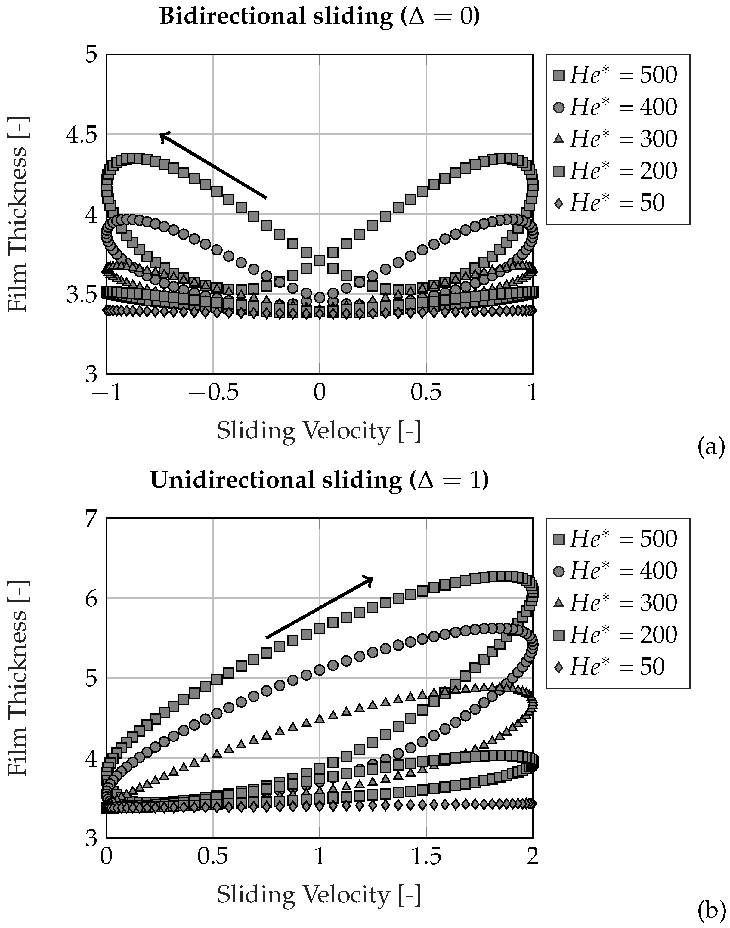
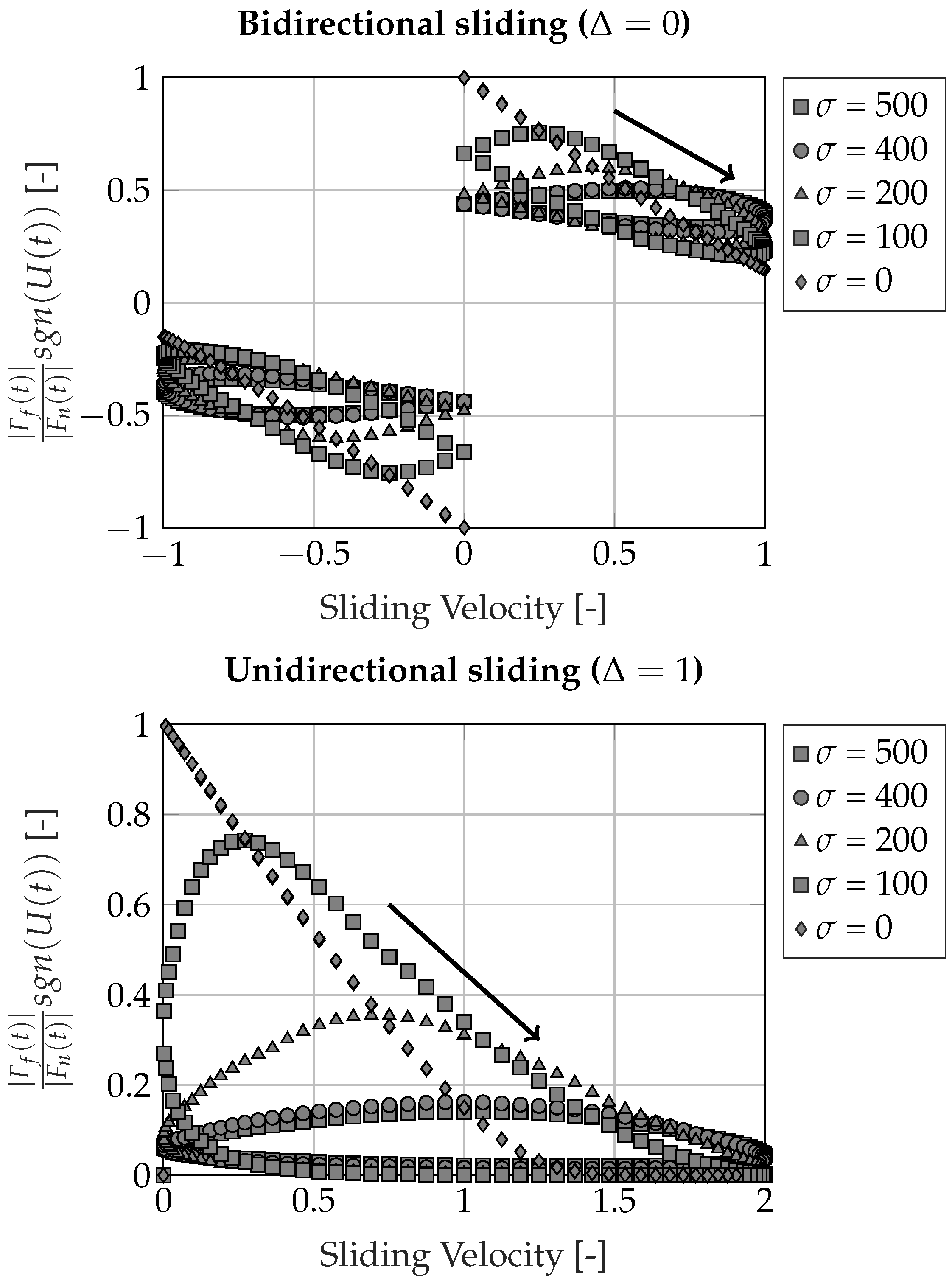
2.3. Discussion of Non-Dimensional Groups

Based on the non-dimensional formulation of the mixed friction model presented in the previous section, it becomes clear that friction hysteresis of rough conformal contacts can be described using six non-dimensional groups. Three non-dimensional groups are related to the lubricant flow, two are related to the asperity contact model, and one parameter characterizes the imposed velocity profile.

The proposed model can also be used to study the influence of hysteresis effects due to fluctuating normal loads. In this case, the system of six parameters is reduced to only four parameters ($U^{*},H{e}^{*},\sigma ,\omega$), simplifying the analysis.

In the following paragraph, these six parameters are summarized and discussed.

• The Velocity Ratio Parameter ($U^{*}={\displaystyle \frac{U_0}{U_1}}$) is a measure of the average sliding velocity of the system, around which the sinusoidal perturbation is applied. Using the absolute value of this parameter, three different sliding regimes are distinguished: (i) $U^{*}=0$, a pure sinusoidal sliding velocity is applied, (ii) $U^{*}\ge 1$, the sinusoidal motion can be seen as a perturbation around a mean value, and no motion reversal is occurring, (iii) $0<U^{*}<1$, motion reversal is still occurring; however, the sliding distance is not equal for both sides of the oscillation.
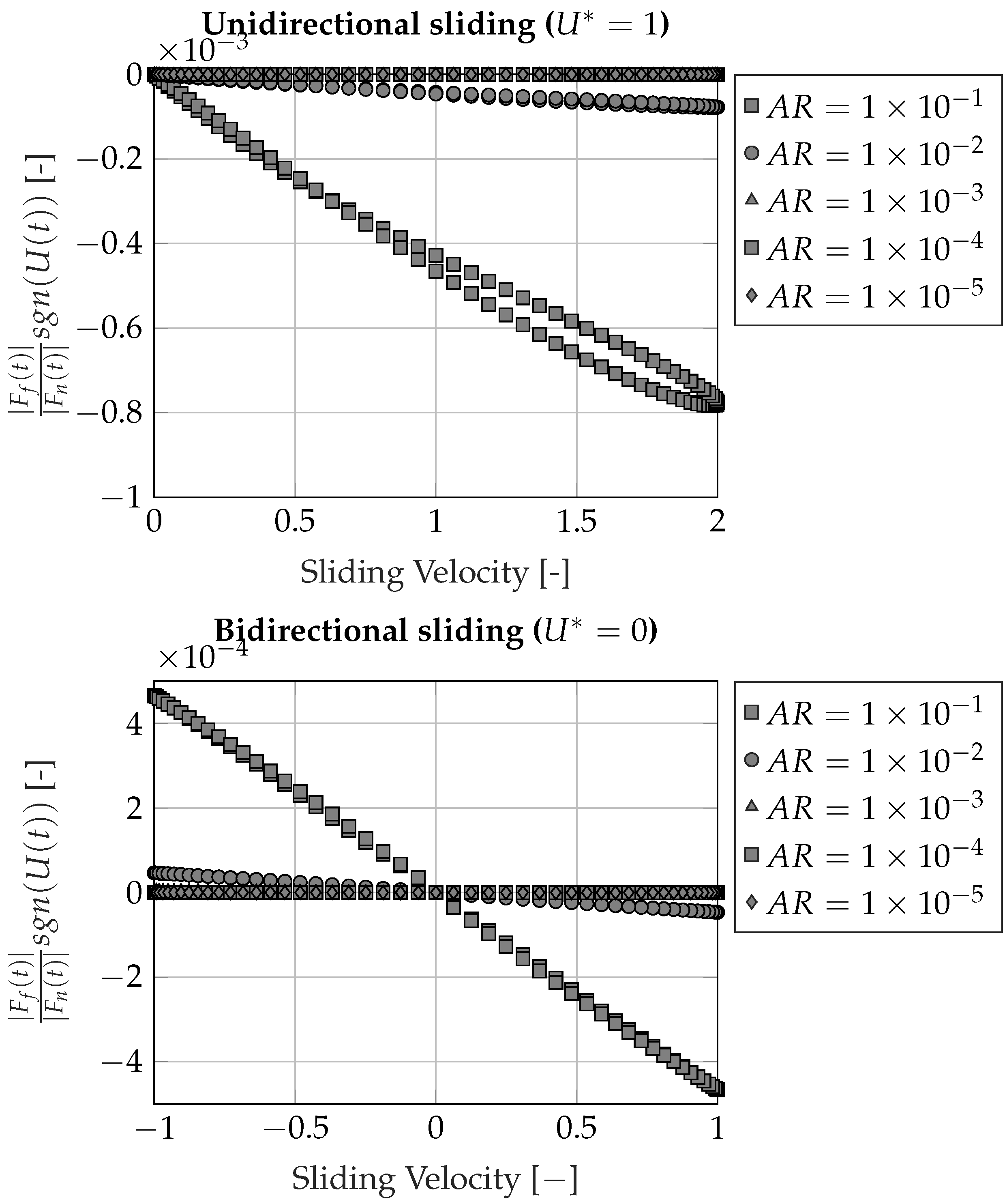
• The Aspect Ratio parameter ($AR={\displaystyle \frac{n{R}_q}{L}}$) is a measure of the clearance when subject to boundary lubrication relative to the length of the contact. Typical aspect ratios of non-conformal lightly loaded contacts are around 0.001 (Bearing dimensions in mm have typical roughness in m, and contacts in km scale have roughness in cm scale (i.e., roads)).
• The Bearing parameter ($H{e}^{*}={\displaystyle \frac{1}{A{R}^2}}{\displaystyle \frac{{\mu }_l{U}_1}{F_{ext}}}$) is equivalent to the Hersey number, rescaled with the aspect ratio, and expresses the relative importance of pressure to the viscosity contributions. The bearing parameter can be interpreted as the inverse of the Reynolds times the Euler number, indicating the magnitude of the pressure buildup w.r.t. the viscous lubricant flow. The $H{e}^{*}$ parameter should be strictly positive to ensure hydrodynamic pressure build-up.
• The Squeeze parameter ($\sigma ={\displaystyle \frac{1}{A{R}^2}}{\displaystyle \frac{{\mu }_{l}Lf}{F_{ext}}}$) is a measure for the squeeze contribution and is inversely proportional to the average pressure (external load divided by length) and proportional to the frequency. When the squeeze number equals zero, the contact reduces to steady-state operation.
• The Contact parameter ($\kappa ={\displaystyle \frac{A_{GW}{F}_{\frac{3}{2}}\left(\frac{3}{2}\right)}{F_{ext}}}$) determines the maximum load carried by the asperities when the film thickness equals the minimal possible clearance.
• The Friction parameter ($F_{\tau }={\eta }_{bl}{F}_{ext}$) is a measure of the maximum friction force that can occur due to asperity contact and is used to normalized the resulting friction force (i.e., combining asperity and hydrodynamic contributions) of the system. Hence, it can be used to determine in which friction regime the contact is operating.

Note that when the $\sigma$ and $H{e}^{*}$ parameters are compared, they differ in ${\displaystyle \frac{Lf}{U1}}$. Which can be understood as the ratio of the contact length L to the wavelength of the perturbation, i.e., ${\displaystyle \frac{U_1}{f}}$. As a ratio of lengths, this conceptually makes sense. Therefore, in Equation (14), one could consider substituting $\sigma$ with $H{e}^{*}$ times this velocity ratio in the second term.

Table 1. Dimensionless parameters, their definitions, and typical values.

Dimensionless Quantity	Symbol	Definition	Typical Value for Engineering Contacts
Velocity Ratio	$U^{*}$	${\displaystyle \frac{U_0}{U_1}}$	$0\le AR\le 10$
Aspect Ratio	$AR$	${\displaystyle \frac{n{R}_q}{L}}$	$\mathcal{O}\left({10}^{-3}\right)$
Bearing Parameter	$H{e}^{*}$	${\displaystyle \frac{1}{A{R}^2}}{\displaystyle \frac{{\mu }_l{U}_1}{F_{ext}}}$	$\mathcal{O}({10}^0$–${10}^3)$
Squeeze Parameter	$\sigma$	${\displaystyle \frac{1}{A{R}^2}}{\displaystyle \frac{{\mu }_{l}Lf}{F_{ext}}}$	$\mathcal{O}({10}^0$–${10}^3)$
Contact Parameter	$\kappa$	${\displaystyle \frac{A_{GW}{F}_{\frac{3}{2}}\left(\frac{3}{2}\right)}{F_{ext}}}$	$\mathcal{O}({10}^5$–${10}^7)$
Friction Parameter	$F_{\tau }$	${\eta }_{bl}{F}_{ext}$	$\mathcal{O}\left({10}^3\right)$

summarizes the non-dimensional quantities defined and used in this work. An indication of the typical value for a low-loaded metallic conformal engineering contact is presented.

3. Results and Discussion

By studying the impact of variations in specific non-dimensional groups, we aim to identify generalized self-similar tendencies. The investigations described below encompass systematic change of the parameters ($H{e}^{*},\sigma ,\omega ,\kappa ,...$), differentiating for each case between two scenario’s i.e., a unidirectional and biderectional motion.

The motion parameter $U^{*}$ is adjusted to examine two scenarios: first, an unidirectional one-way sliding that speeds up and slows down when $U^{*}$ is greater than one, and second, a bidirectional, reciprocating sliding when $U^{*}$ equals zero. A third situation, where the direction of motion changes at different sliding velocities and $U^{*}$ is between zero and one, is not discussed here to keep things simple.

A hysteresis loop can be split into two main parts, an upper branch and a lower branch, depending on the acceleration and deceleration of the slider accordingly.

In this publication, the simulation cases are run for a parabolic slider, as described in references [14,24,25,26], and the parabolic slider is visualized in Figure 3. The tabulated input parameters (

Table 2. Operational Conditions for the Non-Dimensional Sliding Simulations.

Parameter	Value
$AR$	0.001
$H{e}^{*}$	500
$\sigma$	250
$\kappa$	1,120,000
$F_{\tau }$	6300
$U^{*}$	1
$\Delta x$	$256\times 1$
$\Delta t$	0.01

) are determined based on the values used in previously mentioned papers and used for the non-dimensional parameters unless otherwise noted.

3.1. Parameter Study

Variation with Contact Parameter-$\kappa$

The contact parameter $\kappa$ was systematically varied within the range of 1000 to 500,000 for both unidirectional and bidirectional motion, as illustrated in Figure 4. Two distinct phenomena were observed in both cases.

When $\kappa$ is high, the non-dimensional friction force nearly reaches one as velocity approaches zero, indicating that asperities primarily support the load. $\kappa$ reflects the stiffness of the contact, with a higher $\kappa$ resulting in a higher asperity normal load at the same gap separation. As velocity increases, friction decreases, suggesting more of the applied load is carried by hydrodynamic lubrication. Conversely, for small values of $\kappa$, the maximum value of the friction force is significantly lower, implying that most of the load is supported by the hydrodynamic film, and the importance of squeeze damping is more pronounced.

Note that for $\kappa >50,000$, under the simulated conditions, the effect of $\kappa$ becomes less pronounced. Hence, the influence of $\kappa$ on the morphology of the friction hysteresis loop is limited. Thus, in subsequent studies, a typical contact parameter, depending on the material of the contact pair, can be adopted (e.g., metallic rough surfaces around ${10}^5$–${10}^6$, plastic surfaces around ${10}^3$–${10}^4$, etc.), limiting the amount of non-dimensional numbers that need to be varied.

Variation with Aspect Ratio Parameter-$AR$

The Aspect Ratio parameter, denoted as $AR$, was systematically varied over five orders of magnitude, ranging from ${10}^{-1}$ to ${10}^{-5}$. The results, presented in Figure 5, indicate that under the given simulation conditions the total friction force remains largely unaffected by changes in $AR$.

To understand this behaviour, we refer to the definition of $AR$ in Section 2.1 and its role in the hydrodynamic friction force, as expressed in Equation (20). According to Equation (20), a decrease in $AR$ leads to a reduction in the fluid friction force while the asperity friction force is unaffected. In addition, the $AR$ does not influence the normal load balance (Equation (24)). Hence, the chance in $AR$, while keeping the other non-dimensional parameters constant, relates to a chance in lubrication regime.

This effect is further illustrated in Figure 6, where only the fluid friction force is visualized. The results show that for increasing $AR$, the fluid friction force becomes smaller and smaller. Under the current simulation conditions, where the contact operates within the mixed lubrication regime, the contribution of fluid friction to the total force is already limited. This reduction in fluid friction force (${10}^{-3}$) is negligible in comparison with the asperity friction (${10}^0$), resulting in a nearly unchanged total friction force. Consequently, while $AR$ affects the relative contributions of fluid and asperity friction, its overall impact on the friction hysteresis loops remains minimal.

Variation with Bearing Parameter-$H{e}^{*}$

Figure 7 illustrates the variations in the friction hysteresis loop corresponding to different values of the bearing parameter. Three discernible trends come to light: (i) the friction hysteresis loop demonstrates an increase in magnitude, where the magnitude refers to the vertical span of the loop, representing the difference between the maximum and minimum friction forces occurring within a cycle; (ii) the mean friction force over the entire oscillation is decreasing with increasing $H{e}^{*}$; and (iii) the morphology, or shape, of the friction hysteresis loop undergoes a transformation from a narrow loop to a more bulky shape with increasing $H{e}^{*}$. The loop area increases with increasing bearing parameter. An increase in $H{e}^{*}$ means higher velocity fluctuations, i.e., higher acceleration and deceleration, and thus higher squeeze contributions, which in turn explains the bigger loops.

To clarify these observed behaviours, the film thickness is presented in Figure 8. Here, it is evident that an increase in $H{e}^{*}$ is accompanied by an increase in maximum film thickness. In addition, the film thickness loop area is also increasing with an increasing bearing parameter. Additionally, Figure 8b highlights that, even at zero velocity, a discernible film thickness persists with increasing $H{e}^{*}$, contributing to a friction value lower than the boundary friction coefficient. This phenomenon is consistent with the observations presented in Figure 7b.

Variation with Squeeze Number-$\sigma$

Figure 9 provides a comprehensive visualization of the impact of the squeeze number, denoted as $\sigma$, on friction hysteresis. Friction hysteresis loops were generated across a spectrum of $\sigma$ values, ranging from 0 to 500. In accordance with prior research, it is noted that the most pronounced friction loops occur in the mixed friction regime. For this analysis, specific values of $H{e}^{*}$ were chosen to operate within this regime. The intricate interplay of the $H{e}^{*}$ and $\sigma$ parameters is deferred to further elaboration in Section 3.2.

When the squeeze number approaches zero, the curve converges to the steady-state curve, as illustrated in Figure 9. As the $\sigma$ parameter increases, a departure from the steady-state curve becomes evident, accompanied by an observable increase in loop size. Additionally, it is observed that an increase in the squeeze number corresponds to a decrease in the peak friction coefficient of friction.

Three key observations emerge:

First, an increase in the variable $\sigma$ leads to a larger loop size for both unidirectional ($\Delta =1$) and bidirectional ($1l$) sliding. As $\sigma$ increases, the contribution of hydrodynamic load to the overall friction also rises for a given velocity. This results in a transition from friction dominated by asperities to one dominated by hydrodynamic effects. Consequently, there is a more noticeable difference in friction between the accelerating and decelerating phases of the oscillation.

Second, a higher $\sigma$ also results in reduced friction at the point where the direction reverses. This is due to a higher squeeze number, which generates greater hydrodynamic pressure for the same sliding velocity. More of the applied load is then supported by the fluid film rather than the asperities, leading to a reduction in friction force.

Third, the orientation of the hysteresis loops remains aligned with the steady-state curve, but the loops rotate counterclockwise as $\sigma$ increases. This indicates that at lower velocities, the friction force occurring during the hysteresis loop is lower than what would be predicted by a steady-state model. The increase in film thickness with a higher squeeze number suggests that a larger portion of the external load is supported by the fluid film rather than the asperities.

Figure 10 further shows that for very large squeeze numbers a dimensionless film thickness of about 3.5 is attained when the velocity is zero for a bearing number of 500. The value of the minimal film thickness at zero velocity depends both on the bearing and squeeze number, indicating that the external load is fully supported by the fluid film, which originates from the squeeze generation. However, as the contacts transition into the mixed regime (as depicted in the middle column of Figure 9), high $\sigma$ values prompt deviations from the Stribeck curve, accompanied by a counter-clockwise rotation of the loop axis.

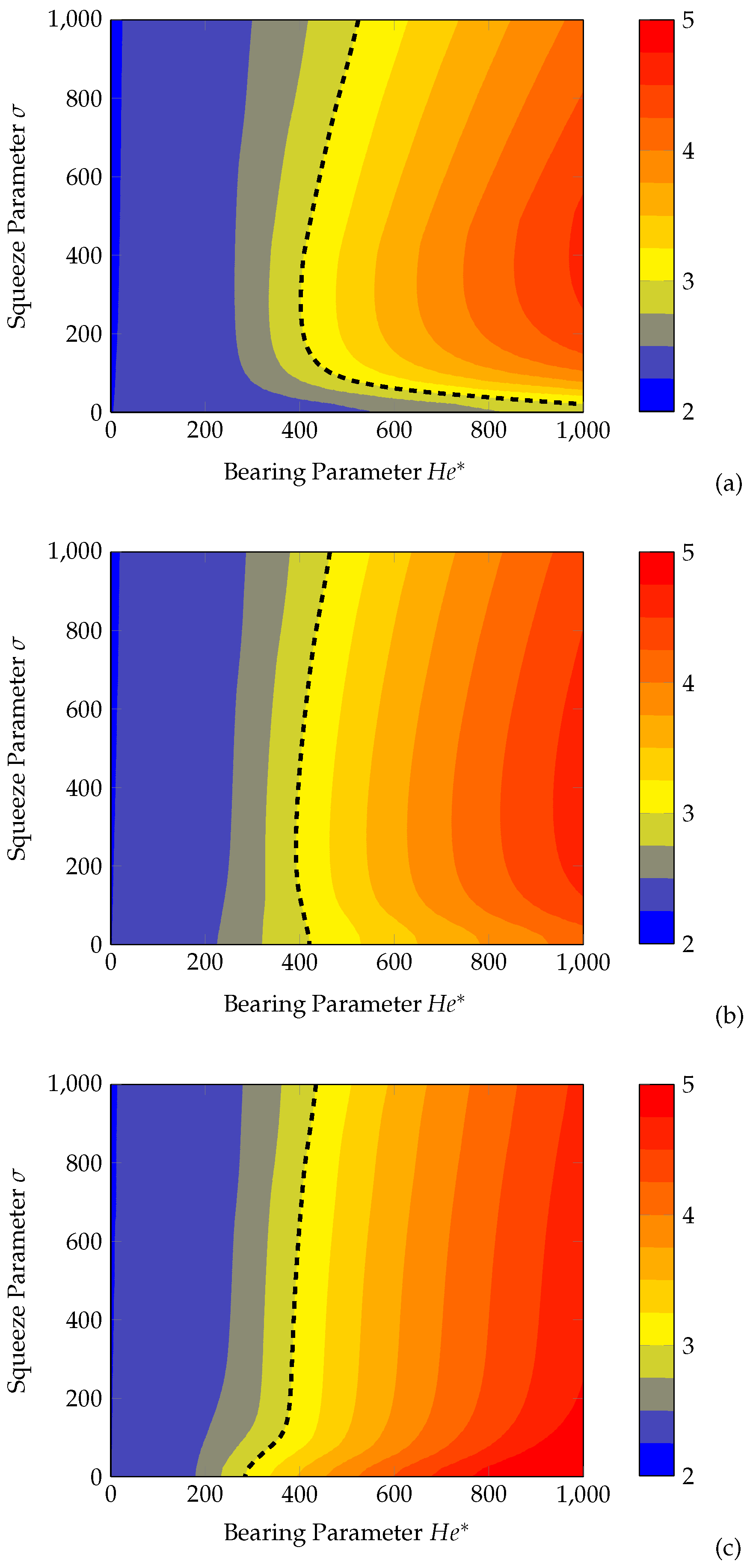
3.2. Parameter Analysis

From the preceding sections, it is clear that only the bearing and squeeze parameters emerge as the most significant determinants shaping the observed frictional behaviour. In light of these findings, we aim to make parametric maps as function of those dimensionless parameters, indicating under which conditions the lubrication regime is occurring and the influence of the lubrication regime on the friction hysteresis loop.

Selecting the specific values for the bearing and squeeze parameters is crucial for defining the morphology of the friction hysteresis loop, which in turn depends on the instantaneous lubrication regime. Figure 11 will clearly show how these non-dimensional parameters affect friction hysteresis. Understanding these effects is key to explaining the hysteresis loop’s morphology and behaviour.

To facilitate this analysis, the instantaneous lubrication regime should be determined. Therefore, the instantaneous non-dimensional height, denoted as $\overline{h}$, is divided by a scaling factor $m={\displaystyle \frac{3}{2}}$, as indicated in Equation (21). In the context of this study, a pragmatic assumption is made: when ${\displaystyle \frac{\overline{h}}{1.5}}\ge 3$, the contact is assumed to operate in full film lubrication. Conversely, when ${\displaystyle \frac{\overline{h}}{1.5}}\le 1.5$, the contact is considered to be in a boundary lubrication regime. For values falling in-between this range, the contact is classified as operating in the mixed lubrication regime.

This approach enables a classification of lubrication regimes based on the non-dimensional height, providing a straightforward means of associating different segments of the friction hysteresis loop—such as acceleration and deceleration phases—with their corresponding lubrication conditions. In addition, the ’dominant’ lubrication regime is identified as the one in which the oscillating contact operates for the majority of the oscillation cycle. By analysing these three regimes simultaneously, an understanding of the intricate lubrication dynamics is presented.

While the classification based upon film thickness provides a convenient metric, it can be argued that there exist other methods to determine the lubrication regime and the severity of a certain lubrication regime (e.g., asperity-hydrodynamic force balance, area of contact, etc.). However, the classification in this work was used as a tool to investigate if and how the dominant lubrication regime differs between the accelerating and decelerating phases of the friction hysteresis loop. A more refined classification (with more granularity) could be developed in future work.

In Figure 11, the visualization of the non-dimensional height, and thus the lubrication regime, is presented for varying bearing ($H{e}^{*}$) and squeeze ($\sigma$) parameters. The graph shows the lubrication regime for the entire loop and for the accelerating and deceleration phase. A dashed line is used to indicate the transition line from mixed lubrication to full film lubrication.

From Figure 11 a pattern emerges in which the role of $H{e}^{*}$ and $\sigma$ determines the dominant lubrication regime for each segment of the hysteresis loop w.r.t. the dominant lubrication regime of the entire oscillation. The dominant lubrication regime is determined by the amount of time the contact resides in each lubrication regime. The dominant lubrication regime appears quasi-independent of the squeeze number and is limitedly influenced by variations in the bearing parameter. By overlapping the three figures of Figure 11, five unique regions can be determined, each associated with a distinct friction hysteresis loop profile, as indicated in Figure 12.

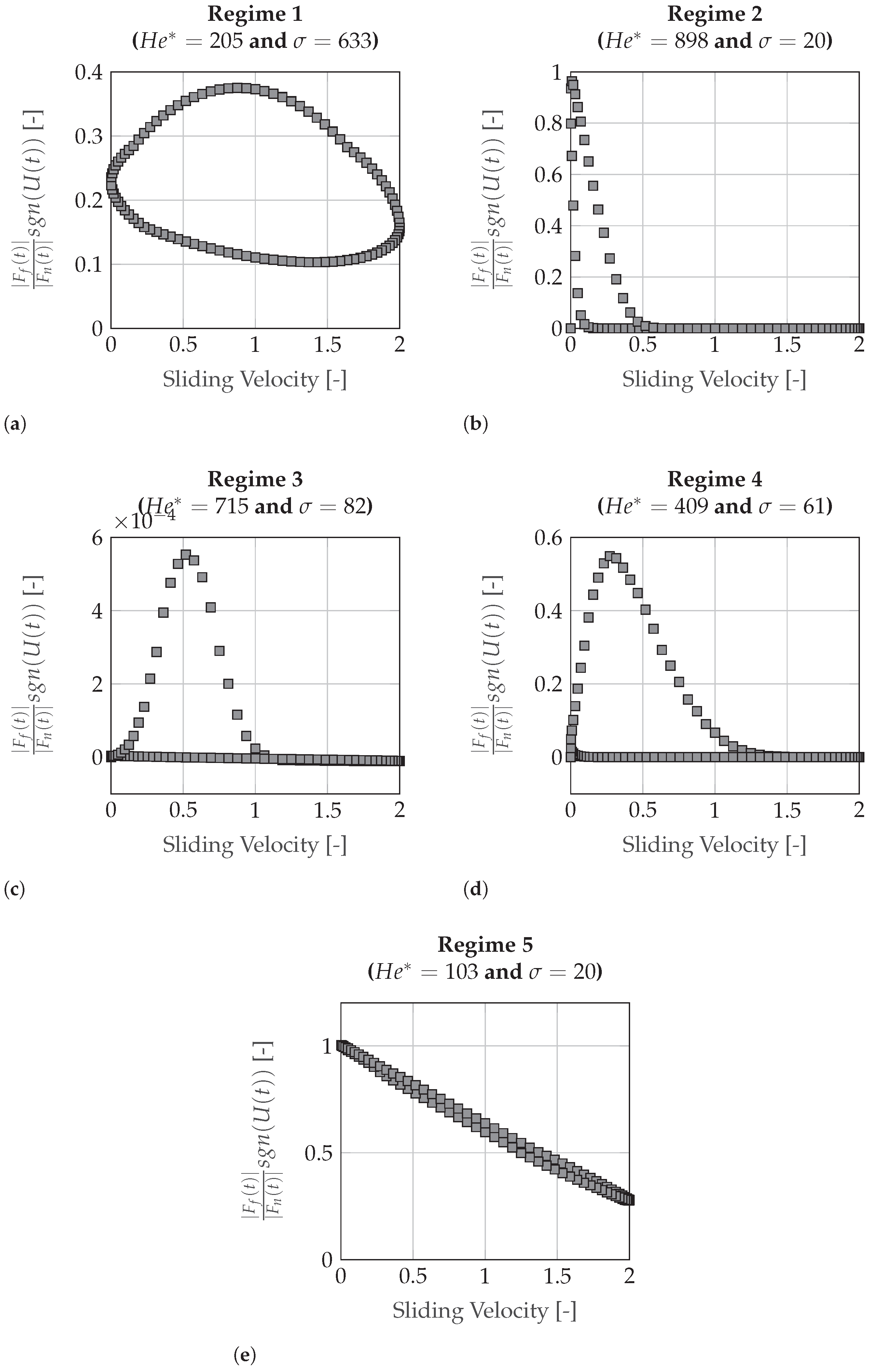
• Regime 1: Characterized by a quasi-circular friction hysteresis loop, where both acceleration and deceleration phases are in the mixed friction regime. A rather high squeeze value is present, leading to a quasi-circular friction loop and an overall lower friction value as compared with Regime 5, contributing to the observed loop.
• Regime 2: Represents a scenario where the upper branch is in the mixed lubrication regime, while the lower branch operates in the full film regime. The hysteresis loop exhibits symmetry and closely follows the Stribeck curve.
• Regime 3: Distinguished by extremely low friction values and a relatively small hysteresis loop. Both phases of the loop operate in the full friction regime, facilitated by elevated bearing and squeeze numbers.
• Regime 4: Occupies a transitional position where the upper branch is in the mixed regime, while the lower branch is entirely in the full regime. This results in highly asymmetric friction loops with substantial differences between both phases.
• Regime 5: In this regime, the contact operates in both acceleration and deceleration phases within the mixed friction regime. Additionally, this regime is subjected to relatively low values of the squeeze number. The outcome is narrow, quasi-straight hysteresis loops with a notably large coefficient of friction.

4. Conclusions

In this paper, a non-dimensional mixed lubrication model is developed, encompassing a transient Reynolds equation and a statistical contact equation, along with a load balance equation. Featuring a set of non-dimensional groups that facilitate the investigation of friction hysteresis in rough and lubricated contacts. The investigation encompasses the impact of parameters such as contact, friction, aspect ratio, bearing, squeeze, and the interplay between them on the friction hysteresis loops. Through numerical evaluations of this model under varying non-dimensional parameters, a systematic study of friction hysteresis is conducted, leading to meaningful conclusions.

Parameter Influence

• Contact and Friction Parameters:

  -

  The contact and friction parameters exhibit limited influence on friction hysteresis loops, with variations within a 10% threshold.

  -

  The friction parameter, $\mu$, serves as a scaling factor without a pronounced effect on the loops, reaffirming its role in boundary lubrication coefficient incorporation.

• Aspect Ratio Parameter:

  -

  The aspect ratio parameter, $AR$, demonstrates negligible influence on friction hysteresis loops, especially in non-conformal, lightly loaded scenarios. The Aspect Ratio (AR) primarily affects the fluid friction force but has minimal impact on the total friction force, which is the sum of both fluid and asperity friction forces.

• Bearing, Squeeze, and Contact Parameters:

  -

  Bearing, squeeze, and contact parameters emerge as significant determinants, defining lubrication regimes for different loop phases.

  -

  Graphical analysis identifies five unique regions based on bearing and squeeze parameters, each associated with characteristic friction hysteresis loop profiles.

Identified Friction hysteresis Regimes

• Regime 1: Bulky friction hysteresis loop with both phases in the mixed friction regime, influenced by a high squeeze value.
• Regime 2: Symmetric loop with up-going phase in the mixed regime and down-going phase in the full film regime.
• Regime 3: Extremely low friction values with both phases operating in the full friction regime, characterized by high bearing and squeeze numbers.
• Regime 4: Transitional regime with asymmetric friction loops, where the up-going phase is in the mixed regime and the down-going phase is entirely in the full regime.
• Regime 5: Narrow, quasi-straight hysteresis loops with a large friction value, where both phases operate in the mixed friction regime with low squeeze values.

These more advanced modelling techniques include the incorporation of thermal effects, non-Newtonian lubricant behaviour, and more sophisticated asperity models that account for adhesion, anisotropy and real surface topographies. Additionally, the integration of coupling between contact and fluid film is identified as a promising direction for enhancing model accuracy and relevance to real-world applications. Besides more advanced modelling, future research could be carried out on interactions between the non-dimensional groups that may lead to complex behaviours not fully captured in the current study. While the current study focuses primarily on single-parameter variations, future work can include a systematic parametric sweep to explore coupled effects and potential nonlinear interactions.

In conclusion, this study sheds light on friction hysteresis dynamics and emphasizing the pivotal roles of bearing, squeeze, and contact parameters. The identified regimes provide a valuable framework for associating specific lubrication conditions with characteristic frictional behaviours. These insights contribute to a comprehensive understanding of the diverse operational scenarios influencing friction hysteresis, facilitating informed design and optimization strategies in tribological applications. Future research may further delve into the complexities of parameter interactions, more advanced modelling techniques and their implications for more nuanced system design.

References

1. Armstrong-Hélouvry, B.; Dupont, P.; De Wit, C.C. A survey of models, analysis tools and compensation methods for the control of machines with friction. Automatica 1994, 30, 1083–1138. [Google Scholar] [CrossRef]
2. Olsson, H. Control Systems with Friction. Ph.D. Thesis, Department of Automatic Control, New Jersey Institute of Technology, Newark, NJ, USA, 1996. [Google Scholar]
3. Lampaert, V.; Al-Bender, F.; Swevers, J. Experimental Characterization of Dry Friction at Low Velocities on a Developed Tribometer Setup for Macroscopic Measurements. Tribol. Lett. 2004, 16, 95–105. [Google Scholar] [CrossRef]
4. van Geffen, V. A Study of Friction Models and Friction Compensation; Technical Report for TU Eindhoven: Eindhoven, The Netherlands, 2009. [Google Scholar]
5. De Moerlooze, K. Contributions to the Characterisation of Friction and Wear: Theoretical Modelling and Experimental Validation. Ph.D. Thesis, KU Leuven Faculteit Ingenieurswetenschappen, Leuven, Belgium, 2010. [Google Scholar]
6. Rabinowicz, E. The Intrinsic Variables affecting the Stick-Slip Process. Proc. Phys. Soc. 1958, 71, 668–675. [Google Scholar] [CrossRef]
7. Hess, D.P.; Soom, A. Friction at a Lubricated Line Contact Operating at Oscillating Sliding Velocities. J. Tribol. 1990, 112, 147–152. [Google Scholar] [CrossRef]
8. Lu, X.; Khonsari, M.M. An Experimental Study of Grease-Lubricated Journal Bearings Undergoing Oscillatory Motion. J. Tribol. Trans. Asme 2007, 129. [Google Scholar] [CrossRef]
9. Lu, X.; Khonsari, M.M. An Experimental Study of Oil-Lubricated Journal Bearings Undergoing Oscillatory Motion. J. Tribol. 2008, 130, 021702. [Google Scholar] [CrossRef]
10. Zhai, X.; Needham, G.; Chang, L. On the Mechanism of Multi-Valued Friction in Unsteady Sliding Line Contacts Operating in the Regime of Mixed-Film Lubrication. J. Tribol. 1997, 119, 149–155. [Google Scholar] [CrossRef]
11. Sojoudi, H.; Khonsari, M.M. On the Modeling of Quasi-Steady and Unsteady Dynamic Friction in Sliding Lubricated Line Contact. J. Tribol. 2009, 132, 012101. [Google Scholar] [CrossRef]
12. Harnoy, A.; Friedland, B. Dynamic Friction Model of Lubricated Surfaces for Precise Motion Control. Tribol. Trans. 1994, 37, 608–614. [Google Scholar] [CrossRef]
13. Sampson, J.B.; Morgan, F.; Reed, D.W.; Muskat, M. Studies in Lubrication: XII. Friction Behavior During the Slip Portion of the Stick-Slip Process. J. Appl. Phys. 1943, 14, 689–700. [Google Scholar] [CrossRef]
14. Driesen, K.; Castagne, S.; Lauwers, B.; Fauconnier, D. On the Numerical Modeling of Friction Hysteresis of Conformal Rough Contacts. Lubricants 2023, 11, 326. [Google Scholar] [CrossRef]
15. Greenwood, J.A.; Williamson, J.P. Contact of nominally flat surfaces. Proc. R. Soc. London Ser. A. Math. Phys. Sci. 1966, 295, 300–319. [Google Scholar] [CrossRef]
16. Chang, L.; Jeng, Y.R. Effects of Negative Skewness of Surface Roughness on the Contact and Lubrication of Nominally Flat Metallic Surfaces. Proc. Inst. Mech. Eng. Part J. Eng. Tribol. 2012. [Google Scholar] [CrossRef]
17. Zhou, W.; Zhao, D.; Tang, J.; Yi, J. A Comparative Study on Asperity Peak Modeling Methods. Chin. J. Mech. Eng. 2021. [Google Scholar] [CrossRef]
18. Maaboudallah, F.; Najah, M.; Atalla, N. A Review on the Contact Mechanics Modeling of Rough Surfaces in the Elastic Regime: Fundamentals, Theories, and Numerical Implementations. In Tribology of Machine Elements; Pintaude, G., Cousseau, T., Rudawska, A., Eds.; IntechOpen: Rijeka, Croatia, 2022; Chapter 3. [Google Scholar] [CrossRef]
19. Taylor, R.I. Rough Surface Contact Modelling—A Review. Lubricants 2022, 10, 98. [Google Scholar] [CrossRef]
20. Ciavarella, M.; Delfine, V.; Demelio, G. A “re-vitalized” Greenwood and Williamson model of elastic contact between fractal surfaces. J. Mech. Phys. Solids 2006, 54, 2569–2591. [Google Scholar] [CrossRef]
21. Ciavarella, M.; Greenwood, J.; Paggi, M. Inclusion of “interaction” in the Greenwood and Williamson contact theory. Wear 2008, 265, 729–734. [Google Scholar] [CrossRef]
22. Müser, M.H.; Dapp, W.B.; Bugnicourt, R.; Sainsot, P.; Lesaffre, N.; Lubrecht, T.A.; Persson, B.N.J.; Harris, K.; Bennett, A.; Schulze, K.; et al. Meeting the Contact-Mechanics Challenge. Tribol. Lett. 2017, 65, 118. [Google Scholar] [CrossRef]
23. Dapp, W.B.; Lücke, A.; Persson, B.N.J.; Müser, M.H. Self-Affine Elastic Contacts: Percolation and Leakage. Phys. Rev. Lett. 2012, 108, 244301. [Google Scholar] [CrossRef]
24. Sahlin, F.; Almqvist, A.; Larsson, R.; Glavatskih, S. A cavitation algorithm for arbitrary lubricant compressibility. Tribol. Int. 2007, 40, 1294–1300. [Google Scholar] [CrossRef]
25. Bertocchi, L.; Dini, D.; Giacopini, M.; Fowell, M.T.; Baldini, A. Fluid film lubrication in the presence of cavitation: A mass-conserving two-dimensional formulation for compressible, piezoviscous and non-Newtonian fluids. Tribol. Int. 2013, 67, 61–71. [Google Scholar] [CrossRef]
26. Profito, F.; Giacopini, M.; Zachariadis, D.; Dini, D. A General Finite Volume Method for the Solution of the Reynolds Lubrication Equation with a Mass-Conserving Cavitation Model. Tribol. Lett. 2015, 60, 18. [Google Scholar] [CrossRef]
Figure 1. Schematic overview of the model.
Lubricants 13 00248 g001
Figure 2. Schematic overview of the film thickness model, roughness is indicated in red.
Lubricants 13 00248 g002
Figure 3. Non-Dimensional surface profile of the slider bearing.
Lubricants 13 00248 g003
Figure 4. Non-Dimensional Friction Force Variation with κ , an arrow indicates the accelerating phase of the oscillation. Further dimensional parameters: A R = 0.001 , H e * = 500 , σ = 250 , M = 0.3 , U * = 1 .
Lubricants 13 00248 g004
Figure 5. Non-Dimensional Friction Force Variation with A R , an arrow indicates the accelerating phase of the oscillation. Further dimensional parameters: H e * = 250 , σ = 250 , κ = 1,120,000, M = 0.3 , U * = 1 .
Lubricants 13 00248 g005
Figure 6. Non-Dimensional Fluid Friction Force Variation with A R . Further dimensional parameters: H e * = 250 , σ = 250 , κ = 1,120,000, M = 0.3 .
Lubricants 13 00248 g006
Figure 7. Non-Dimensional Friction Force Variation with H e * , an arrow indicates the accelerating phase of the oscillation. Further dimensional parameters: A R = 0.001 , σ = 250 , κ = 1,120,000, M = 0.3 , U * = 1 .
Lubricants 13 00248 g007
Figure 8. Non-Dimensional Fluid Film Thickness Variation with H e * , an arrow indicates the accelerating phase of the oscillation. Further dimensional parameters: A R = 0.001 , σ = 250 , κ = 1,120,000, M = 0.3 , U * = 1 .
Lubricants 13 00248 g008
Figure 9. Non-Dimensional Friction Force Variation with σ , an arrow indicates the accelerating phase of the oscillation. Further dimensional parameters: A R = 0.001 , H e * = 500 , κ = 1,120,000, M = 0.3 , U * = 1 .
Lubricants 13 00248 g009
Figure 10. Non-Dimensional Fluid Film Thickness Variation with σ , an arrow indicates the accelerating phase of the oscillation. Further dimensional parameters: A R = 0.001 , H e * = 500 , κ = 1,120,000, M = 0.3 , U * = 1 .
Lubricants 13 00248 g010
Figure 11. Non-Dimensional height of unidirectional sliding with varying squeeze and bearing number (a) accelerating phase, (b) entire loop, and (c) decelerating phases. The transition line between mixed and full film is indicated with a dashed line.
Lubricants 13 00248 g011
Figure 12. Five typical observed Friction Hysteresis Loops (ae).
Lubricants 13 00248 g012