Development of a Non-Uniform Heat Source Model for Accurate Prediction of Wheel Tread Temperature on Long Downhill Ramps

Abstract

Accurately simulating the thermal behavior of wheel–brake shoe friction on long downhill ramps is challenging due to the complexity of modeling appropriate heat source models. This study investigates heat generation during the frictional braking process of freight train wheels and brake shoes under long-slope conditions. Four heat source models—constant, modified Gaussian, sinusoidal, and parabolic distributions—were developed based on energy conservation principles and validated through experimental data. A thermomechanical coupled finite element model was established, incorporating a moving heat source to analyze the effects of different models on wheel tread temperature distribution and its evolution over time. The results show that all four models effectively simulate frictional heat generation, with computed temperatures, deviating by only 6.0–8.2% from experimental measurements, confirming their accuracy and reliability. Among the models, the modified Gaussian distribution heat source, with its significantly higher peak local heat flux (2.82 times that of the constant model) and rapid attenuation, offers the most precise simulation of the non-uniform temperature distribution in the contact region. This leads to a 40% increase in the temperature gradient variation rate and effectively reproduces the “hot spot” effect. The new non-uniform heat source model accurately captures local temperature dynamics and predicts frictional heat transfer and thermal damage trends. The modified Gaussian distribution model outperforms others in simulating local temperature peaks, offering support for optimizing braking system models and improving thermal damage prediction. Future research will refine this model by incorporating factors like material wear, environmental conditions, and dynamic contact characteristics.

1. Introduction

Freight trains inevitably undergo braking during operation, and the braking system is a crucial safeguard for operational safety. Currently, tread braking remains one of the commonly used braking methods for freight trains due to its advantages, including simple installation, low cost, and the ability to grind the wheel tread profile [1]. With the increase in train speed and service frequency, the thermal load on railway freight wagon wheels has been steadily increasing, making wheel tread thermal fatigue damage a critical issue in heavy-haul railway transportation.

During long downhill ramps, freight trains rely on the continuous frictional contact between wheel treads and brake shoes to convert and dissipate kinetic and gravitational potential energy into heat. Extended braking under these conditions significantly increases thermal load, posing severe challenges to braking performance and operational safety. Due to sustained frictional contact between the wheel and the brake shoe, heat is generated and transferred between the two components. The higher the freight train speed and axle load, the greater the kinetic energy, leading to a rapid rise in temperature in both the wheel and brake shoe. Under tread braking, frequent frictional contact causes the wheel tread temperature to regularly exceed 400 °C [2], and under complex operating conditions such as gradient braking, it may even exceed 600 °C [3,4].

Elevated temperatures cause thermal softening in the materials of both the wheel and brake shoe [5], reducing their yield strength. Additionally, due to the temperature-dependent nature of wheel materials, high temperatures may also induce phase transformations in the metallic microstructure. Vo et al. [6] reported that a martensitic white layer forms when rail steel reaches 720 °C. Al-Juboori et al. [7] further proposed that the formation of the martensitic white layer occurs at the austenitic transformation temperature, which, for deformed microstructures (ferrite-pearlite), is typically around 700 °C [8]. Martensite is regarded as a major contributor to wheel tread damage. Overall, the high thermal load generated by tread braking can lead to various forms of wheel tread damage, including hot spots [9], thermal cracks [10], corrugation [11], shelling [12], and spalling [13], all of which severely compromise train operational safety. The root cause of thermal fatigue damage to the wheel tread is the extreme thermal load and the complex contact behavior experienced by the wheel tread. Throughout the entire tread braking cycle, the interaction between the wheel and the brake shoe exhibits thermal elastic instability (TEI) [14], resulting in significant inhomogeneity in the thermal load on the wheel tread.

In the calculation of frictional heating between the wheel and the brake shoe, significant research has been undertaken. The calculation of frictional heating between the wheel and brake shoe typically employs experimental methods [15], analytical methods [16], and numerical methods [17,18,19]. However, the experimental approach, which directly measures the wheel tread temperature, is relatively complex and costly. Analytical and numerical methods, as effective tools for predicting surface temperatures, have been widely adopted. Analytical methods often rely on simplified assumptions and idealized models (such as linear material assumptions and the neglect of certain effects), which may not reflect actual conditions, thereby diminishing the accuracy and reliability of the results. Wasilewski [20] reviewed specific numerical modeling methods for railway tread braking frictional heating and highlighted that modeling the frictional heating of friction components during the design phase can reduce experimental costs. The article recommends further development of existing models to account for the interaction between numerical models, operational conditions, and the friction coefficient. As a numerical method, the finite element method (FEM) is widely used in the study of frictional temperature rise between the wheel and brake shoe due to its simplicity, cost-effectiveness, and efficiency.

Regarding the modeling dimensions for finite element analysis of wheel–brake shoe frictional heating, many scholars have conducted research, categorizing models into one-dimensional [21,22], two-dimensional (2D) [23,24,25,26,27,28], and three-dimensional (3D) [29,30] frictional temperature rise models. Kuciej et al. [31] compared the temperature fields obtained from a three-dimensional wheel–brake shoe frictional heating finite element model with those from a two-dimensional axial wheel–brake shoe frictional heating finite element model. Their findings suggest that, considering both computational accuracy and efficiency, the two-dimensional wheel–brake shoe finite element model is a more ideal choice.

Based on the calculation methods for frictional heating between the wheel and the brake shoe, two approaches can be identified: one that creates a frictional contact pair between the wheel and the brake shoe, and the other that applies thermal boundary conditions. Due to the low computational efficiency of establishing frictional contact pairs between friction components, this approach is rarely used. Instead, applying thermal boundary conditions has been widely adopted as it simplifies the model and offers higher computational efficiency while maintaining relatively accurate computational precision.

When applying thermal boundary conditions for heat analysis, there are two methods for constructing and applying the heat source. For the first approach, to simplify the computation, the thermal boundary condition method typically adopts a uniform heat source, assuming that the heat flux is evenly distributed along the circumferential direction of the wheel tread, with the heat source covering the entire tread and remaining stationary. Owing to the high-speed rotational friction between the wheel and the brake shoe, the time for one full revolution of the wheel during braking is very short. Therefore, the assumption of a uniformly acting heat flux over the entire wheel tread is reasonably justified. For this method, some researchers have adopted this approach to conduct modeling studies on tread braking [32,33,34,35,36]. Based on this method, Zhang et al. [37] investigated the temporal evolution of the temperature field on the wheel tread under long downhill conditions and analyzed the influence of braking thermal loads on the propagation of thermal cracks in the wheel tread. Yuan et al. [38], using the brake disc as a case study, conducted a modified investigation of this method and proposed a new heat source calculation approach suitable for more accurate prediction of frictional temperature rise in brake discs.

The other approach involves applying a moving heat source load on the wheel tread to simulate the repeated contact and separation between the wheel and the brake shoe. Compared to the former method, this approach more accurately reflects real-world conditions. Based on this moving heat source method, Milošević [2] used the finite element method to conduct numerical simulations, integrating analytical modeling with numerical techniques to investigate the thermal effects of the braking system. A three-dimensional wheel–brake shoe friction finite element model was established, with thermal boundary conditions applied to calculate the temperature fields of the wheel and brake shoe. However, this method assumes a uniformly distributed moving heat source over the wheel–brake shoe contact interface, which differs from the actual frictional heat distribution in wheel–brake contact. Lian et al. [39] employed the Goldak heat source model [40] to calculate the frictional temperature rise between the wheel and rail. This method was used to evaluate the thermal impact on the rail after repeated wheel passes. A comparison between the moving heat source method and a three-dimensional thermomechanical coupling approach revealed only minor temperature differences. Yuan et al. [41,42] focused on the frictional heat generation between wheel and rail, and pointed out that the Goldak heat source model [40] is not suitable for such contact scenarios. Based on the principle of energy conversion, they proposed a moving heat source method that accounts for the actual shape of the contact patch between wheel and rail and verified its accuracy. Zhang et al. [43] compared the frictional temperature rise under different creepages using two methods: direct calculation based on a moving heat source derived from Hertzian contact and a fully coupled thermomechanical finite element model. Their study established a finite element model for frictional heating between wheel and rail, showing that the temperature difference between the two methods was within 5%. Based on the above references, these findings suggest that the development of accurate heat source models still requires further investigation.

In summary, most existing moving heat source modeling methods focus on the frictional contact between the wheel and rail, whereas significant differences exist between wheel–rail and wheel–brake shoe frictional contact characteristics. In the current literature, studies on the construction of frictional heat sources between the wheel and brake shoe are scarce. Moreover, in actual braking processes, the frictional contact state between the wheel and brake shoe exhibits pronounced spatiotemporal non-uniformity, influenced by factors such as contact pressure distribution, local sliding velocity, and material properties. The resulting frictional heat source is non-uniform and varies dynamically over time and space. Temperature distributions calculated using the uniform heat source method often deviate significantly from real-world conditions, failing to capture local temperature gradients and “hotspot” effects [9] on the wheel tread. However, the accurate prediction of wheel tread temperature fields is critical for evaluating braking performance and assessing thermal damage risks. Therefore, how to construct a more accurate frictional heat source model for the wheel–brake shoe interface remains an open research question that needs to be addressed.

Based on the moving heat source method, which can more realistically simulate the frictional heat generation between the wheel and brake shoe, this study proposes a non-uniform heat source model to better capture the actual thermal behavior. Based on the principle of energy equivalence, this study proposes an improved frictional contact heat source model for the wheel and brake shoe, constructing and validating four heat source forms: constant, modified Gaussian, sinusoidal, and parabolic distributions. The new model systematically considers the rotational frictional contact behavior between the wheel and brake shoe, allowing for a more accurate description of the true shape of the friction contact area and its heat flux distribution characteristics. To simulate tread braking under long downhill slope conditions, a two-dimensional finite element model of the wheel was developed. By establishing three-dimensional and two-dimensional indirectly coupled thermomechanical finite element models and integrating them with the moving heat source method, the temperature evolution of the wheel tread was simulated and analyzed. The validity of the model was verified through comparison with previously published references and experimental data. The results show that the modified Gaussian distribution heat source captures the local temperature rise characteristics more accurately, significantly enhances the rate of change in temperature gradient, and more realistically reproduces the transient “hotspot” effects in the friction contact area.

The novel friction heat source modeling method proposed in this study provides new theoretical support for the prediction of thermal damage in the braking systems of freight trains on long gradients and offers valuable reference for the braking optimization design of rail transportation and heavy-load transport systems. Future research will further optimize the heat source model, considering friction material wear [44], environmental variables [45], and dynamic contact characteristics [46] to enhance the model’s applicability under complex conditions and expand its engineering application value.

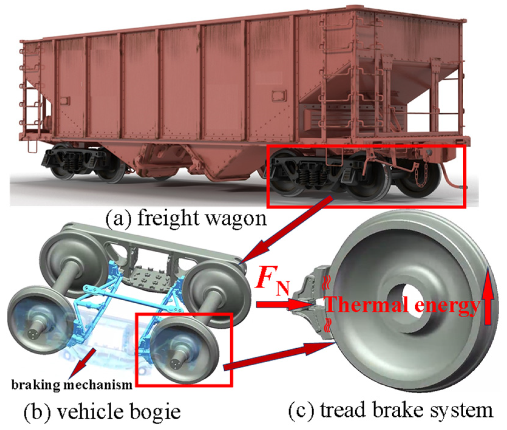
This study investigates the tread braking process of freight trains on long and steep slopes where brake shoes press against the rotating wheels and braking energy is generated at the frictional contact surface between the wheel and the brake shoe. Figure 1 illustrates the research methodology and technical workflow of this study.

First, an equivalent model of the tread braking system is established based on the actual geometric structure of the freight train’s wheel and brake shoe. To more accurately study the equivalent heat source model applicable to the tread braking of wheels on long downhill ramps, both 3D and 2D wheel–brake shoe friction indirectly coupled thermomechanical finite element models are established. The 3D model, with its more accurate results, is mainly used to calculate the temperature distribution on the wheel tread, while the 2D model, known for its higher computational efficiency, is used to simulate the temperature evolution of the wheel tread over time. During the tread braking process, the thermal boundary conditions between the wheel, brake shoe, and surrounding environment are considered, including thermal input boundary conditions (heat flux) and thermal output boundary conditions (heat convection and radiation). Corresponding thermal analysis boundary conditions are applied to the wheel and brake shoe to simulate the real friction process of the wheel–brake shoe interface. To accurately simulate this frictional braking behavior, several equivalent wheel–brake shoe friction contact heat sources are proposed, including a constant heat source, a modified Gaussian distribution heat source, a sine distribution heat source, and a parabolic distribution heat source. After constructing the heat sources, the moving heat source method is applied, with heat sources rotating around the wheel tread. The load application method is based on the ANSYS 17.0 table load method, constructing “heat flux load tables” and “convective heat transfer load tables”. The heat source models are then validated by theoretical analysis and experimental comparison. Finally, the temperature distribution on the wheel tread and the temperature history in both circumferential and radial directions are compared for the four heat source methods, and the results are compared with experimental data to verify the validity of the model.

2. Dynamic Heat Source Models

In this section, heat source models for the wheel–brake shoe frictional contact are established. First, a numerical heat transfer theory model is established. Second, it is assumed that the heat source at the contact between the wheel and brake shoe is uniformly distributed along the axial direction. Based on the principle of energy conservation, the frictional heat source between the wheel and brake shoe is equivalently represented by a constant heat source, a modified Gaussian distribution heat source, a sinusoidal distribution heat source, and a parabolic distribution heat source.

2.1. Numerical Modeling of Frictional Heat Transfer in Railway Wheel Braking Systems

During tread braking processes, frictional heat is generated at the wheel–brake shoe interface as the rotating wheel interacts with the brake shoe. The resultant thermal energy rapidly propagates into both the wheel and brake shoe components, inducing substantial alterations in their respective temperature fields. This complex heat transfer phenomenon is governed by partial differential equations of heat conduction. In accordance with the energy conservation principle, the temporal rate of energy change within a control volume equals the net heat input rate through boundaries plus the volumetric heat generation rate. For a unit control volume, the governing heat conduction equation is expressed as:

$$\rho c{\displaystyle \frac{\partial T}{\partial t}}=-\nabla ·\mathbf{q}+E$$

(1)

In the equation, ρ represents the density (kg/m³), c represents the specific heat capacity (J/(kg·°C)), T indicates the temperature value (°C), t represents time (s), ∂T/∂t corresponds to the rate of change of temperature with respect to time (°C/s), q represents the heat flux vector (W/m²), −∇ · q quantifies the divergence of heat flux (W/m³), and E is the rate of generation of the heat source per unit volume, (W/m³).

In accordance with Fourier’s law of heat conduction, the heat flux vector exhibits direct proportionality to the negative temperature gradient, formulated as the constitutive equation:

$$\mathbf{q}=-k\nabla T$$

(2)

In the equation, k denotes the thermal conductivity (W/(m·°C)), and ∇T represents the temperature gradient (°C/m).

The constitutive relation defined by Fourier’s law is systematically incorporated into the governing heat conduction equation, yielding the following refined formulation:

$$\rho c{\displaystyle \frac{\partial T}{\partial t}}=k{\nabla }^{2}T+E$$

(3)

In the equation, ∇²T denotes the Laplacian operator acting on the temperature field (°C/m²).

Within the framework of the Cartesian coordinate system, the spatial operators are explicitly defined as:

$${\nabla }^{2}T={\displaystyle \frac{{\partial }^{2}T}{\partial x^2}}+{\displaystyle \frac{{\partial }^{2}T}{\partial y^2}}+{\displaystyle \frac{{\partial }^{2}T}{\partial z^2}}$$

(4)

In the equation, x, y, and z are defined as the orthogonal coordinates in the Cartesian coordinate system.

The governing heat conduction equation in Cartesian coordinates is expressed in its expanded form as:

$$\rho c{\displaystyle \frac{\partial T}{\partial t}}=k{\displaystyle \frac{{\partial }^{2}T}{\partial x^2}}+k{\displaystyle \frac{{\partial }^{2}T}{\partial y^2}}+k{\displaystyle \frac{{\partial }^{2}T}{\partial z^2}}+E$$

(5)

For the wheel finite element model, during the element discretization process, quadrilateral elements are preferentially adopted for 2D simulations to ensure computational accuracy, while hexahedral elements are systematically employed for 3D configurations to maintain grid quality and solution convergence.

For the wheel finite element model, the polynomial interpolation of the nodal temperature is:

$$T={\displaystyle \sum _{i=1}^m{N}_i\left(x,y,z\right)}{T}_i=\left[N\right]\left\{T\right\}$$

(6)

In the equation, $\left\{N\right\}$ represents the shape function of the element, and $\left\{T\right\}$ is the vector of nodal temperatures of the element, where the number of nodes is m and the number of elements is n.

Solving the heat conduction control equation is equivalent to solving the optimization problem of finding the extremum of Equations (7) and (8).

$$\begin{array}{l}Z(T)=-{\displaystyle {\iint }_{S_{\mathrm{r}}}q}TdS+{\displaystyle \frac{1}{2}}{\displaystyle {\iiint }_v\left[\lambda {\left(\frac{\partial T}{\partial x}\right)}^2+\lambda {\left(\frac{\partial T}{\partial y}\right)}^2+\lambda {\left(\frac{\partial T}{\partial z}\right)}^2+2\rho c\left(\frac{\partial T}{\partial t}\right)T\right]dV}\\ \hspace{1em}\hspace{1em}\hspace{1em}+{\displaystyle \frac{1}{2}}{\displaystyle {\iint }_{S\mathrm{e}-S_{\mathrm{r}}}\left[h{\left(T-T_{\mathrm{A}}\right)}^2+\epsilon \sigma {\left(T^4-T_{\mathrm{A}}^4\right)}^2\right]}dS\end{array}$$

(7)

$$Z={\displaystyle \sum _{j=1}^n{Z}^e}$$

(8)

In the equation, S_r represents the frictional contact surface between the wheel and the brake shoe, S_e represents the external surface of the wheel and brake shoe, S_e–S_r refers to the surfaces other than the contact area, h represents the convective heat transfer coefficient (W/(m²·°C)), T_A is the ambient temperature (°C), ε is the emissivity, σ is the Stefan–Boltzmann constant (W/(m²·°C⁴)), Z^e is the function for each element, and Z is the function for the entire finite element model.

Let ${\displaystyle \frac{\partial Z^e}{\partial T_i}}=0$, and the total equation is given as follows:

$$\left[C\right]\left[{\displaystyle \frac{\partial T}{\partial t}}\right]+(\left[K_{\lambda }\right]+\left[K_H\right]+\left[K_E\right])\left[T\right]=\left[Q\right]$$

(9)

In the equation, [K_λ] is the total thermal conductivity matrix, [K_H] is the total thermal convection matrix, [K_E] is the total thermal radiation matrix, [C] is the specific heat matrix, and [Q] is the heat flux matrix. Each matrix represents the contribution of the corresponding thermal transfer mechanism to the overall thermal behavior. [T] and [∂T/∂t] represent the column vector of the node temperatures and their time derivatives, respectively.

2.2. Constant Distributed Heat Source Model

During tread braking operations, the brake shoe maintains continuous contact with the rotating wheel through the application of normal force. The frictional interaction between these components converts mechanical work into thermal energy at the wheel–brake shoe interface. This energy generation mechanism originates from the shared frictional work contributions of both contacting bodies. Governed by thermal conduction principles and surface tribological characteristics, the resultant frictional power undergoes partitioned distribution between the wheel and brake shoe.

Applying the frictional power distribution methodology, the instantaneous power allocation into each component is quantified as:

$$W_{\mathrm{w}/\mathrm{b}}={\eta }_{\mathrm{w}/\mathrm{b}}{\mu }_{\mathrm{wb}}{F}_{\mathrm{nwb}}{V}_{\mathrm{s}}$$

(10)

In the equation, η_w/b represents the heat partitioning factor for the wheel/brake shoe part, μ_wb is the friction coefficient between the wheel and the brake shoe, F_nwb is the normal contact force between the wheel and the brake shoe (N), and V_s is the relative velocity between the wheel and the brake shoe (m/s).

According to reference [47], the heat partitioning factor is determined by Equations (11)–(14). The calculation method for the heat partitioning factor between the wheel and brake shoe is as follows:

$${\beta }_{\mathrm{w}/\mathrm{b}}=\sqrt{k_{\mathrm{w}/\mathrm{b}}·{\rho }_{\mathrm{w}/\mathrm{b}}·c_{\mathrm{w}/\mathrm{b}}}$$

(11)

$${\eta }_{\mathrm{w}/\mathrm{b}}={\displaystyle \frac{{\beta }_{\mathrm{w}/\mathrm{b}}·A_{\mathrm{w}/\mathrm{b}}}{{\beta }_{\mathrm{b}/\mathrm{w}}·A_{\mathrm{b}/\mathrm{w}}+{\beta }_{\mathrm{w}/\mathrm{b}}·A_{\mathrm{w}/\mathrm{b}}}}$$

(12)

$$A_{\mathrm{w}}=2·\mathsf{\pi }·R_{\mathrm{w}}·\delta$$

(13)

$$A_{\mathrm{b}}=L_{\mathrm{b}}·\delta$$

(14)

In the equation, β_w/b is the thermal diffusivity of the wheel/brake shoe (m²/s), k_w/b is the thermal conductivity of the wheel/brake shoe (W/(m·°C)), ρ_w/b is the density of the wheel/brake shoe (kg/m³), c_w/b is the specific heat capacity of the wheel/brake shoe (J/(kg·°C)), A_w is the heat flux action area on the wheel (m²), A_b is the heat flux action area on the brake shoe (m²), L_b is the length of the brake shoe (m), δ is the effective contact width between the wheel and the brake shoe (m), and R_w is the radius of the wheel (m).

Assuming the frictional energy generated during braking is uniformly distributed across the wheel–brake shoe tribopair, a steady-state uniform volumetric heat source model is established. When using the moving heat source method, the resultant constant heat flux imposed on the wheel (Q_w-const) is formulated based on the frictional power dissipation and nominal contact area. Figure 2 illustrates the spatial power density distribution profile of the constant distributed heat source model.

$$Q_{\mathrm{w}\text{-}\mathrm{const}}=Q_0={\displaystyle \frac{W_{\mathrm{w}}}{S_{\mathrm{moving}}}}$$

(15)

$$S_{\mathrm{moving}}=A_{\mathrm{b}}=L_{\mathrm{b}}·\delta$$

(16)

In the equation, S_moving represents the contact area between the wheel and the brake shoe (m²).

Given the inherent geometric mismatch in wheel–brake shoe contact configurations, where the circumferential contact area of the wheel tread significantly surpasses that of the brake shoe, the minimal contact area (corresponding to the brake shoe) is systematically adopted for thermal characterization. The brake shoe interface is geometrically defined with length L_b (mm) and critical contact width b = 0.085 m. In any given moment of the wheel–brake shoe contact, the thermal excitation is constrained within the z = 0 interfacial plane, occupying the spatial domain 0 ≤ x ≤ L_b (circumferential direction) and 0 ≤ y ≤ b (axial direction). Under these geometrically constrained conditions, the heat flux function q_constant-w (x,y,z) is mathematically formulated as a spatially bounded distribution, as shown in Equation (17).

$$q_{\mathrm{constant}\text{-}\mathrm{w}}\left(x,y,z\right)=\left\{\begin{array}{cc}{Q}_{\mathrm{w}\text{-}\mathrm{const}}& 0\le x\le L_{\mathrm{b}},0\le y\le b\\ 0& \mathrm{otherwise}\end{array}\right.$$

(17)

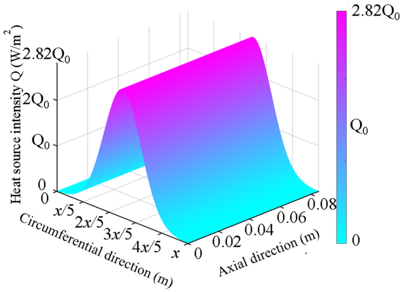
2.3. Modified Gaussian Distributed Heat Source Model

The advantage of the Gaussian heat source lies in its ability to accurately model the concentrated heat region while ensuring rapid heat dissipation with increasing distance. In heat conduction problems, the Gaussian heat source is usually described using a three-dimensional Gaussian distribution to represent the spatial distribution of the heat source, where the heat variation along a specific direction exhibits symmetry. Based on the Gaussian heat source, we established a modified Gaussian distribution heat source model for the interaction between the wheel and the brake shoe.

Assuming a local coordinate system at the brake shoe contact interface, where the normal of the contact surface lies in the x-y plane and the normal direction perpendicular to this plane is defined as the z-axis, this study assumes that the contact pressure between the wheel and the brake shoe varies only along the x-y plane while remaining uniformly distributed along the z-direction (wheel’s axial direction). In the x-y plane, the heat source follows a Gaussian distribution, which can be expressed as:

$$q_{\mathrm{gaussian}\text{-}\mathrm{w}}\left(x\right)=Q_{\mathrm{w}\text{-}\mathrm{const}}·e^{-C{\left(x-{\displaystyle \frac{W}{2}}\right)}^2}$$

(18)

In the equation, W is the length of one period.

Its area over a period [0, W] is given by:

$$A_{\mathrm{original}}={\displaystyle {\int }_0^W{q}_{\mathrm{gaussian}\text{-}\mathrm{w}}\left(x\right)}dx=Q_{\mathrm{w}\text{-}\mathrm{const}}·{\displaystyle \frac{\sqrt{\mathsf{\pi }}}{\sqrt{C}}}·\mathrm{erf}\left({\displaystyle \frac{W\sqrt{C}}{2}}\right)$$

(19)

In the equation, ${\displaystyle \frac{\sqrt{\mathsf{\pi }}}{\sqrt{C}}}$ is the normalization factor for the Gaussian distribution (representing the full area in the absence of truncation). $\mathrm{erf}\left({\displaystyle \frac{W\sqrt{C}}{2}}\right)$ is the error function, which denotes the proportion of the Gaussian distribution contained within the finite interval [0, W].

Based on the principle of power conservation, in order to ensure that the area of the Gaussian heat source equals the target area A_target, the amplitude of the Gaussian heat source needs to be adjusted. The adjusted amplitude is denoted as Q_adjusted.

$$q_{\mathrm{gaussian}\text{-}\mathrm{w}\text{-}\mathrm{adjusted}}\left(x\right)=Q_{\mathrm{adjusted}}·e^{-C{\left(x-{\displaystyle \frac{W}{2}}\right)}^2}$$

(20)

$$A_{\mathrm{target}}=Q_{\mathrm{w}\text{-}\mathrm{const}}·T$$

(21)

The adjusted Gaussian heat source area over a period [0, W] is:

$$A_{\mathrm{adjusted}}={\displaystyle {\int }_0^W{q}_{\mathrm{gaussian}\text{-}\mathrm{w}\text{-}\mathrm{adjusted}}\left(x\right)}dx=Q_{\mathrm{adjusted}}·{\displaystyle \frac{\sqrt{\mathsf{\pi }}}{\sqrt{C}}}·\mathrm{erf}\left({\displaystyle \frac{W\sqrt{C}}{2}}\right)$$

(22)

In order to ensure that the adjusted Gaussian heat source area equals the constant heat source area, the following condition must be satisfied.

$$A_{\mathrm{adjusted}}=A_{\mathrm{target}}$$

(23)

The magnitude of the adjusted amplitude can be obtained.

$$Q_{\mathrm{adjusted}}·{\displaystyle \frac{\sqrt{\mathsf{\pi }}}{\sqrt{C}}}·\mathrm{erf}\left({\displaystyle \frac{W\sqrt{C}}{2}}\right)=Q_{\mathrm{w}\text{-}\mathrm{const}}·W$$

(24)

$$Q_{\mathrm{adjusted}}={\displaystyle \frac{Q_{\mathrm{w}\text{-}\mathrm{const}}·W·\sqrt{C}}{\sqrt{\mathsf{\pi }}·\mathrm{erf}\left(\frac{W\sqrt{C}}{2}\right)}}$$

(25)

Therefore, the constructed modified Gaussian distributed heat source model is:

$$q_{\mathrm{gaussian}\text{-}\mathrm{w}\text{-}\mathrm{adjusted}}\left(x\right)={\displaystyle \frac{Q_{\mathrm{w}\text{-}\mathrm{const}}·W·\sqrt{C}}{\sqrt{\mathsf{\pi }}·\mathrm{erf}\left(\frac{W\sqrt{C}}{2}\right)}}·e^{-C{\left(x-{\displaystyle \frac{W}{2}}\right)}^2}$$

(26)

In the equation, x is the coordinate variable, C is the parameter that controls the width of the Gaussian distribution. In the calculations of this study, C is set to 0.01, which corresponds to the Gaussian distribution type heat source form at this point. Figure 3 shows the contour plot of the modified Gaussian distribution heat source model. From the contour plot, it can be observed that the peak magnitude of the Gaussian distribution heat source is 2.82 times that of the constant heat source.

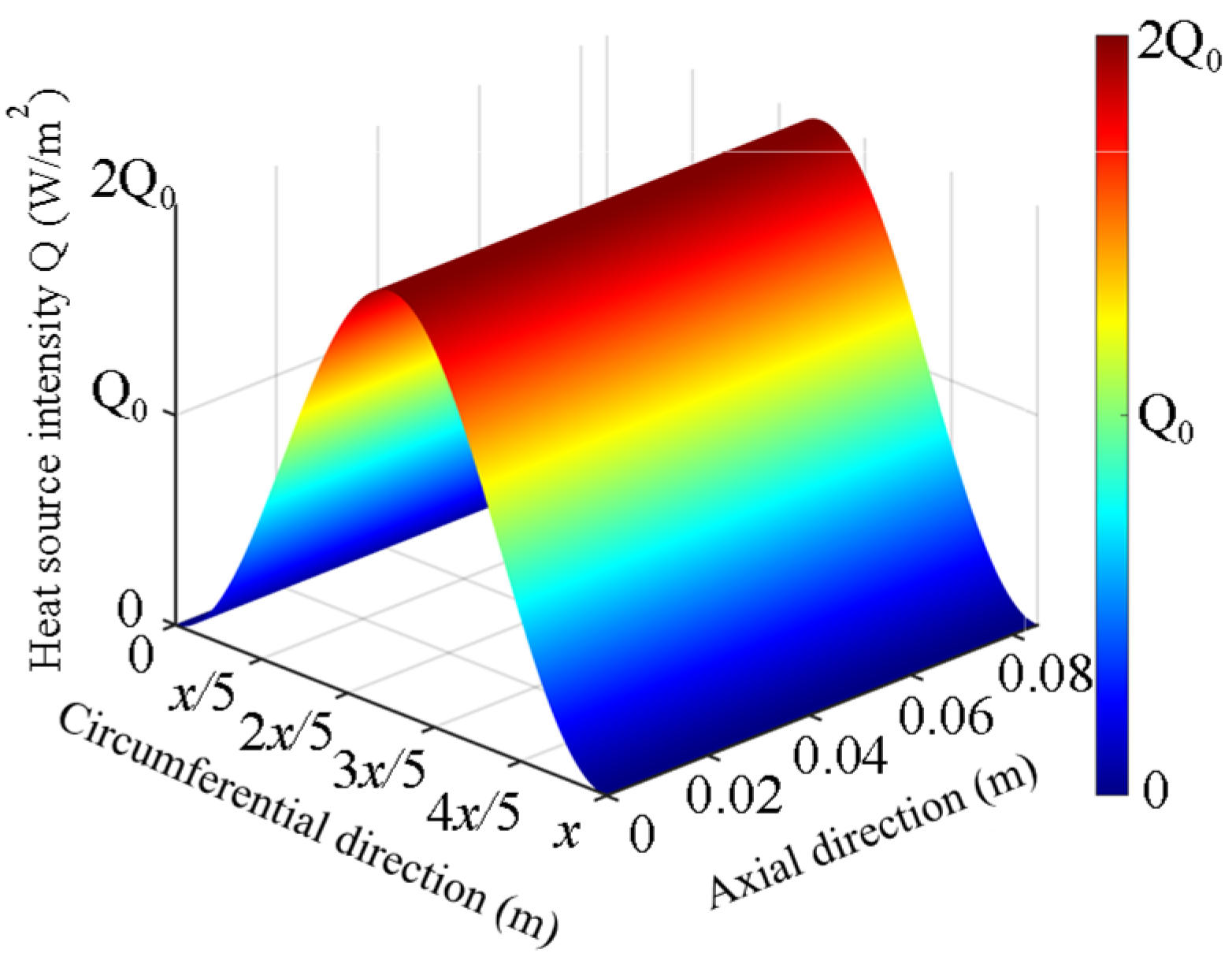
2.4. Sinusoidal Distributed Heat Source Model

This section assumes that the frictional contact heat source between the wheel and the brake shoe follows a sinusoidal distribution, and based on this assumption, a sinusoidal distributed contact heat source model is established. The model assumes that the heat source in the friction contact area varies circumferentially along the wheel tread, exhibiting a sinusoidal waveform. This approach aims to more accurately simulate the distribution characteristics of the contact heat source during the actual friction process. By using this assumption, the spatial variation of the friction heat source can be effectively captured, providing more realistic boundary conditions for subsequent heat conduction analysis. Based on the energy equivalence principle, the formula for the sinusoidal distributed heat source model is shown in Equation (27), and the distribution contour is shown in Figure 4.

$$q_{\sin \text{-}\mathrm{w}}=Q_{\mathrm{w}\text{-}\mathrm{const}}\left(1-\cos {\displaystyle \frac{\overline{V}}{R_{\mathrm{w}}}}x\right)$$

(27)

where $\overline{V}$ is the wheel’s average speed (m/s).

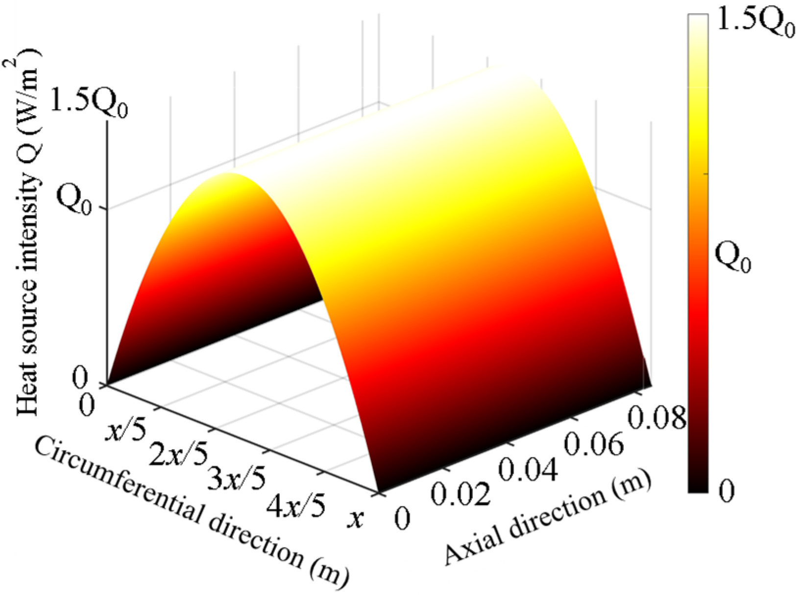
2.5. Parabolic Distributed Heat Source Model

In this section, it is assumed that the friction contact heat source between the wheel and the brake shoe follows a parabolic distribution. Based on this assumption, a parabolic contact heat source model is established to better represent the distribution of heat source within the friction zone. This model simulates how the contact heat source varies across the surface in a parabolic manner, which is closer to the actual distribution found in real-world braking scenarios. Additionally, a moving heat source application method is introduced, where the heat source is dynamically applied to the contact area as it moves along the wheel surface. This method accounts for the temporal and spatial variations of the frictional heat generation process, providing a more accurate representation of the heat flux distribution during braking. The formula for the parabolic distributed heat source model is shown in Equation (28), and the heat source distribution is illustrated in Figure 5.

$$q_{\mathrm{parabola}\text{-}\mathrm{w}}=1.5·Q_{\mathrm{w}\text{-}\mathrm{const}}·\left(1-{\left({\displaystyle \frac{2x}{T}}-1\right)}^2\right)$$

(28)

3. Development of the Wheel–Brake Shoe Finite Element Model

3.1. Structural Parameters

During train operation, the bogie plays a crucial role in supporting the weight of the vehicle and provides guidance through the wheelsets, ensuring the train can smoothly pass over both straight and curved track sections. Figure 6 is a schematic diagram of freight vehicles. Each vehicle typically is equipped with two bogies and four wheelsets, each of which is fitted with a tread braking device. The braking force is provided by a braking force application mechanism, specifically a combination of the braking beam and the brake mechanism (highlighted in blue in Figure 6). During tread braking, the brake shoe on the wheelset applies a normal force F_N to the wheel tread, generating friction to decelerate the wheel and ultimately achieve the braking function of the train. Meanwhile, due to the frictional interaction, the contact area between the brake shoe and the wheel tread rapidly heats up. The heat generated by the friction accumulates continuously, leading to a gradual increase in temperature in this region.

To accurately simulate the interaction process between the brake shoe and the wheel, the geometric parameters of the wheel and brake shoe need to be considered. This study selects the HEZD-type freight train wheel and LH2-type high-friction composite brake shoe, with the specific geometric design parameters shown in

Table 1. Freight wagon wheel/brake shoe design parameters.

Type of Wheel	Outer Radius Ro/(mm)	Inner Radius Ri/(mm)	Thickness of Tread HDw/(mm)
HEZD	420	10	135
Type of brake shoe	Width δ/(mm)	Length Lb/(mm)	Thickness HDb/(mm)
LH2	85	352	40

.

3.2. Mesh Discretization

In this study, the HEZD-type wheel with a diameter of 840 mm is selected as the subject of analysis. Additionally, the LH2-type brake shoe is chosen, representing a typical wheel–brake shoe combination used in braking systems. To precisely replicate this process, a finite element model of the wheel–brake shoe system is developed, incorporating its actual geometric structure. The three-dimensional geometric model of the wheel and brake shoe is shown in Figure 7a, which includes detailed profiles of the wheel and the contact surface of the brake shoe.

Figure 7b shows the process of constructing a three-dimensional finite element model to analyze the frictional behavior between the wheel and brake shoe. To accurately simulate the thermodynamic behavior of the brake shoe during the actual braking process, the model is based on the real geometric structure and uses rigorously defined material parameters for simulation. To effectively capture the heat transfer and distribution during the friction process, the SOLID 70 thermal analysis element in ANSYS 17.0 is used.

To ensure the accuracy of thermal conduction analysis, the three-dimensional finite element mesh of the wheel and brake shoe was divided using hexahedral elements. Particularly in the contact region, the mesh size was further refined to enhance local computational accuracy. The mesh design in the wheel tread region was also refined, with the mesh size set to 1 mm in the axial direction of the brake shoe contact area, enabling better capture of the heat effects generated by friction. Through ANSYS 17.0 simulation, the calculated friction contact area of the brake shoe was approximately 0.025149 m².

The three-dimensional finite element model consists of 228,352 elements and 153,278 nodes. Mesh convergence analysis verified that the model effectively computes the temperature field of the wheel tread and brake shoe contact area, accurately reflecting the thermal effects of heat conduction and friction.

However, the brake shoe friction process involves multiphysics coupling, including material temperature dependence, heat conduction, convection, etc., exhibiting significant nonlinearity. Due to these complex coupling effects, both theoretical analysis and numerical solutions face significant challenges. Under the conditions of long downhill ramps, the train braking time is extended, resulting in prolonged frictional heat generation between the wheel and brake shoe. For simulating the long-term frictional heat generation of the wheel, the three-dimensional model is no longer applicable as its computational load is typically several times that of the two-dimensional model. Therefore, a two-dimensional model was developed in this study to simulate the long-term frictional contact behavior between the wheel and brake shoe and to compute the temperature–time curve for the wheel surface. As shown in Figure 8, the two-dimensional brake shoe friction thermal analysis model adopts a two-dimensional structure to obtain the temperature–time curve along the wheel tread circumference and radial direction. The thermal analysis model uses PLANE 77 elements for transient thermal analysis. The implicit Crank–Nicolson numerical integration method is used to solve the equations, and the Newton–Raphson method is applied iteratively at each time step to solve the nonlinear system of equations, updating the temperature field solution until convergence is achieved. The finite element model consists of 28,800 elements and 86,880 nodes. To ensure the accuracy of the temperature field calculation, mesh refinement is applied within a 10 mm radial region of the wheel tread, with a radial mesh size of 0.5 mm. A comparison study of the temperature–time curves between the two-dimensional and three-dimensional models, along with experimental validation, has been conducted in [48], with the maximum temperature difference between the two models being 2.5%, less than 5%, ensuring good accuracy.

3.3. Heat Source Application Methods

In the actual friction process between the wheel and brake shoe, a contact–separation–recontact cycle occurs. The moving heat source method can more accurately simulate this process. Figure 9 shows the distribution of heat flux load in the wheel circumferential direction during wheel rotation. In the figure, v represents the direction of the wheel’s rotational velocity. For instance, when considering a modified Gaussian-type friction heat source between the wheel and brake shoe, a heat source is generated within the contact length L_b at time T_i. This paper proposes several heat flux load distribution models, including constant-type, modified Gaussian distribution-type, sinusoidal-type, and parabolic-type heat flux distribution forms. As the wheel rotates in the direction of velocity v, the circumferential friction position between the wheel and brake shoe continuously changes, which is equivalent to the wheel–brake shoe heat source moving circumferentially along the wheel tread. In Figure 9, the time T_i+1 corresponds to the next moment after T_i, and the difference between T_i+1 and T_i represents the time step in the finite element analysis. As the wheel continuously rotates, the heat source moves circumferentially along the wheel tread, as at times T_i+2, T_i+3, and so on, until time T_i+n.

For the heat source application methods in both 2D and 3D wheel finite element models, the application method is consistent, with both adopting the ANSYS 17.0 tabular load construction method for application. In the following, the heat source model application method for the 3D wheel finite element model will be introduced.

In particular, the choice of load time step has a significant impact on the calculation results as the time step directly determines the accuracy of the heat flux load transfer process and the precision of the temperature field and thermal stress field distributions.

To ensure the accuracy of the simulation results, this paper adopts a sufficiently small time step. At a vehicle speed of 60 km/h, after optimization, the time step is set to 0.0013188 s. This time step configuration enables a more precise capture of frictional heat accumulation and transfer during wheel–brake shoe contact, resulting in a more realistic distribution of the frictional temperature field.

Due to the symmetry of the wheel tread, one-quarter of the wheel’s area is selected as the research object, and the mathematical expression of the heat source application formula is derived accordingly. To facilitate analysis, a global coordinate system (xOy) is established in the circumferential plane of the wheel, and a local coordinate system (zO′ρ) is established on the wheel tread, as shown in Figure 10. In the xOy coordinate system, the initial position of the heat source is θ₀, and it moves along the circumferential direction. The angular velocity of the wheel is ω, and at any given moment, the wheel’s rotation angle is ωt_i, which determines the position of the heat source on the wheel tread. To describe the trajectory of the heat source, angular variation relations in polar coordinates are used. In the local coordinate system zO′ρ, the ρ-axis indicates the central position of the heat source and is perpendicular to the z-axis, ensuring consistency between the physical contact model of the heat source and the wheel tread.

In Figure 10b, the red area represents the contact area between the wheel tread and the brake shoe. To simplify the analysis, it is assumed that the heat source is uniformly distributed along the wheel’s axial direction (i.e., the AA′ direction) and that this distribution is independent of the wheel’s rotation. The contact width H_b represents the effective width of the contact region between the wheel tread and the brake shoe, typically the contact width between the wheel tread and the brake shoe. This assumption reasonably simplifies the model and aids in analyzing the distribution characteristics of the heat flux and its transmission behavior on the wheel tread.

Moreover, considering the motion characteristics of the friction heat source, this paper further derives the variation law of the heat source application position with the wheel’s rotation angle and quantitatively analyzes the heat distribution of the heat source at different moments. This method enables accurate simulation of the heat flux variation in the friction process between the wheel and the brake shoe, providing a foundation for subsequent calculations of the temperature field and thermal stress field.

As shown in Figure 10a, in the zO′ρ coordinate system, within the time step t_i, the center of the heat source moves from O₁ to O₂, covering a distance H_i:

$$H_i=\left(\omega t_i-{\theta }_0\right)R_{\mathrm{w}}$$

(29)

The application of heat flux is given by the following equation:

$$q=\left\{\begin{array}{cc}{q}_{\mathrm{w}}& \left(z,\rho \right)<S\mathrm{r}\\ 0& \left(z,\rho \right)<S\mathrm{e}-S\mathrm{r}\end{array}\right.$$

(30)

In the equation, S_e represents the outer surface of the wheel, S_r denotes the contact surface between the wheel and the brake shoe, and q_w is the heat flux transferred into the wheel. At time t_i, the contact surface area S_r between the wheel and the brake shoe is given by:

$$S\mathrm{r}:\left(\rho ·R_{\mathrm{w}}-H_i\right)·H_{\mathrm{b}}\le L_{\mathrm{b}}·H_{\mathrm{b}}$$

(31)

$$S\mathrm{r}:\left(\rho R_{\mathrm{w}}-\omega t_i{R}_{\mathrm{w}}+{\theta }_0{R}_{\mathrm{w}}\right)·H_{\mathrm{b}}\le L_{\mathrm{b}}·H_{\mathrm{b}}$$

(32)

$$S\mathrm{r}:\left(\rho -\omega t_i+{\theta }_0\right)\le L_{\mathrm{b}}/R_{\mathrm{w}}$$

(33)

In the equation, H_b represents the effective contact width of the brake shoe (m).

3.4. Thermal Analysis Boundary Conditions

During the tread braking process, the thermal analysis of the wheel–brake shoe friction system involves three types of boundary conditions. As shown in Figure 11, the diagram illustrates the boundary conditions of the tread braking system. The diagram highlights the regions influenced by these boundary conditions, where the red areas represent heat accumulation regions, and the blue areas indicate heat dissipation regions.

(1)

Initial temperature boundary condition: Defines the initial temperature of the wheel and brake shoe, which is typically set to the ambient temperature to simulate thermal equilibrium before braking begins.

(2)

Thermal input boundary condition: The heat generated by friction is applied to the contact surface between the wheel and the brake shoe. This heat input is typically defined using heat flux.

(3)

Thermal output boundary condition: Heat dissipates from the system, primarily through convective heat transfer and thermal radiation acting on the wheel surface.

3.4.1. Initial Conditions

In this study, the temperature distribution of both the wheel and the brake shoe is assumed to be uniform at the initial moment, equating to the ambient temperature. To streamline the thermal analysis calculations, the ambient temperature, denoted as T_A, is established as a constant. This value is designated as the initial temperature condition for the finite element model. By doing so, the initial state of the model is meticulously aligned with actual operating conditions, thereby enhancing the accuracy and reliability of subsequent thermal analyses.

$$t\left(x,y,z,0\right)=T_{\mathrm{A}}$$

(34)

3.4.2. Thermal Input Boundary Conditions

Equation (35) presents the expression for the thermal input boundary condition. The construction of friction work and power density for different heat source methods has been completed in Section 2, and the application method of the heat source is covered in Section 3.3. Therefore, the heat input boundary conditions will not be discussed in detail in this section.

$$-\lambda {\displaystyle \frac{\partial T}{\partial n\prime }}{|}_{S_r,t>0}=q+h(T-T_{\mathrm{A}})+\epsilon \sigma (T^4-{T_{\mathrm{A}}}^4)$$

(35)

In the equation, n′ refers to the normal surface of the wheel/brake shoe.

3.4.3. Thermal Output Boundary Conditions

During the operation of the vehicle, thermal energy is transferred from the wheel and brake shoe to the ambient air via heat exchange processes. The heat dissipation boundary conditions for the wheel and brake shoe are defined as follows:

$$-\lambda {\displaystyle \frac{\partial T}{\partial n}}{|}_{S_{\mathrm{e}}-S_r,t>0}=h(T-T_{\mathrm{A}})+\epsilon \sigma (T^4-{T_{\mathrm{A}}}^4)$$

(36)

Although the contribution of thermal radiation is relatively minor, its nonlinear characteristics would substantially increase computational complexity. For this reason, heat radiation is not taken into account in this study, as supported by references [28,49]. In the field of fluid dynamics, the Reynolds number serves as a critical dimensionless parameter to describe the regime of fluid flow, representing the ratio of inertial forces to viscous forces. To precisely model the wheel’s motion during braking, the Reynolds number (Re) is expressed as a function of the wheel’s circumferential velocity, (V_c).

$$Re={\displaystyle \frac{2R_i{V}_{\mathrm{c}}}{{\zeta }_{\mathrm{a}}}}$$

(37)

In the equation, ξ_a is the air kinematic viscosity (m²/s), V_c is the wheel’s circumferential speed (m/s), and R_i is the radius at a specific point on the wheel.

In the thermal analysis of tread braking systems, the Prandtl number (Pr) is a dimensionless parameter that characterizes the relationship between thermal diffusivity and momentum diffusivity. It is a key factor in assessing the efficiency of heat transfer between the airflow and the wheel surface. The Prandtl number is defined as:

$$Pr={\displaystyle \frac{{\rho }_{\mathrm{a}}{\xi }_{\mathrm{a}}{c}_{\mathrm{a}}}{{\lambda }_{\mathrm{a}}}}$$

(38)

In the equation, ρ_a is the air density (kg/m³), c_a is the specific heat capacity of air (J/(kg·°C)), and λ_a is the thermal conductivity of air (W/(m·°C)).

The Nusselt number (Nu) serves as a dimensionless parameter to evaluate the effectiveness of convective heat transfer within the fluid boundary layer. It is intrinsically linked to both the Reynolds number and the Prandtl number and is widely employed to characterize the thermal interaction between the airflow and the wheel surface. The Nusselt number is calculated as follows:

$$Nu=0.3+{\displaystyle \frac{0.62\sqrt[2]{Re}\sqrt[3]{Pr}}{\sqrt[4]{1+{\left(\frac{0.4}{Pr}\right)}^{\frac{2}{3}}}}}{[1+{({\displaystyle \frac{Re}{282000}})}^{{\displaystyle \frac{5}{8}}}]}^{{\displaystyle \frac{4}{5}}}$$

(39)

The convective heat transfer coefficient can be determined based on well-established methodologies documented in the literature [50,51].

$$h_{\mathrm{a}}={\displaystyle \frac{Nu{\lambda }_{\mathrm{a}}}{2R_{\mathrm{w}}}}$$

(40)

In the equation, h_a represents the convective heat transfer coefficient (W/(m²·°C)).

3.5. Material Parameters

The material used for the wheel in this study is CL60 steel, while the brake shoe is made from a resin-based, high-friction composite material. According to reference [52], tensile tests on CL60 steel were performed using a high-temperature creep testing machine to assess its mechanical and thermal properties under varying temperature conditions. These tests covered a wide range of temperatures and measured key parameters, including stress–strain behavior, Young’s modulus, yield strength, tensile strength, thermal expansion coefficient, and thermal conductivity. The thermophysical parameters of the material play a critical role in the temperature evolution and distribution. Based on the experimental results presented in reference [52],

Table 2. Thermophysical properties of CL60 steel material.

Temperature (°C)	Specific Heat (J/(kg·°C))	Thermal Conductivity (W/(m·°C))
26	470	51.0
100	490	49.0
200	530	45.0
300	570	42.0
400	620	38.0
500	680	35.0
600	790	32.0

provides the detailed thermal properties of CL60 steel at different temperature levels. It can be observed that as the temperature increases, the specific heat capacity gradually increases, while the thermal conductivity gradually decreases.

4. Results and Discussion

4.1. Theoretical Validation of the Heat Source Model

To evaluate the effectiveness of different heat source models, a comparative analysis was conducted against the numerical simulation results reported in references [27,53]. The simulation conditions used in the literature are summarized in

Table 3. Operating parameters for comparative validation of heat source models.

Freight Wagon Weight M (t)	The Speed of Freight Wagon Vv (km/h)	The Slope Gradient s (‰)	Friction Coefficient μwb	The Normal Force on the Brake Block FN (kN)	Ref.
80	60	21	0.14	13.84	[27,53]

. Using the same material parameters as those in the references and applying a two-dimensional finite element (FE) model of the wheel, we employed the constant heat source model proposed in this study for comparison.

Figure 12 illustrates the temperature evolution at the wheel tread during drag braking. Under the specified service conditions, the train traveled approximately 250 m, and the tread surface temperature rose to around 59.6 °C. The blue curve in the figure represents the temperature–time history fitted from the numerical results in reference [53], while the red data points are extracted from reference [53] based on 10 sampling points taken along the curve presented in reference [27], serving as additional validation. Figure 12 presents a comparative analysis of the calculated tread temperatures during drag braking against the results from references [27,53].

The comparison shows that the temperature–time evolution obtained using our FE-based heat source model aligns well with the trends observed in references [27,53]. The peak temperature differs by only 0.6 °C from that in reference [53] and by 3.6 °C from that in reference [27]. These results demonstrate the accuracy and reliability of the proposed finite element model. In conclusion, the model proposed in this study demonstrates good accuracy in predicting the thermal behavior of the wheel tread under continuous drag braking conditions on long slopes.

4.2. Comparison of Heat Source Models and Experimental Analysis

As stated in reference [27], experimental studies on the tread braking process over long and steep gradients are currently limited, and experimental data are rarely reported. Recently, reference [54] described an experimental study that measured wheel tread temperature during braking on long downhill ramps. The wheel material used in the experiment was CL60 steel, with a diameter of 840 mm, while the brake shoe was made of a resin-based composite material, having a width of 85 mm. These dimensions are consistent with those used in this study. The experiment was conducted using the German-imported BD2500/15000 test stand, which simulates 1:1 vehicle braking power. The test stand is capable of reaching a maximum rotational speed of 2500 rpm, a maximum braking torque of 15,000 Nm, and a rated motor power of 450 kW, making it suitable for brake thermal fatigue testing.

The experiment was conducted in pressure control mode, with the braking pressure set at 3 kN and the train’s speed fixed at 70 km/h. The initial temperature was set to 50 °C. Under the steady braking condition on the long downhill ramp described in this study, friction tests were conducted between the wheel and brake shoe. After 100 s of friction, the average wheel tread temperature reached 112 °C.

4.2.1. Time-Domain Response of Circumferential Temperature on the Wheel Tread

To compare and analyze with the experimental results, simulations are conducted under the same conditions as the experiments in this section. The temperature–time response along the circumferential direction of the wheel tread is presented in a three-dimensional color contour map. The temperature–time response curves of nodes at different angles along the circumferential direction of the wheel tread are shown in Figure 13. According to the calculation results, the highest temperature on the wheel tread obtained from the constant heat source model is 119.80 °C, from the modified Gaussian distribution heat source model is 121.18 °C, from the sine distribution heat source model is 119.85 °C, and from the parabolic distribution heat source model is 118.70 °C. The temperature results, in descending order, are as follows: modified Gaussian distribution heat source, sine distribution heat source, constant heat source, and parabolic distribution heat source. To facilitate the analysis, the temperature difference percentage is defined by the following formula:

$$\varsigma ={\displaystyle \frac{T\mathrm{s}-T\mathrm{e}}{T\mathrm{e}}}\times 100\%$$

(41)

where T_s represents the highest temperature of the wheel tread calculated using the four heat source methods (°C), and T_e represents the average temperature of the wheel tread obtained from experimental calculations (°C).

Compared to the average temperature result of 112 °C obtained from experimental calculations of the wheel tread, the temperature difference between the experimental results and the four types of heat sources is a maximum of 8.2% and a minimum of 6.0%. It should be noted that 112 °C is the average temperature calculated for the wheel tread. Due to the thermal elastic instability phenomenon induced by friction, the highest temperature measured in the experiment was higher than this value. Therefore, considering the relatively small temperature differences between the results calculated by the various heat source models and the experimental values, it can be concluded that the heat source models proposed in this paper satisfy the requirements for calculating frictional heat generation between the wheel and brake shoe on long downhill ramps.

Among the four models, the modified Gaussian heat source model results in a wheel tread temperature that is 8.2% higher than the experimental average temperature, more accurately reflecting the thermal elastic instability induced by friction between the wheel and brake shoe. This model aligns better with the actual physical phenomenon of frictional heat generation. The sine, constant, and parabolic models show decreasing temperatures in this order. This is due to the different degrees of heat flux concentration in these models, indicating that as the concentration of heat flux decreases, the local temperature peak also decreases.

In the simulation, the key to better comparing experimental results lies in how the local excitation of frictional heat and thermal elastic instability are described. Frictional contact often leads to localized hotspots and rapid temperature changes, especially when thermal elastic instability is excited, where high-temperature regions are confined to certain areas of the friction contact zone. For the modified Gaussian and sine distribution models, these two models better represent this phenomenon by concentrating the heat input. In contrast, for the constant and parabolic distribution models, although the overall mean temperature may be close to the experimental average (112 °C), their simulation results lack the local high-temperature excitation mechanism, which limits their ability to reflect local high-temperature phenomena. Additionally, from the temperature–time response contour map, it is clearly visible that, compared to the constant distribution heat source, the maps generated using the modified Gaussian and sine distribution heat sources show more distinct localized heating phenomena. The calculation results better match the actual wheel–brake shoe frictional heat coupling process, with the modified Gaussian distribution model highlighting this physical phenomenon most effectively.

The reason is that, when heat flux is locally concentrated, the steep thermal gradient leads to faster heat conduction within the local material, resulting in higher temperature peaks at the moment of contact. This localized high-temperature region then diffuses heat to the surrounding area, creating a clear hotspot structure in the temperature–time response contour map. In the modified Gaussian and sine models, the higher local heat flux causes a rapid local temperature rise, which then diffuses and equilibrates through thermal conduction, forming a more layered temperature field. In contrast, the constant and parabolic models, due to their more evenly distributed heat input, result in a smoother heat distribution across the entire tread, with less noticeable local temperature increase and a lack of significant thermal gradient changes, leading to weaker layering in the contour map. In the temperature–time response contour map for the wheel tread, using Gaussian and sine heat sources allows for a clearer display of the temperature inhomogeneity along the wheel tread’s circumferential direction. This aligns with the actual friction process, where local contact conditions, pressure fluctuations, and material heterogeneity vary. On the other hand, the constant heat source fails to reflect this layering and localized hotspots, indicating its limitations in capturing the thermal elastic instability induced by frictional heat.

4.2.2. Time-Domain Response of Radial Temperature on the Wheel Tread

A comparative analysis of the temperature–time domain distribution results in the radial direction was conducted for the four heat source methods. According to existing studies, the initiation of thermal cracks usually occurs within a depth of 10 mm below the wheel tread surface [55]. Therefore, this study focuses on analyzing the temperature distribution within this 10 mm depth range for different heat source methods. Specifically, for the four heat source models—modified Gaussian distribution, sinusoidal distribution, constant heat source, and parabolic distribution—it focuses on the calculated temperature variation at the maximum temperature point on the wheel tread in the radial direction. As shown in Figure 14, the radial temperature variation within the 10 mm range is as follows: for the constant heat source, it ranges from 119.80 °C to 101.83 °C; for the modified Gaussian distribution, from 121.18 °C to 100.28 °C; for the sinusoidal distribution, from 119.85 °C to 100.26 °C; and for the parabolic distribution, from 118.70 °C to 100.21 °C.

For the modified Gaussian distribution heat source, the surface temperature reaches its peak at 121.18 °C, forming a steep temperature gradient. This rapid heat conduction in the radial direction reduces the temperature at a depth of 10 mm to approximately 100.28 °C. The sinusoidal distribution heat source also has a high heat flux in the central region, but its distribution is smoother, leading to a slightly lower surface temperature (119.85 °C), with a temperature gradient weaker than that of the Gaussian distribution heat source, and the temperature at 10 mm drops to approximately 100.26 °C. In contrast, the constant heat source assumes a uniform heat flux distribution across the entire contact area, leading to a less pronounced hotspot effect. This results in a relatively uniform surface temperature of 119.80 °C, a gentle temperature gradient, and the slowest radial temperature decay, with the temperature at 10 mm dropping only to 101.83 °C. The parabolic distribution heat source, while accounting for a higher center and lower edges, exhibits a lower degree of energy concentration than the previous two models. Consequently, it produces the lowest surface temperature (118.70 °C) and a temperature of approximately 100.21 °C at 10 mm.

According to Fourier’s law of heat conduction, the increase in local temperature is proportional to the heat flux, and the rate of temperature decay is determined by the material’s thermal conductivity and the local temperature gradient. The modified Gaussian distribution heat source, due to the large local temperature gradient formed at the contact surface, facilitates the diffusion of heat with a larger gradient toward the wheel interior, resulting in a significant temperature decay. The sinusoidal distribution heat source, while maintaining local hotspots, has a milder temperature gradient. The constant and parabolic distributions, due to their uniform heat input, lead to a slower temperature decay during heat transfer, resulting in a more balanced temperature distribution within the wheel.

The numerical simulation results show that the modified Gaussian distribution heat source not only achieves the highest temperature at the contact surface but also forms a significant radial temperature gradient, which is more in line with the actual physical process of frictional heat generation. The sinusoidal distribution heat source strikes a balance between localized energy concentration and smooth distribution. The constant and parabolic distributions, however, due to their overly uniform energy input, reflect the overall temperature field but fail to reproduce local high temperatures and gradients, making them less effective in predicting thermal crack initiation locations.

4.3. The Temperature Field Distribution of the Wheel Tread

This section calculates and analyzes the temperature distribution of the wheel tread during the frictional heating process between the wheel and the brake shoe, comparing different heat source models. The study examines the temperature distribution of modified Gaussian, sinusoidal, uniform, and parabolic heat sources. The temperature field distribution on the wheel tread is compared after 1 full wheel rotation (Figure 15) and after 74 rotations (10 s) (Figure 16).

After one wheel rotation, the tread temperature exhibits an irregular distribution with prominent peaks. Under constant-speed braking conditions, due to relatively low heat input and convective heat dissipation, the tread temperatures calculated for constant, modified Gaussian, sinusoidal, and parabolic heat sources are 55.52 °C, 55.95 °C, 55.72 °C, and 55.46 °C, respectively. Among them, the modified Gaussian heat source produces the highest peak temperature, allowing for a more accurate capture of local temperature extremes and best reflecting the thermoelastic instability induced by friction.

After 74 wheel rotations, the tread temperature still exhibits an irregular distribution. The contour plot reveals that, compared to the constant heat source, the modified Gaussian, sinusoidal, and parabolic heat sources result in more pronounced local temperature peaks, aligning better with the physical characteristics of actual tread braking processes. Among these, the modified Gaussian heat source most accurately represents the real frictional heating phenomenon.

4.4. Discussion

Figure 17 shows the power density distribution of the wheel tread, calculated using different heat source models on the same bottom surface area. Based on the energy equivalence principle, the areas enclosed by the four curves and the horizontal axis of the coordinate system are equal. It is observed that the modified Gaussian distribution heat source has the highest power density peak, followed by the sine distribution, the constant heat source, and the parabolic distribution.

Figure 18 illustrates the temperature–time history at a specific node on the wheel tread. The temperature–time curve is flat during the initial phase as the node does not yet experience the heat boundary load, and the moving heat source has not yet reached that node. The figure shows the temperature–time history over three cycles for this node. During one cycle, when the wheel tread node passes through the wheel–brake shoe contact zone, the heat flux causes the temperature to rise. Away from the contact zone, convective heat exchange leads to a temperature drop, resulting in alternating temperature fluctuations. The modified Gaussian distribution heat source exhibits the most rapid temperature increase, reaching the highest peak temperature in the shortest time, followed by the sine distribution. The parabolic distribution ranks third, while the constant heat source results in the lowest temperature rise.

The reasons for these phenomena mainly lie in the degree of local heat flux concentration, heat conduction and diffusion effects, the spatiotemporal characteristics of energy accumulation and dissipation, and the differences in finite element responses in numerical simulations. According to Fourier’s law of heat conduction, local temperature changes are influenced by the magnitude and distribution of heat flux. Different heat source distributions determine the spatial distribution of a heat flux in the contact region, thus affecting the amplitude and rate of local temperature increase.

During the temperature rise phase, the modified Gaussian distribution heat source exhibits sharp peaks and fast decay characteristics, with the highest heat flux at the contact center and rapid decay at the edges. This localized concentration effect causes rapid energy accumulation at the contact center, resulting in a rapid increase in temperature and a shorter time to reach the peak. The sine distribution heat source has a smoother change in heat flux, with a less sharp peak than the modified Gaussian distribution, resulting in a lower energy concentration and, thus, a lower rate and amplitude of temperature rise. The parabolic distribution has a heat flux that decreases from the center, leading to a more uniform energy distribution and a more gradual temperature rise, taking longer to reach the highest temperature. The constant heat source assumes a uniform distribution of heat flux, with no clear hotspot, resulting in the smallest temperature rise and the longest time to reach the highest temperature.

During the temperature drop phase, the modified Gaussian distribution heat source shows the fastest temperature rise at the center and a high heat diffusion rate, leading to a quicker temperature drop. The sine and parabolic distributions have more uniform temperature distributions, with slower heat diffusion, leading to a more gradual temperature decrease. The constant heat source has the most uniform heat flux, leading to the most gradual temperature rise and fall.

Furthermore, from the perspective of thermal inertia, the modified Gaussian distribution heat source has the highest energy input per unit area, causing the local thermal inertia to result in the fastest temperature rise, and due to rapid heat diffusion, the temperature drop is also steeper. The sine and parabolic distribution heat sources, with more uniform energy input, lead to a longer local thermal response time, making both the temperature rise and drop more gradual. The constant heat source, with the most uniform heat flux and temperature field distribution, has the most pronounced thermal inertia effect, resulting in the most gradual temperature rise and drop.

During short contact periods, the local high heat flux (such as modified Gaussian-type) generates significant temperature gradients within the contact zone, inducing faster local heat conduction and leading to a rapid temperature rise. In contrast, the constant heat source has a smaller temperature gradient due to its uniformity, resulting in slower heat diffusion. The sine and parabolic distributions fall between the two. The transient heat conduction analysis in the finite element model reflects this, where the form of the local heat source distribution determines the rate of heat transfer and accumulation inside the material.

Overall, the different distribution forms of the four heat sources primarily influence the amplitude of temperature rise and response time at individual nodes by altering the concentration of local heat flux density, the temperature gradient, and the transient heat conduction process.

In the actual wheel–brake shoe friction process, thermoelastic coupling effects may cause local thermal excitation instability, leading to significant instantaneous temperature fluctuations. The modified Gaussian distribution heat source, due to its highest concentration, better captures this instantaneous thermal excitation phenomenon, and its results match the observed local temperature “overshoot” more closely.

In engineering applications, the Gaussian and sine distribution heat sources more accurately reflect the actual frictional heat generation, while the parabolic and constant heat sources, due to their overly uniform energy distribution, may underestimate local temperature rise. Therefore, in braking system design, if the effects of local high temperatures on material performance (such as thermal fatigue or thermal cracking) need to be considered, using Gaussian or sine distribution heat sources for analysis will yield more accurate results.

The rate of change of the time–temperature gradient reflects the instantaneous rate of temperature change and influences the thermoelastic instability induced by frictional heat. The formula for defining the rate of change of the time–temperature gradient is:

$$G={\displaystyle \frac{\Delta T}{\Delta t}}$$

(42)

where ΔT is the temperature change over a short period (°C), and Δt is the corresponding time interval (s).

The percentage increase in the temperature gradient change rate is calculated using the formula:

$$\varphi ={\displaystyle \frac{G\mathrm{g}-G\mathrm{c}}{G\mathrm{c}}}\times 100\%$$

(43)

where G_g is the temperature gradient change rate for the modified Gaussian distribution heat source, and G_c is the temperature gradient change rate for the constant distribution heat source.

Calculations show that the temperature gradient for the modified Gaussian distribution heat source is 81 °C/s, while the temperature gradient for the constant distribution heat source is 58 °C/s, resulting in a 40% increase in the temperature gradient change rate.

5. Conclusions

This study addresses the frictional heat generation between the wheel and brake shoe under long and steep slope conditions. Based on the energy equivalence principle, four heat source models are proposed, and their applicability and accuracy are validated through comparison with experimental data. The main conclusions are as follows:

(1)

The four heat source models (modified Gaussian distribution, sinusoidal distribution, constant distribution, and parabolic distribution) are capable of simulating the frictional heat generation between the wheel and brake shoe effectively. The computed temperature responses are in good agreement with the experimental measurements, with temperature differences ranging from 6.0% to 8.2%, demonstrating the effectiveness and reliability of the proposed methods under long and steep slope conditions.

(2)

Among the four models, the modified Gaussian distribution heat source, with its sharp central peak (the heat flux peak is 2.82 times that of the constant heat source model) and rapid decay characteristics, can more accurately capture the non-uniform distribution of heat flux in the contact zone. This results in a temperature peak that is 8.2% higher than the average temperature from experimental data and creates a steeper temperature gradient (the gradient change rate is approximately 40% higher than the constant heat source), better simulating the local “hotspot” effect. This model more closely approximates the actual situation in terms of temperature peak and distribution hierarchy, showing higher computational accuracy.

(3)

In actual braking processes, the contact state between the wheel and brake shoe exhibits spatial and temporal non-uniformities. Local high-temperature regions and thermoelastic instability play important roles in the occurrence of thermal fatigue and thermal cracking. The proposed new heat source model fully accounts for the spatial and temporal non-uniformities of heat flux during the wheel–brake shoe contact, effectively describing local temperature rise and accurately predicting frictional heat transfer and thermoplastic instability. The findings can be used to optimize the finite element models of braking systems, improve the accuracy of wheel thermal damage predictions, and reduce the risk of failure in brake components due to thermal fatigue, thereby providing solid technical support for the safety and durability of braking systems in long and steep slope railways and heavy-load transportation.

In summary, the new wheel–brake shoe friction heat source method proposed in this study has significant advantages in capturing the local high-temperature “overshoot” phenomenon, reproducing the temperature domain distribution hierarchy, and reflecting thermoelastic instability. It provides a solid theoretical basis and technical support for further optimizing finite element models of long and steep slope braking systems and predicting wheel thermal damage. Moreover, the proposed model can be extended to other braking systems (e.g., disc brakes [56]) through appropriate modifications to the geometry and boundary conditions.

However, several key issues require further investigation to optimize the heat source model and enhance its engineering applicability.

(1)

Future work will consider experimental comparisons involving thermal stress, strain, and material damage, as well as refine the heat source distribution by integrating experimental data and implementing adaptive corrections to further enhance the proposed model. By fitting the experimentally measured temperature field data, a dynamic heat source model that better reflects the actual characteristics of frictional heat generation can be developed.

(2)

The present study is primarily conducted under idealized conditions. However, in practical braking scenarios, the wheel–brake shoe contact state may be influenced by factors such as friction material wear, ambient temperature, humidity, and braking force fluctuations. To improve model adaptability to real-world conditions, future studies should incorporate more complex environmental variables, such as dynamic contact conditions and the evolution of surface roughness.

From an engineering application perspective, the proposed modified Gaussian distribution heat source model demonstrates superior accuracy in capturing localized high-temperature peaks. This provides strong theoretical and computational support for optimizing finite element modeling of braking systems and improving thermal damage prediction accuracy. Future research could explore the broader application of this model in other railway and heavy-haul transportation systems, such as metro trains. Additionally, optimizing braking system design to further enhance thermal stability, extend component lifespan, and ensure the safety of long-gradient and heavy-load railway operations remains an important avenue for future work.