Abstract
Uncontrolled wear in complex multiphysics systems can cause catastrophic failures, prompting the development of empirical methods and numerical prediction models for managing system lifetimes. This study introduces a novel approach for predicting wear on lubricated sliding surfaces by integrating rough contact mechanics into a nonlocal function with a non-uniform distribution. The model considers the sliding speed, contact area, fluid pressures, lubricant properties, and surface roughness. It employs a mixed elastohydrodynamic lubrication (mixed EHL) model to simulate lubrication and wear, using a multiscale roughness model to adjust the parameters based on the wear evolution. Validated against journal bearing data, the model accurately predicted wear rates and depths, revealing distinct roughness variations depending on the lubricant viscosity.
1. Introduction
The interaction between moving surfaces has been a critical concern in various fields since the invention of the wheel, mainly due to its implications for the efficiency and durability of engineering systems. Nowadays, this subject extends to various applications, from human joint implants to thrust bearings in submarines. The effective management of tribological interactions is essential to prevent premature wear, an early need for maintenance, and operational inefficiencies, with uncontrolled wear evolution potentially resulting in catastrophic failures. Therefore, empirical experimentation methods and numerical prediction models have been developed to manage the finite lifetime of systems in various applications [1,2,3,4,5,6,7]. Empirical methods have long been employed to understand the underlying wear mechanisms in tribosystems, and this approach remains relevant, particularly for addressing new challenges in green tribology and biotribology. Conversely, numerical methods for tribology and wear prediction have consistently been developed and validated using experimental results. Wear prediction initially relied on empirical laws correlating the wear rates under different contact conditions, which later led to the development of complex mathematical models incorporating various tribological parameters [8,9,10,11,12].
Nonlocal continuum field theories [13] provide a mathematical framework for coupling tribological phenomena across scales of different lengths, including contact mechanics and wear-related processes. Several researchers have used these theories in damage models to distribute specific variables over an influence area, thus avoiding local concentrations or singularities that fail to represent the actual distribution and magnitude of quantities involved in physical interactions [14,15,16,17,18,19]. The direct validation of these models is often unfeasible, as many tribological applications do not allow for direct measurements. Consequently, tribological studies typically validate these methods by assessing their impact on macroscopic geometrical changes, such as wear volume removal, crack propagation, or tribofilm growth, which can be measured after testing. The present contribution proposes a novel approach for predicting wear on lubricated sliding surfaces by integrating rough contact mechanics into a nonlocal function with a non-uniform distribution.
Proper surface roughness characterization is essential for accurately predicting the friction and wear under boundary and mixed lubrication conditions [20,21]. Numerous experimental investigations have demonstrated the significant transformation of the surface topography after wear, where the amount and distribution of the material removed changed drastically. This phenomenon is crucial when simulating tribological contacts under severe conditions, as discussed by several authors [22,23]. This work introduces a novel procedure that accounts for variations in roughness in response to the wear evolution of the contact surfaces at the microscale and its macroscopic effect.
Journal bearings are widely used in industrial machinery, internal combustion engines (ICEs), power generation turbines, and other applications due to their high load-carrying capacity, low friction, noise and vibration reduction, ability to accommodate shaft misalignment, and long service life at moderate to high rotational speeds. This study evaluated the effectiveness of the proposed wear model in predicting wear in ICE journal bearings, where lubricant rheology plays a critical role due to the high shear stress and film pressures involved [24,25,26,27,28]. Consequently, the lubrication regime and bearing performance are significantly influenced by the rheological properties of the lubricant and surface roughness characteristics.
The research on elastohydrodynamic lubrication and surface roughness has advanced significantly over the past several decades, as evidenced by the seminal work of Xu and Sadeghi [29], Morales-Espejel [30], Ai and Cheng [31], and Sadeghi and Sui [32], along with the broader body of research they have influenced. These studies collectively underscore the critical importance of considering the surface roughness, thermal effects, transient behaviour, and lubricant compressibility in the analysis of EHL contacts. The field has moved from using simplified models to more sophisticated approaches that incorporate realistic surface topographies and multiple interacting physical phenomena, driven by the increasing demands on the performance and reliability of lubricated mechanical components.
Despite the considerable progress, several avenues remain for future research. The improved modelling of the boundary and mixed lubrication regimes, where both the fluid film and asperity contact play a significant role, is crucial for a more accurate prediction of the friction, wear, and fatigue life. Further investigation into the effects of the non-Gaussian surface roughness characteristics often found in real engineering surfaces is needed to better understand their impact on EHL performance. Moreover, developing more efficient and accurate numerical methods for solving coupled thermo-elastohydrodynamic problems with complex surface topographies remains an ongoing challenge. Studies on the influence of lubricant rheology, particularly piezoviscous and non-Newtonian behaviours, in conjunction with the surface roughness under various operating conditions, are also warranted. Research into the long-term effects of surface roughness evolution due to wear or running-in on the EHL performance and component life is essential for predicting the durability of mechanical systems. Addressing the challenges in obtaining and utilizing accurate, high-resolution surface topography data for EHL modelling will also be critical for advancing the field. Finally, exploring the interaction between the surface roughness and lubricant additives or advanced lubricant formulations could lead to the development of more effective lubrication strategies for demanding applications. As technology continues to advance and the operating conditions become more extreme, a deeper understanding of the fundamental aspects of using EHL with rough surfaces will be essential for designing more efficient, reliable, and durable machines.
Advancements in computing and the revolution in artificial intelligence have optimized numerical methods. Virtual development, in particular, offers significant benefits to Original Equipment Manufacturers (OEMs) by enabling the design of better components and reducing prototyping costs. This approach presents numerous advantages over experimental procedures, such as the capability to evaluate a broader range of operating conditions, explore various setups, and shorten the development time. However, simulation techniques can introduce substantial uncertainty if not validated using experimental data. Therefore, experiments are essential as go/no-go tests to ensure the accuracy of the numerical results. Virtual development is especially important when designing new powertrains for high-power-density applications, such as those found in motorsport [33,34,35,36,37,38,39]. In these systems, durability is paramount, and a comprehensive analysis is required to ensure the required lifetime and performance efficiencies.
This work proposes a novel methodology for improving the prediction of wear on lubricated sliding surfaces by integrating rough contact mechanics into a nonlocal function with a non-uniform distribution. The methodology accounts for surface roughness variation in response to the wear evolution by dynamically changing the roughness parameters of a mixed elastohydrodynamic lubrication model. The proposed framework was validated using experimental data from journal bearings tested with different engine lubricants. The paper is structured as follows. First, an overview of the numerical models is provided, followed by a description of the case study selected for model validation. The results are then presented, including a detailed assessment of the experimental and simulation results. Finally, the conclusions of this study are discussed.
2. Models and Methods
The multiphysics phenomena occurring at the interface of journal bearings include fluid and contact mechanics, elasticity, cavitation, fatigue, corrosion, and thermal effects [40,41,42,43]. Under severe working conditions, the surface wear becomes a critical factor that substantially affects the bearing performance and thus must be incorporated into numerical models for more accurate predictions. Figure 1 illustrates the common damage mechanisms observed in journal bearings. The following sections describe the mixed elastohydrodynamic lubrication model and the novel wear model proposed in this work to investigate the wear evolution in the connecting rod big-end bearings of internal combustion engines.
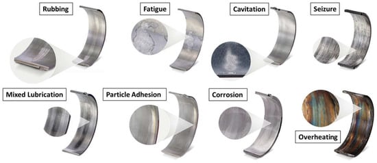
Figure 1.
Damage mechanisms commonly found in journal bearings.
2.1. Mixed Elastohydrodynamic Lubrication Model
The governing equations of the mixed elastohydrodynamic lubrication model for a plain journal bearing utilized in this work are briefly presented below. Figure 2 illustrates the main geometric and kinematic parameters of the model. This section summarizes previous publications where a more detailed explanation of the numerical procedure is included, and the reader is referred to references [44,45,46].
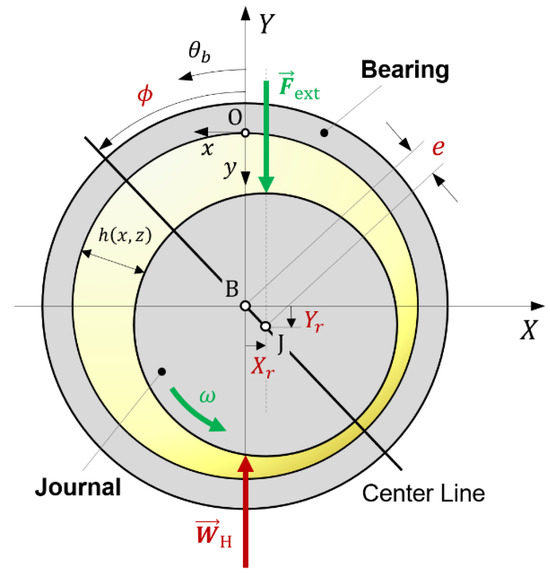
Figure 2.
Schematic of the journal bearing model with the main geometrical and kinematic parameters.
2.1.1. Reynolds Equation
The hydrodynamic pressure developed within the lubricant film at the journal bearing interface is calculated using the steady-state isothermal Reynolds equation with the Elrod–Adams p–θ mass-conserving cavitation model, which can be written as
with the complementarity conditions for cavitation being as follows:
2.1.2. Film Thickness Equation
In this work, any misalignment between the crankshaft pin and the connecting rod is neglected. Consequently, the lubricant film thickness can be expressed in the local coordinate system as
2.1.3. Elastic Deformation Equation
The bearing flexibility must be incorporated into the model to account for surface deformations induced by the fluid pressure under elastohydrodynamic (EHD) conditions. Since only surface elastic displacements are relevant for fluid pressure calculations in the EHD regime, finite element substructuring (also referred to as superelement or condensed modelling techniques) [47] is applied to reduce the full structural finite element model of the bearing system to an equivalent model containing only the degrees of freedom associated with the nodes located on the bearing surface. In this study, the reduced FEM model of the bearing system, including both the structural dynamics and distributed inertia, is expressed as
2.1.4. Rheological Models
The rheological behaviour of a lubricant significantly influences the lubrication performance of ICE connecting rod bearings. The rheological properties of lubricants are highly dependent on the temperature, pressure, and shear rate. Since an isothermal steady-state lubrication condition is assumed in this work, only the corrections for the density–pressure, viscosity–pressure (or piezoviscous), and viscosity–thinning relationships are considered. The viscosity–pressure relationship is modelled using the isothermal Barus equation [48] in Equation (5):
Sliding bearings are prone to generating high shear rates within the lubricant film, especially in high-speed engines. Under these conditions, the assumption of Newtonian fluid behaviour is no longer valid, as the lubricant can exhibit shear thinning characteristics. In fully formulated engine oils, polymer-based viscosity modifier additives can contribute to the shear thinning effect, thereby influencing the lubricant viscosity at moderate and high shear rates. In this study, the power law-based Carreau–Yasuda equation was employed to calculate the lubricant viscosity decrease due to shear thinning behaviour [49].
These viscosity corrections are carried out using a partitioned coupling method with the respective shear rate and hydrodynamic pressure calculations to obtain the final viscosity value when the iterative process converges. A more detailed explanation can be found in [44].
Regarding the density–pressure correction, the well-known Dowson–Higginson equation is used [50], formulated in Equation (7):
2.1.5. Asperity Contact Model
Tribological interactions at the microscale have been studied using different approaches in the literature. The statistical [51,52,53,54] and deterministic [55,56,57] methods are the most notable in this field. These methods can be considered for implementation in the current fluid–structure interaction (FSI) framework. The method selected for this work was the statistical-based Greenwood and Tripp model for rough contacts due to its wide use in tribology simulations. Furthermore, this contact model incorporates the elastoplastic behaviour of the materials. When the asperity contact pressure, calculated using the Greenwood–Tripp equation, exceeds the hardness of the softer material in the coupling, the asperity contact pressure is limited to the hardness of that softer material. The complete formulation is presented in Equation (8):
The combined roughness parameters are calculated as mentioned in [51]. However, the combined asperity density and mean radius of the curvature are calculated following the approach in [58], where a more specific method is proposed to achieve better contact area prediction.
2.1.6. Load Balance and Friction Equations
Journal bearings are subjected to different load scenarios. The steady-state loading conditions are considered in this work using the following equilibrium equation (see Figure 2).
where is the resulting combined hydrodynamic and contact forces and is the externally applied load. The combined force components represented in the vector basis as the axes of the coordinates system BXYZ attached to the bearing centre are calculated by integrating the fluid and asperity contact pressure fields over the bearing domain, as shown in Equation (10):
Furthermore, the frictional force produced by the viscous interaction of the fluid with the moving surfaces and asperity interactions between the journal and bearing surfaces, the latter computed considering Coulomb–Amontons’ law for dry solid contacts, is calculated using Equation (11):
where is the hydrodynamic shear stress and is the effective fluid viscosity, which depends on whether the fluid is flowing within the pressurized () or cavitation () regions, and it is defined by the weighting function determining the local changes in the dynamic viscosity as a function of the fluid film fraction distribution . In cavitation regions (), is equivalent to the viscosity of the homogeneous mixture of the liquid and vapour lubricant; in pressurized regions (), equals the viscosity of the liquid lubricant.
2.2. Proposed Wear Model
Calculating the wear on lubricated sliding surfaces is complex due to various influencing parameters like the sliding speed, contact area, pressure, lubricant, and surface roughness. This work introduces a novel wear algorithm that defines specific time steps based on six criteria, incorporates a nonlocal averaging function from contact mechanics, and uses a multiscale roughness model to adjust the roughness in wear regions. The algorithm targets applications with frequent asperity contacts, such as those in internal combustion engines (ICEs), industrial machines, turbines, and electric motors. It integrates a mixed elastohydrodynamic lubrication model for lubrication and contact mechanics predictions within a custom MATLAB toolbox LUBST. Figure 3 illustrates the simulation workflow, from the input variables to result processing and wear cycle updates.
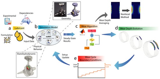
Figure 3.
Wear algorithm scheme: (a) lubricant input data; (b) simulation framework for mixed elastohydrodynamic lubrication; (c) wear algorithm used to predict wear; (d) wear evolution over time; (e) wear cycle boundary conditions.
The algorithm begins with setting up the simulation model by inputting parameters such as the lubricant and geometry characteristics, bearing stiffness, roughness, boundary conditions, and bearing speed and load. The boundary conditions are updated in each iteration, where the wear model computes the time step and wear based on tribological interactions from the mixed EHL simulation. Various wear prediction models utilize empirical and numerical methods, often relying on data for the sliding speed, temperature, load, and material properties. This work employs Archard’s model to predict the local wear depth, integrating a new formulation [59] to factor in the energy required for material removal during stable wear. Key variables include the hardness of the softer material H, the wear intensity constant K, the local friction power per area , and the contact duration ∆t. The final equation for the wear depth is then calculated at each computational mesh node:
A brief explanation of the wear load and time step highlights the dependence of the variables included in Archard’s equation for wear depth prediction. The new proposed approach assumes that the material removal rate remains constant during a certain period, (the time step). This enables the consideration in the model of the average wear load during this period, which represents the local rate of the friction energy loss per area. The average wear load is defined in Equation (13) and depends on the asperity contact pressure , the relative velocity between the surfaces , and the shaft rotation period under stable wear conditions.
An appropriate time step in the wear prediction algorithm is crucial for obtaining accurate results and is defined by six criteria, as shown in Figure 4. A large time step can result in divergences or incorrect wear regions. The first criterion initiates the process after 100 revolutions at a specified speed and resets the process if the speed changes or divergences occur. The second criterion relates to the wear depth predicted by Archard’s equation, limiting increments to 0.5 µm per node to prevent an excessive wear concentration. The third criterion, which is independent of the asperity pressure, doubles the previous time step if the wear predictions are below the maximum limit. The fourth criterion adjusts the time step based on the previous asperity pressures to stabilize convergence: it retains or doubles the step based on whether the pressure is below 1 MPa, above 5 MPa, or in between. The fifth criterion aims to prevent divergencies by reverting to the previous time step if the current asperity pressure is more than double the previous one or resetting if it is four times greater. Lastly, the sixth criterion terminates the iterative process when no wear conditions are present, choosing the remaining time as the current time step.
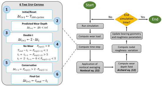
Figure 4.
Wear algorithm flowchart.
In the wear algorithm, once the time step and wear load field are established, the wear depth is computed at each node of the bearing shell. This updates the value for the film thickness between the bearing and journal surfaces and is followed by the recalculation of the hydrodynamic and asperity contact pressures for the worn geometry. However, mesh resolution issues can lead to inaccurate local contact pressure predictions. To address these inaccuracies and convergence problems, a nonlocal method for determining contact mechanics is proposed. This method incorporates a multiscale roughness model to account for roughness variations in the wear regions, ensuring an accurate prediction of the material removal at each node.
2.2.1. Nonlocal Function Based on Contact Mechanics
Spatial discretization is a technique in numerical modelling where a finite number of points, or nodes, represent a continuum system. Common methods include the finite element method (FEM) and Boundary Elements Method (BEM). However, these methods can lead to issues due to information loss from discretizing a continuum, particularly in predicting tribological interactions. This can result in unrealistic local overshoots in variables like the contact pressures. Nonlocal methods can address these problems by avoiding unrealistic local concentrations and are utilized in various fields, including the prediction of crack propagation in damage mechanics.
Different specific averaging functions of nonlocal methods can be used with different approaches: integral or differential types. In this study, the integral type was used, and its implementation involves substituting the computed wear load at each node with an averaged value according to the following expression:
where is computed by
The wear load at every node is evaluated according to this expression, where is the nonlocal wear load and is the local value. As indicated in Equation (14), the averaging procedure is driven by the nonlocal weight function , whose value decreases with the distance to the evaluated point . Therefore, a specific radius of influence is considered to affect the neighbourhood of a particular node, and all neighbouring nodes are assigned a ratio indicated by the weight function. This work proposes a more specific treatment of the radius of action as the function of a local variable related to the rough contact mechanics behaviour of the bearing. The variable selected was the asperity shear stress, defined as the asperity pressure times the boundary coefficient of friction . This variable was made dimensionless to ensure a manageable range using the Hertz shear stress as the reference value characteristic of the material. Accordingly,
Regarding the radius of action (Ra), an ellipse shape was chosen to represent the shape of the neighbouring area for sliding wear conditions. The largest axis of the ellipse is parallel to the sliding direction and is defined as the radius of action in Equation (17); the shortest axis is defined as a function of the specific ellipse eccentricity of 0.6 selected as shown in Equation (19). For ease of understanding, the common abbreviations for the ellipse semi-radius, and , are used in the equations. In Equation (17), denotes the limits of the neighbouring area, but in the equations any mesh has a different aspect ratio and node-to-node distance.
A specific definition for each one is proposed to correctly align the maximum and minimum radius with those in the case study. depends on the geometry configuration of the bearing based on the number of topography samples in the circumferential direction times the bearing clearance, as shown in Equation (18).
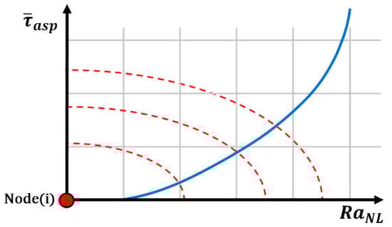
Figure 5.
Radius of action function for nonlocal contact mechanics.
Furthermore, a new weight function is proposed to account for the variation in the local ellipse radius (R) as a function of the local position of the neighbour node with respect to the reference node and the angle and the local value of . The local R variation is shown in Equation (20). The local variation in the area of influence is selected based on the specific conditions of the sliding bearings. The proposed weight function is expressed in Equation (21). In this equation, is the distance to the neighbour node from the reference node.
The final expression of the nonlocal wear load is shown in Equation (22), where the boundary treatment is included for the nodes near the edges of the lubricated domain. The value of refers to the value of far from the boundaries.
A graphical illustration of the nonlocal method is depicted in Figure 6 to enhance understanding. An example of the connecting rod bearing is shown in detail without any result preprocessing, where the wear load contours are shown over the bearing mesh. The influence area is represented by a red line forming the local ellipse shape, where the wear load is distributed in the neighbouring nodes coloured in black with a Gaussian weighting function. To ensure a correct distribution, the area was adjusted to the bearing edges based on the limit, as indicated in Equation (22).
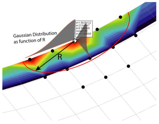
Figure 6.
Nonlocal contact mechanics scheme.
2.2.2. Multiscale Roughness Evolution Model
Wear is a process in which material is removed from a surface, and this can be predicted using numerical methods. However, wear predictions are sensitive to the spatial discretization of the lubricated domain. The predicted wear depth at computational mesh nodes can vary with the resolution of the mesh, while actual wear occurs at the microscale, influenced by the surface roughness. This disparity may lead to overestimations of the hydrodynamic pressures and friction losses because there is often a disconnect between the macro-level wear predictions and microscale surface topography.
To address this issue, the authors propose a method to link the material removal across scales. Each macro node corresponds to a specific area of influence for the wear, and an equivalent microscale topography is adjusted to reflect the predicted material loss. This correlation utilizes a multiscale parameter, the wear volume per area, connected via the volume distribution by height curve, known as the Abbott curve [60].
Visualizing this requires the use of Probability Density Functions (PDFs) to illustrate the roughness height distribution. From the PDF, a Cumulative Density Function (CDF) is derived, representing the surface height-to-material ratio. The material area ratio can then be converted to a volume ratio, ensuring uniformity in the topography mesh. The Abbott curve is represented as 1 − the CDF to depict the material removal at specific heights, effectively bridging the gap between the predicted macro wear and actual microscale topography, as shown in Figure 7.
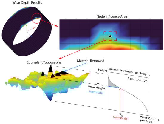
Figure 7.
Multiscale roughness evolution model scheme.
Surface characterization is critical to obtain the roughness parameters at different wear stages. A method developed by the authors [61] is to obtain specific Greenwood–Tripp [51] roughness parameters from every surface topography (see Figure 8), where the asperity pressure is calculated using a statistical approach that accounts for the asperity density, the asperity peak radius of the curvature, the standard deviation of the asperity height, the contact area, the composite elastic modulus, the surface separation, and the integral function related to the asperity height distribution (see Section 2.1.5).
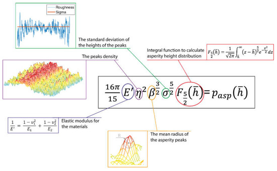
Figure 8.
Greenwood–Tripp equation illustration.
Every surface exhibits unique roughness parameters, determined at the microscale, which can undergo alterations due to various phenomena such as deformation, wear, and melting. It is imperative to calculate pertinent variables to accurately characterize these roughness features, as no universally accepted methodology exists for their acquisition. Hence, in this study, we employed a proprietary algorithm to identify asperity peaks based on a specified percentage of the root mean square (RMS) height of the surface’s three-dimensional (3D) topography. This process enabled the detection of the primary peaks in the measurement, which were the initial contact points with another surface. Subsequently, the density of the asperity peaks was computed as the ratio of the number of peaks to the total surface area. Furthermore, the standard deviation of the peak heights was determined. Utilizing the identified peaks as reference points, the mean radius of the curvature of the asperity peaks was calculated by examining four directions: parallel, perpendicular, and along two diagonals to the neighbouring nodes. The median of these four radii yielded the parameter representing the characteristic curvature of the peaks.
2.3. Mixed EHL and Wear Model Coupling
This section describes the complete iterative algorithm setup and numerical solution procedure for the steady-state, isothermal, elastic plain journal bearing system comprising wear and multiscale roughness models. The flowchart depicted in Figure 9 illustrates the procedure carried out during a simulation. The steady-state solution for the mixed EHL model was obtained by solving the nonlinear equilibrium equations for the relative rigid body displacements of the journal with respect to the bearing. To solve these nonlinear equations and obtain the EHL solution, the Newton–Raphson (NR) method and Point Gauss–Seidel Method with Aitken Acceleration (PGMA) were employed, utilizing Armijo’s linear search technique to optimize the solution step size at each iteration. Within the framework of the Newton–Raphson iterative process, the Reynolds equation was numerically solved using the hybrid Element-Based Finite Volume Method (EBVM) as proposed by Profito [44,45], specifically designed for lubrication problems encompassing mass-conserving cavitation on unstructured meshes. The Gauss–Seidel method with Successive Over-Relaxation (SOR) was employed to solve the discretized Reynolds equation. The details about the hydrodynamic mesh will be shown in the following sections. The numerical parameters of the solver settings are shown in Table 1.
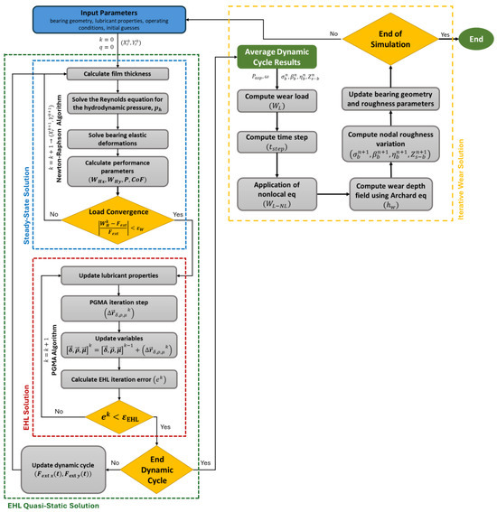
Figure 9.
M-EHL and wear algorithm coupling scheme.

Table 1.
Numerical settings for the simulations.
Furthermore, a convergence study was conducted to determine the most suitable mesh configuration. Various grid sizes were simulated to compare the results for the hydrodynamic meshes of the journal bearing. Since the mesh was regular and each element was a square, different side lengths were chosen for the simulations: 1 mm (2550 nodes), 1.5 mm (1212 nodes), and 2 mm (696 nodes). The results of this study indicated negligible variation in the hydrodynamic variables among these grid sizes; however, significant differences were observed in the predicted wear area due to a smaller contact patch associated with the larger grid sizes. Consequently, a smaller grid size was selected to better represent a more continuous contact area.
After reaching the steady-state and EHL solutions, the process of obtaining the iterative wear solution started immediately, as this case study was set up with a static load and the external forces did not evolve over time. The wear algorithm calculated the corresponding wear load and time step and applied the nonlocal function to the wear load field. Then, the wear depth field was computed using Archard’s equation, and the multiscale roughness model was used to calculate the variation in the Greenwood–Tripp roughness parameters at the microscale based on the wear depth predicted at the macroscale. Once these subroutines were finished, the bearing geometry, roughness parameters, and operating conditions were updated in the next iterative cycle.
3. Case Study
The case study focused on an experimental bearing test rig that assessed journal bearing wear depth profiles under a static load, constant shaft speed, and constant oil temperature. This scenario allowed us to effectively validate the wear model due to the clear data and reproducibility it provided [62,63,64]. Figure 10 shows the experimental rig for the connecting rod bearing.
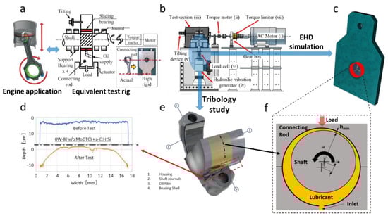
Figure 10.
Case study illustration: (a) real engine application and test rig selected; (b) detailed scheme of test rig; (c) connecting rod finite element model; (d) experimental measurement of bearing axial profiles, before and after wear cycle; (e) interaction of parts selected for tribology study; (f) lubrication scheme of connection rod journal bearing.
The test machine consisted of an electric motor driving a shaft with a torque transducer to measure the friction losses. The test bearing was mounted on a rigid connecting rod and statically loaded by a hydraulic actuator, with support brackets and bearings. The journal bearing received oil at 4 MPa and 110 °C into the unloaded shell. The key geometrical parameters for the simulation model are detailed in Table 2.
Table 2.
Test rig specifications.
The roughness parameters were obtained using the method from the multiscale roughness evolution model, essential for predicting the asperity contact pressure in the Greenwood–Tripp equation and for friction and wear assessments. For accurate tribological predictions, 3D surface measurements were necessary. The bearing surface characterization setup is illustrated in Figure 11, while Figure 12 depicts the surface evolution and the vectorization of the roughness parameters used during operation to minimize the computation costs.
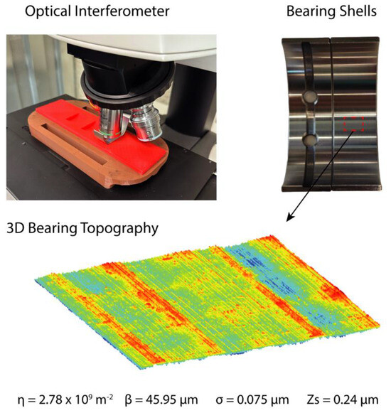
Figure 11.
Topography characterization of bearing surface.
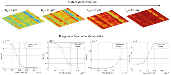
Figure 12.
Surface roughness parameters’ evolution with wear.
It is important to notice that the bearing surface studied was highly smooth. Therefore, the roughness parameters did not vary drastically because the lower limit of the surface was reached with a few micrometres of wear.
3.1. Simulation Model
This study developed a new simulation model to virtualize the connecting rod bearing test rig from [62,63,64], aiming to predict the lubrication conditions under various operational parameters (rotational speed, load, temperature, lubricant type). The core of this model is the FEM representation of the connecting rod bearing, accounting for its elastic deformation under load, which is crucial for accurate lubrication performance predictions in wear conditions. This deformation relates to the hydrodynamic and asperity contact pressures, creating a fluid–structure interaction (FSI) problem. The hydrodynamic mesh was tailored to the bearing’s characteristics, with oil supplied through a 180-degree groove in the top shell, as illustrated in Figure 13, and its spatial discretization is detailed in Table 2.
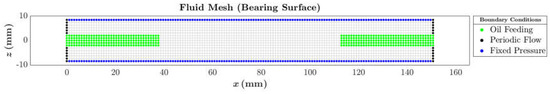
Figure 13.
Hydrodynamic mesh scheme.
The FEM model used in the simulation is shown in Figure 10c, with its parameters detailed in Table 3. An iterative mesh independence study ensured reliable results. The full connecting rod model was simplified to focus on the inner cylindrical surface of the bearing shell, reducing the computational costs while maintaining accuracy. To optimize efficiency, C3D8 elements were used for the stiffness matrix and CQUAD4 elements served as intermediaries between the bearing and fluid domains. Only the CQUAD4 elements were loaded in the simulation, incorporating the necessary mass and stiffness properties of the bearing components.
Table 3.
Hydrodynamic and FEM meshes’ specifications.
3.2. Lubricant Candidates
This study evaluated the wear characteristics of three ultralow-viscosity lubricant formulations: Oil A, Oil B, and Oil C. Each formulation combined synthetic base stocks with a variety of additives, including viscosity modifiers, friction modifiers, antioxidants, corrosion inhibitors, detergents, anti-wear agents, anti-foam additives, nanoparticles, and dispersants, as referenced in [42,65,66]. A reference lubricant (Ref 0W-8) [67] was also used for benchmarking against the bearing wear.
Table 4 outlines the compositions of the lubricants, highlighting the predominance of synthetic base stocks and the equal proportion of additives across all formulations. These lubricants were developed and characterized at the Repsol Technology Lab in Mostoles, Madrid, Spain.
Table 4.
Repsol lubricants’ composition.
Table 5 outlines the properties of the lubricants tested for wear protection at 110 °C, revealing the key differences among them. Oil A displayed Newtonian behaviour with a constant viscosity, while Oils B and C showed shear thinning behaviour typical of non-Newtonian fluids, as per the Carreau model [69]. The lubricants’ heat transfer properties were also crucial due to thermal generation during contact, affecting the film temperature. The average oil temperatures were stabilized during the wear cycle, allowing for isothermal simulations that disregarded transient fluctuations. Additionally, with high loads, the lubricant film pressure could exceed 200 MPa, reinforcing the need for the Barus model [48] to describe the dynamic viscosity’s pressure dependence, as detailed in Table 4.
Table 5.
Repsol lubricants’ properties.
In tribology, various factors affect the outcomes due to the interactions between rough surfaces. The boundary coefficient of friction (CoF) is crucial for simulating the behaviour of lubricants in mixed lubrication conditions, necessitating the use of tribometers that can replicate thin oil film environments. The mini traction machine (MTM) tribometer at the Repsol Technology Lab was utilized to gather data across varying shear rates, temperatures, and loads, as presented in previous work [38,39,70].
To accurately reflect the journal bearing conditions in the MTM, an equivalence study focused on the contact pressure was conducted. Hertz’s theory helped link the MTM point contacts to the journal bearing line contacts, providing the necessary contact pressure for the simulation. The resulting friction maps, created under different conditions, enabled the determination of the average CoF for the lubricants under mixed and boundary lubrication conditions. For further information regarding these procedures, please consult reference [70].
In this study, the average CoF values were used for the oils, with a standard CoF of 0.2 applied under critical wear conditions, representing dry contact and facilitating calculations of the asperity tangential shear stress.
3.3. Wear Cycle Procedure
To study transient sliding wear in journal bearings, dynamic simulations were conducted with a constant shaft speed and oil temperature, varying the static load. The wear cycle derived from [62,63,64] includes two phases: the first at 5200 rpm and 3 kN and the second with a load ranging from 3 kN to 99 kN. This work focused solely on the second phase to analyze the wear conditions, as the first phase serves as a stabilization period. The simulation employed experimental boundary conditions, including an average oil temperature of 110 °C and a supply pressure of 4 bar, as shown in Figure 14. These conditions were ideal for validating the wear model and calibrating the Archard wear intensity parameter against the experimental wear rates.
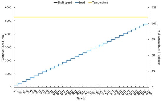
Figure 14.
Wear cycle illustration.
4. Results and Discussion
This section provides a detailed evaluation of the results obtained for the three engine lubricants. Initially, the results of a wear validation are presented to ensure that the wear rate and maximum wear depth values are consistent with those reported in the reference study. Subsequently, the analysis is divided into subsections that focus on the dependence of key factors, including the nonlocal function, the multiscale roughness evolution model, and the wear behaviour of ultralow-viscosity lubricants.
4.1. Wear Validation
This study used experimental data from Refs. [62,63,64] to validate the amount of material removed from the bearing shell. The oil used for this validation was an SAE 0W-8 oil from [67] due to the limited oil data published by the authors and the references available for similar lubricants. The scenario selected in which to validate the simulation model involved a DLC-coated journal and AlSnZn alloy bearing, which were tested during a wear cycle with a constant speed of 5200 rpm, a constant load increased in steps of 120 s from 3 kN to 99 kN, an isothermal condition of 110 °C, and a total duration of 3960 s.
The authors characterized the roughness of the journal bearing surfaces with an optical interferometer for a purchased sample of the bearing shells used in the reference articles [62,63,64], as shown in Figure 11. Journal shaft roughness data from the references were insufficient to feed the Greenwood–Tripp model; therefore, data from a similar study with a DLC-coated engine part was used [71], where the topography of a valvetrain shaft was characterized, and the following Greenwood–Tripp roughness parameters were obtained: σ = 0.165 μm, η = 4.5 × 10¹¹ 1/m2, β = 1.17 μm, and Zs = 0.47 μm.
The complexity of the wear validation process was caused by various factors, such as the experimental uncertainty, local boundary conditions, physical behaviour of materials during the wear process, and the directional seizure area of the bearing, among others. Therefore, to simplify the process, an axial profile of the maximum wear depth was measured using a linear roughness machine, as described in Ref. [62]. The results obtained using the simulation model were compared with the experimental measurements at macroscale dimensions. Figure 15 compares the wear profiles at the end of the wear cycle for the bottom bearing shell, indicated by a dashed red line in the image of the bearing shell used in the study. The results in the figure demonstrate good agreement between the experimental and simulated profiles, verifying the predictive capability of the simulation model.
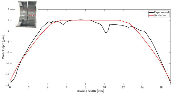
Figure 15.
Wear depth validation.
4.2. Multiscale Roughness Evolution Model Assessment
This subsection describes the evaluation of the local evolution of the surface roughness as a function of the lubricant used. The multiscale roughness evolution model was used in all cases, with the vectorized surface roughness parameters being a function of the wear depth. This approach enabled the assessment of boundary conditions under which the surface roughness might evolve differently. The evolution of the asperity pressure with the dimensionless oil film thickness is depicted in Figure 16 to show the importance of varying the roughness parameters. This curve shows the output of the Greenwood–Tripp equation.
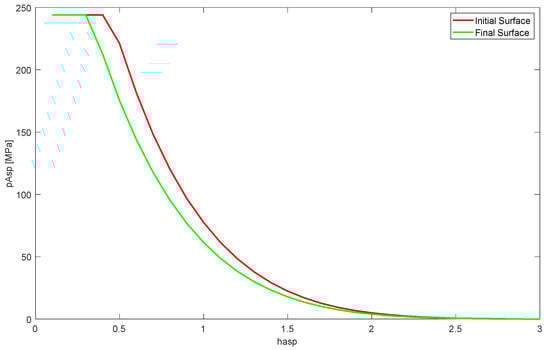
Figure 16.
Dependence of asperity pressure on dimensionless film thickness and surface roughness.
The values for the asperity pressure tended to decrease as the surface was subjected to wear. This case study used smooth surfaces for the bearing and journal. However, the variation in the roughness within wear regions caused a significant change in the contact pressure calculated using the Greenwood–Tripp equation. This variation became more relevant with an increasing magnitude of the studied surface’s roughness.
The most relevant roughness parameter variations in the bearing shells are plotted in Figure 17 to enhance the understanding of the local topography evolution.
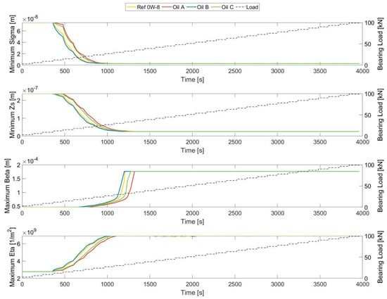
Figure 17.
Roughness parameters’ evolution over the wear cycle.
Figure 17 shows the evolution of the maximum asperity peak density, minimum mean asperity height, minimum mean square root of the asperity height, and maximum mean asperity radius, the roughness parameters used to calculate the surface contact conditions. The method proposed by the authors assumes the dependence of the roughness characteristics is a function of the wear on the bearing shell. The lubricants demonstrated different tendencies as their wear rates differed significantly. Oil A showed lower variation in its roughness parameters, while Oil C, Ref 0W-8, and Oil B were the candidates with more variation during the first loading steps. However, the bearing surface in this study was smooth, and the wear conditions were severe, reaching around 10 microns of wear depth. The lubricants ultimately converged to the same values for all the surface roughness parameters. Video S1 is included in the Supplementary Material to enhance the understanding of the evolution of the local roughness parameters.
4.3. Wear Assessment with Ultralow-Viscosity Lubricants
Different ultralow-viscosity lubricant formulations were assessed regarding their wear protection capabilities as a complementary objective of this study. The steady-state conditions of the wear cycle were highly demanding in terms of the lubricant’s performance due to the need to maintain its viscosity with an increasing temperature and shear rate and create a lubricant film under high loads. Such conditions are found in high-power-density engines, where the performance is maximized to deliver the maximum output power. Lubricants play a crucial role in engine durability, as their protective film thickness prevents excessive wear in reciprocating and rotational mechanisms.
Therefore, a wear assessment procedure is presented by which we compared the lubricants’ performance based on previous publications [38,39]. This procedure was structured according to several key elements: a representative scenario of the actual application, a validated simulation model to ensure correct wear prediction, and a wear algorithm with time step prediction as a function of the change in the wear rate that ensured convergence. Thus, the following results are presented to comprehensively assess the wear protection capabilities of ultralow-viscosity lubricants in high-performance engines.
A comparison of the evolution of the lubrication conditions over the wear cycle is presented with the corresponding instantaneous power loss to enhance the understanding of wear assessment. Lubrication regimes help us to understand when critical wear conditions are occurring and can be calculated using the specific oil film thickness (SOFT) . Following a literature review [20], the lubrication regimes according to the SOFT values were classified as follows: <1: boundary, when critical damage occurs due to severe surface contact; 1–3: mixed, where surface contact often causes damage; 3–4: elastohydrodynamic, a regime associated with elastic deformation and some possible surface contacts; and >4: hydrodynamic, a regime in which there is no contact, as there is significant separation between surfaces.
Figure 18 shows the evolution of the minimum SOFT values over the wear cycle considered. Significant material removal in some areas of the bearing was observed. In the first cycle, the minimum SOFT values revealed that the bearing was still in the hydrodynamic regime, but it quickly changed to the mixed lubrication regime due to the load increase. At around 3000 s, all lubricants performed according to a boundary lubrication regime due to the highly loaded conditions. As a general tendency observed in the graph, Oil A showed a high SOFT value, which means a better wear protection capability. It was closely followed by Oil C, which showed similar wear protection capabilities. The use of Ref 0W-8 oil generally resulted in lower SOFT values, coming in third overall. Oil B yielded the lowest SOFT values, showing the worst wear protection capabilities following the assessment based on the lubrication regime results.
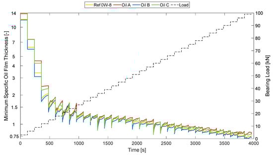
Figure 18.
Evolution of minimum SOFT values over the wear cycle.
Another interesting result from the assessment of lubricant performance under friction power loss is depicted in Figure 19, which shows how much energy was expended due to tribological and rheological losses. Lubricant additives determine these results, as well as the level of wear protection. Therefore, the correct combination of additives must achieve a good compromise between the friction losses and wear protection. In this case, Oil B exhibited higher values for friction losses, showing worse performance in terms of energy efficiency. It was followed by Ref 0W-8 and Oil C, respectively. Oil A showed the lowest friction loss values, indicating that this oil was the best selection for this loading condition.
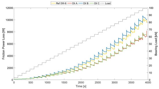
Figure 19.
Friction power loss evolution over the wear cycle.
In addition, the wear intensity and the total amount of material removed observed during the simulations were analyzed, and several results are provided below. So, the wear intensity was measured based on the wear load and asperity pressure values. The main difference between these two variables was the nonlocal function applied to the wear load results to obtain an averaged solution following the contact mechanics approach. However, the tendencies of these two variables matched and agreed with the previous assumptions based on the SOFT results. Figure 20, showing the wear load and asperity pressure results, depicts the same performance hierarchy as for the friction power loss, with Oil B exhibiting the highest wear intensity values, followed by Ref 0W-8 and Oil C; Oil A was the lubricant with the lowest wear intensity values. Video S1 is included in the Supplementary Material to enhance the understanding of the evolution of the local contact conditions.
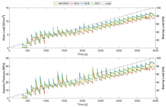
Figure 20.
Wear load and asperity pressure evolution over the wear cycle.
Regarding the amount of material removed from the bearing, Figure 21 shows the results obtained for the four lubricants. Both the maximum wear depth and wear volume are shown in the figure, with significant differences in their evolution over time but not in the lubricants’ final results. The maximum wear depth showed a tendency to increase smoothly over the wear cycle, with Oil B being the lubricant with the least protective capabilities, followed by Ref 0W-8 and Oil C, respectively. The results for Oil A agreed with those from the previous assessment, showing the lowest wear depth values.
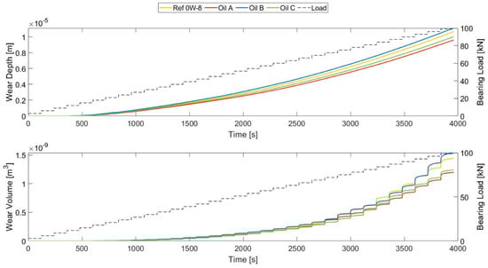
Figure 21.
Accumulated wear depth and wear volume evolution over the wear cycle.
However, different tendencies were observed for the wear volume over the wear cycle, where the lubricants did not maintain the same performance hierarchy at all points. This phenomenon can be explained by the equilibrium in the contact area when a significant amount of material was removed quickly from a region, such as the bearing’s edges. Then, the inner regions tended to compensate for this excessive wear at the edges. Therefore, the wear volume tended to evolve according to the maximum wear depth at the end of the cycle when the contact areas had stabilized. Thus, the performance hierarchy of the lubricants matched the results for the maximum wear depth values.
Lastly, wear depth contours are shown in Figure 22 as the final results to enhance the visualization of the damage caused to the bearing shells and for the lubricant wear assessment. The results from the last time step for the wear depth are depicted for the four lubricants in Figure 22. The contour plots show the influence of the connecting rod’s elasticity, which caused the wear areas to shift to the bearing’s edges due to a high amount of deformation in the centre region caused by the high hydrodynamic pressure.
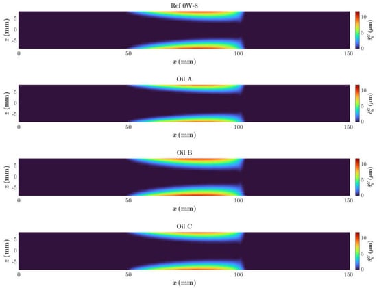
Figure 22.
Wear depth contours at the final time step of the wear cycle.
An axial cross section is shown for the maximum wear depth region in Figure 23 at x = 81 mm to facilitate a comparison between the lubricants. It can be seen that the results matched those of the previous assessment, with the order from the lowest wear protection capabilities to the most being Oil B, Ref 0W-8, Oil C, and Oil A. It was confirmed that Oil A showed better durability capabilities in this case study in terms of its wear protection and power loss efficiency.
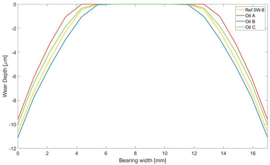
Figure 23.
Wear depth axial profile at x = 81 mm at the final time step of the wear cycle.
5. Conclusions
The novel algorithm proposed in this work for predicting wear on the connecting rod bearings of internal combustion engines has demonstrated high effectiveness and reliability. By incorporating multiple factors, including the sliding speed, contact area, hydrodynamic and asperity contact pressures, lubricant properties, and surface roughness evolution, the algorithm provides a comprehensive and robust framework suitable for making wear predictions in complex tribological systems. The integration of a nonlocal averaging function, specifically designed to account for the contact mechanics characteristics of the interface, significantly enhanced the accuracy of the wear distribution calculations by mitigating unrealistic local asperity contact concentrations associated with the resolution of the computational mesh.
This work also emphasizes the importance of dynamically adjusting the surface roughness parameters during wear simulations. The proposed multiscale roughness evolution model provided a deeper understanding of how the surface roughness evolves under varying lubrication conditions, particularly with different lubricants. The validations against experimental data revealed strong agreement in terms of the wear rates and maximum wear depths, confirming the model’s reliability in practical applications.
Additionally, this study highlighted significant performance differences among low-viscosity lubricants, identifying specific lubricants that provide superior wear protection and energy efficiency. Such findings make these lubricants more suitable for high-demand applications. Overall, this contribution offers significant insights into the design and optimization of tribological systems, particularly in high-performance engines and industrial machinery.
While this study provides valuable insights into the performance analysis of fully formulated lubricants using a virtual test bench, certain limitations are acknowledged. The translation of MTM-derived friction coefficients to the full complexity of real-world operational conditions, including dynamic surface changes, presents inherent challenges despite the existence of measures like the contact pressure equivalence. Furthermore, the assessment of commercial lubricants which vary in terms of their base oil, additives, and viscosity simultaneously makes isolating the specific contribution of individual parameters to the performance outcomes more complex. Therefore, while incorporating the detailed experimental characterization of lubricants, the numerical model used in this work focused on macroscopic rheological and tribological properties rather than explicitly simulating the microscale chemical interactions of specific lubricant components.
Supplementary Materials
The following supporting information can be downloaded at https://www.mdpi.com/article/10.3390/lubricants13050230/s1: Video S1: Wear cycle video.
Author Contributions
Conceptualization, J.B.-R., J.P. and F.J.P.; methodology, J.B.-R.; formal analysis, J.B.-R. and F.J.P.; resources, M.C.-G.; writing—original draft preparation, J.B.-R.; writing—review and editing, J.B.-R., J.P., M.C.-G. and F.J.P.; visualization, J.B.-R.; supervision, J.P., M.C.-G. and F.J.P. All authors have read and agreed to the published version of the manuscript.
Funding
This research received no external funding.
Data Availability Statement
The data that support the findings of this study are available from the corresponding authors upon reasonable request.
Acknowledgments
We would like to express our gratitude to our partners from Repsol SA, which financed this research and contributed to the development of new lubricant formulations using simulation tools, and we would also like to express our gratitude to all our colleagues from CINTECX who contributed to the success of this research.
Conflicts of Interest
Author Marti Cortada-Garcia was employed by Repsol SA. The remaining authors declare that the research was conducted in the absence of any commercial or financial relationships that could be construed as a potential conflict of interest.
Nomenclature
| Lubricant density | |
| Lubricant film thickness | |
| Lubricant’s dynamic viscosity | |
| Local coordinate system | |
| Hydrodynamic pressure | |
| Rotational speed | |
| Saturation pressure | |
| Lubricant film fraction | |
| R | Nominal bearing radius |
| Circumferential direction | |
| Axial direction | |
| Pressured regions | |
| Cavitation regions | |
| Cavitation boundaries | |
| Coordinate system in the bearing centre | |
| Rigid body displacements of the journal relative to the bearing in the BX direction | |
| Rigid body displacements of the journal relative to the bearing in the BY direction | |
| Bearing clearance | |
| Angular position of the bearing | |
| Elastic deformations of the bearing surface in the radial direction | |
| Elastic deformations of the journal surface in the radial direction | |
| Reduced mass matrix | |
| Reduced damping matrix | |
| Reduced stiffness matrix | |
| Nodal surface displacement vector in the local bearing coordinate system | |
| Nodal surface velocity vector in the local bearing coordinate system | |
| Nodal surface acceleration vector in the local bearing coordinate system | |
| Nodal hydrodynamic pressure vector | |
| Area matrix used to convert the fluid pressure into a distributed load field on the bearing surface | |
| Low-shear Newtonian dynamic viscosity at a given temperature and pressure | |
| Barus constant (specific to each lubricant) | |
| Carreau–Yasuda constants (specific to each lubricant) | |
| Characteristic relaxation time of the lubricant | |
| Equivalent shear rate within the fluid film | |
| Lubricant’s dynamic viscosity at infinite shear rate | |
| , | Dowson–Higginson constants with typical values of 0.59 GPa and 1.34 |
| Lubricant density at atmospheric pressure and given temperature | |
| Rough contact pressure | |
| Specific oil film thickness (SOFT) | |
| Combined elastic modulus of the surface materials | |
| Vickers’ hardness of the softer material | |
| Combined asperity density | |
| Combined asperity radius of curvature | |
| Standard deviation of the asperity heights | |
| Mean asperity height | |
| Gaussian function representing the asperity height distributions approximated by a polynomial function [51] | |
| Combined hydrodynamic and contact forces | |
| Externally applied load | |
| Hydrodynamic shear stress | |
| Asperity shear stress | |
| Weighting function for local changes in the dynamic viscosity | |
| Effective fluid viscosity | |
| Wear depth | |
| Wear time step | |
| Local friction power per area (or wear load) | |
| Wear intensity constant | |
| Hardness of the softer surface material | |
| Relative velocity between surfaces | |
| Shaft rotation period | |
| Nonlocal wear load | |
| Nonlocal weight function | |
| Distance to the evaluated point | |
| Ra | Radius of action |
| Boundary coefficient of friction | |
| Hertz shear stress | |
| Ultimate shear stress | |
| Ultimate tensile stress | |
| Ellipse eccentricity | |
| , | Ellipse long and short semi-radius |
| Limits of the neighbouring area | |
| Bearing radius | |
| Number of topography samples in circumferential direction | |
| Dimensionless asperity shear stress | |
| Local ellipse radius | |
| θ | Local angle variation with respect to a reference node |
| Limit of the value far from the boundaries |
References
- Ramalho, A.; Miranda, J.C. The Relationship between Wear and Dissipated Energy in Sliding Systems. Wear 2006, 260, 361–367. [Google Scholar] [CrossRef]
- Ramalho, A. A Reliability Model for Friction and Wear Experimental Data. Wear 2010, 269, 213–223. [Google Scholar] [CrossRef]
- Maier, M.; Pusterhofer, M.; Grün, F. Modelling Approaches of Wear-Based Surface Development and Their Experimental Validation. Lubricants 2022, 10, 335. [Google Scholar] [CrossRef]
- Machado, T.H.; Cavalca, K.L. Investigation on an Experimental Approach to Evaluate a Wear Model for Hydrodynamic Cylindrical Bearings. Appl. Math. Model. 2016, 40, 9546–9564. [Google Scholar] [CrossRef]
- Zhang, S.; Hao, Q.; Liu, Y.; Jin, L.; Ma, F.; Sha, Z.; Yang, D. Simulation Study on Friction and Wear Law of Brake Pad in High-Power Disc Brake. Math. Probl. Eng. 2019, 2019. [Google Scholar] [CrossRef]
- Yang, Y.; Ling, L.; Wang, J.; Zhai, W. A Numerical Study on Tread Wear and Fatigue Damage of Railway Wheels Subjected to Anti-Slip Control. Friction 2023, 11, 1470–1492. [Google Scholar] [CrossRef]
- Lehmann, B.; Trompetter, P.; Guzmán, F.G.; Jacobs, G. Evaluation of Wear Models for the Wear Calculation of Journal Bearings for Planetary Gears in Wind Turbines. Lubricants 2023, 11, 364. [Google Scholar] [CrossRef]
- Archard, J.F. Contact and Rubbing of Flat Surfaces. J. Appl. Phys. 1953, 24, 981–988. [Google Scholar] [CrossRef]
- Ireman, P.; Klarbring, A.; Strömberg, N. Finite Element Algorithms for Thermoelastic Wear Problems. Eur. J. Mech.—A/Solids 2002, 21, 423–440. [Google Scholar] [CrossRef]
- Beheshti, A.; Khonsari, M.M. An Engineering Approach for the Prediction of Wear in Mixed Lubricated Contacts. Wear 2013, 308, 121–131. [Google Scholar] [CrossRef]
- Bartel, D.; Bobach, L.; Illner, T.; Deters, L. Simulating Transient Wear Characteristics of Journal Bearings Subjected to Mixed Friction. Proc. Inst. Mech. Eng. Part J J. Eng. Tribol. 2012, 226, 1095–1108. [Google Scholar] [CrossRef]
- Kalogiannis, K.; Merritt, D.R.; Mian, O.; Morina, A.; Neville, A.; Liskiewicz, T. Contact and Wear Thermo-Elastohydrodynamic Model Validation for Engine Bearings. Proc. Inst. Mech. Eng. Part J J. Eng. Tribol. 2017, 231, 1117–1127. [Google Scholar] [CrossRef]
- Pijaudier-Cabot, G.; Bažant, Z.P. NonLocal Damage Theory. J. Eng. Mech. 1987, 113. [Google Scholar] [CrossRef]
- Jirásek, M. Nonlocal Damage Mechanics. Rev. Eur. De Génie Civ. 2007, 11, 993–1021. [Google Scholar] [CrossRef]
- Shaat, M.; Ghavanloo, E.; Fazelzadeh, S.A. Review on Nonlocal Continuum Mechanics: Physics, Material Applicability, and Mathematics. Mech. Mater. 2020, 150, 103587. [Google Scholar] [CrossRef]
- Giry, C.; Dufour, F.; Mazars, J. Stress-Based Nonlocal Damage Model. Int. J. Solids Struct. 2011, 48, 3431–3443. [Google Scholar] [CrossRef]
- Bažant, Z.P.; Pijaudier-Cabot, G. Nonlocal Continuum Damage, Localization Instability and Convergence. J. Appl. Mech. Trans. ASME 1988, 55, 287–293. [Google Scholar] [CrossRef]
- Bažant, Z.P.; Pijaudier-Cabot, G. Measurement of Characteristic Length of Nonlocal Continuum. J. Eng. Mech. 1989, 115, 755–767. [Google Scholar] [CrossRef]
- Kennedy, T.C.; Nahan, M.F. A Simple NonLocal Damage Model for Predicting Failure of Notched Laminates. Compos. Struct. 1995, 35, 229–236. [Google Scholar] [CrossRef][Green Version]
- Burstein, L. Lubrication and Roughness. In Tribology for Engineers; Woodhead Publishing: Delhi, India, 2011. [Google Scholar]
- Morales-Espejel, G.E.; Brizmer, V.; Piras, E. Roughness Evolution in Mixed Lubrication Condition Due to Mild Wear. Proc. Inst. Mech. Eng. Part. J J. Eng. Tribol. 2015, 229, 1330–1346. [Google Scholar] [CrossRef]
- Galera, L.; De, A.; Rodrigues, S.; Malburg, M.C. Importance of Connecting Rod and Crankshaft Roughness Accuracy on Sliding Bearing Performance. SAE Tech. Pap. 2015. [Google Scholar] [CrossRef]
- Hanief, M.; Wani, M.F. Modeling and Prediction of Surface Roughness for Running-in Wear Using Gauss-Newton Algorithm and ANN. Appl. Surf. Sci. 2015, 357, 1573–1577. [Google Scholar] [CrossRef]
- Qiu, M.; Chen, L.; Li, Y.; Yan, J. Bearing Tribology Principles and Applications; Springer: Berlin/Heidelberg, Germany, 2015. [Google Scholar]
- Vladescu, S.C.; Marx, N.; Fernández, L.; Barceló, F.; Spikes, H. Hydrodynamic Friction of Viscosity-Modified Oils in a Journal Bearing Machine. Tribol. Lett. 2018, 66, 127. [Google Scholar] [CrossRef]
- Santos, N.D.S.A.; Roso, V.R.; Faria, M.T.C. Review of Engine Journal Bearing Tribology in Start-Stop Applications. Eng. Fail. Anal. 2020, 108, 104344. [Google Scholar] [CrossRef]
- Summer, F.; Bergmann, P.; Grün, F. Damage Equivalent Test Methodologies as Design Elements for Journal Bearing Systems. Lubricants 2017, 5, 47. [Google Scholar] [CrossRef]
- Taylor, R.I. Rough Surface Contact Modelling—A Review. Lubricants 2022, 10, 98. [Google Scholar] [CrossRef]
- Xu, G.; Sadeghi, F. Thermal EHL Analysis of Circular Contacts With Measured Surface Roughness. J. Tribol. 1996, 118, 473–482. [Google Scholar] [CrossRef]
- Morales-Espejel, G.E. Surface Roughness Effects in Elastohydrodynamic Lubrication: A Review with Contributions. Proc. Inst. Mech. Eng. Part J J. Eng. Tribol. 2014, 228, 1217–1242. [Google Scholar] [CrossRef]
- Ai, X.; Cheng, H.S. A Transient EHL Analysis for Line Contacts With Measured Surface Roughness Using Multigrid Technique. J. Tribol. 1994, 116, 549–556. [Google Scholar] [CrossRef]
- Sadeghi, F.; Sui, P.C. Compressible Elastohydrodynamic Lubrication of Rough Surfaces. J. Tribol. 1989, 111, 56–62. [Google Scholar] [CrossRef]
- MAHLE GmbH. Pistons and Engine Testing, 2nd ed.; ATZ/MTZ-Fachbuch; Springer: Stuttgart, Germany, 2016. [Google Scholar]
- Nicolò Mastrandrea, L.; Giacopini, M.; Dini, D.; Bertocchi, E. Elastohydrodynamic Analysis of the Conrod Small-End of A High Performance Motorbike Engine via A Mass Conserving Cavitation Algorithm. In Proceedings of the ASME 2015 International Mechanical Engineering Congress and Exposition IMECE2015, Houston, TX, USA, 13–19 November 2015; ASME: Houston, TX, USA, 2015. [Google Scholar]
- Kalogiannis, K.; Desai, P.; Mian, O.; Mainwaring, R. Simulated Bearing Durability and Friction Reduction with Ultra-Low Viscosity Oils. SAE Tech. Pap. 2018. [Google Scholar] [CrossRef]
- Honda R&D Co., Ltd. Honda R&D Technical Review F1 Special (The 3rd Era Activities); Honda Motor Co., Ltd.: Tokyo, Japan, 2009. [Google Scholar]
- Boretti, A. Engine Design Concepts for World Championship Grand Prix Motorcycles; SAE International: Warrendale, PA, USA, 2012. [Google Scholar]
- Blanco-Rodríguez, J.; Porteiro, J.; López-Campos, J.A.; Domínguez, B.; Cortada-Garcia, M. Friction Assessment of Ultralow Viscosity Lubricant Formulations Based on a Validated Elastohydrodynamic Simulation. Int. J. Engine Res. 2023, 24, 146808742311621. [Google Scholar] [CrossRef]
- Blanco-Rodríguez, J.; Porteiro, J.; López-Campos, J.A.; Cortada-García, M.; Fernández-Castejón, S. Wear Protection Assessment of Ultralow Viscosity Lubricants in High-Power-Density Engines: A Novel Wear Prediction Algorithm. Friction 2024, 12, 1785–1800. [Google Scholar] [CrossRef]
- Vakis, A.I.; Yastrebov, V.A.; Scheibert, J.; Nicola, L.; Dini, D.; Minfray, C.; Almqvist, A.; Paggi, M.; Lee, S.; Limbert, G.; et al. Modeling and Simulation in Tribology across Scales: An Overview. Tribol. Int. 2018, 125, 169–199. [Google Scholar] [CrossRef]
- Meng, Y.; Xu, J.; Jin, Z.; Prakash, B.; Hu, Y. A Review of Recent Advances in Tribology. Friction 2020, 8, 221–300. [Google Scholar] [CrossRef]
- Meng, Y.; Xu, J.; Ma, L.; Jin, Z.; Prakash, B.; Ma, T.; Wang, W. A Review of Advances in Tribology in 2020–2021. Friction 2022, 10, 1443–1595. [Google Scholar] [CrossRef]
- Rahnejat, H. Tribology and Dynamics of Engine and Powertrain; Woodhead Publishing Limited: Sawston, UK, 2010. [Google Scholar]
- Profito, F.J.; Zachariadis, D.C.; Dini, D. Partitioned Fluid-Structure Interaction Techniques Applied to the Mixed-Elastohydrodynamic Solution of Dynamically Loaded Connecting-Rod Big-End Bearings. Tribol. Int. 2019, 140, 105767. [Google Scholar] [CrossRef]
- Profito, F.J.; Zachariadis, D.C. Partitioned Fluid-Structure Methods Applied to the Solution of Elastohydrodynamic Conformal Contacts. Tribol. Int. 2015, 81, 321–332. [Google Scholar] [CrossRef]
- Profito, F.J.; Giacopini, M.; Zachariadis, D.C.; Dini, D. A General Finite Volume Method for the Solution of the Reynolds Lubrication Equation with a Mass-Conserving Cavitation Model. Tribol. Lett. 2015, 60, 18. [Google Scholar] [CrossRef]
- Zienkiewicz, O.C.; Taylor, R.L.; Zhu, J.Z. The Finite Element Method: Its Basis and Fundamentals Sixth Edition, 6th ed.; Elsevier: Amsterdam, The Netherlands, 2005. [Google Scholar]
- Barus, C. Isothermals, Isopiestics and Isometrics Relative to Viscosity. Am. J. Sci. 1890, s3-45, 87–96. [Google Scholar] [CrossRef]
- Kazunori, Y. A Multi-Mode Viscosity Model and Its Applicability to Non-Newtonian Fluids. J. Text. Eng. 2006, 52, 171–173. [Google Scholar]
- Dowson, D.; Higginson, G.R. Elasto-Hydrodynamic Lubrication; Pergamon Press: Oxford, UK, 1977. [Google Scholar]
- Greenwood, J.A.; Tripp, J.H. The Contact of Two Nominally Flat Rough Surfaces. Proc. Instn. Mech. Engrs. 1970, 625–633. [Google Scholar] [CrossRef]
- Greenwood, J.A.; Williamson, J.B.P. Contact of Nominally Flat Surfaces. Proc. R. Soc. Lond. A Math. Phys. Sci. 1966, 295, 300–319. [Google Scholar] [CrossRef]
- Bush, A.W.; Gibson, R.D.; Thomas, T.R. The Elastic Contact of A Rough Surface; Elsevier Sequoia S.A.: Amsterdam, The Netherlands, 1975; Volume 35. [Google Scholar]
- Kogut, L.; Etsion, I. A Finite Element Based Elastic-Plastic Model for the Contact of Rough Surfaces. Tribol. Trans. 2003, 46, 383–390. [Google Scholar] [CrossRef]
- Wang, Z.J.; Wang, W.Z.; Hu, Y.Z.; Wang, H. A Numerical Elastic-Plastic Contact Model for Rough Surfaces. Tribol. Trans. 2010, 53, 224–238. [Google Scholar] [CrossRef]
- Medina, S.; Dini, D. A Numerical Model for the Deterministic Analysis of Adhesive Rough Contacts down to the Nano-Scale. Int. J. Solids Struct. 2014, 51, 2620–2632. [Google Scholar] [CrossRef]
- Keer, L.M.I.A. Polonsky Fast Methods for Solving Rough Contact Problems: A Comparative Study. 2000. Available online: http://asmedigitalcollection.asme.org/tribology/article-pdf/122/1/36/5820179/36_1.pdf (accessed on 20 September 2024).
- Beheshti, A.; Khonsari, M.M. Asperity Micro-Contact Models as Applied to the Deformation of Rough Line Contact. Tribol. Int. 2012, 52, 61–74. [Google Scholar] [CrossRef]
- Sander, D.E.; Allmaier, H.; Priebsch, H.H.; Reich, F.M.; Witt, M.; Skiadas, A.; Knaus, O. Edge Loading and Running-in Wear in Dynamically Loaded Journal Bearings. Tribol. Int. 2015, 92, 395–403. [Google Scholar] [CrossRef]
- Bigerelle, M.; Iost, A.; Bigerelle, M.; Iost, A. A Numerical Method to Calculate the Abbott Parameters: A Wear Application. Tribol. Int. 2007, 40, 1319–1334. [Google Scholar] [CrossRef]
- García-Rodiño, D.; Blanco-Rodríguez, J.; Cortada-García, M.; Fernández, S.; Porteiro, J. A Numerical Procedure for Calculating Roughness Parameters for the Greenwood Tripp Model of Asperity Contact Based on 3D Measurements. Tribol. Int. 2024, 200, 110156. [Google Scholar] [CrossRef]
- Ogihara, H.; Mihara, Y.; Kano, M. Seizure and Friction Properties of the DLC Coated Journal and Aluminum Alloy Bearing. Tribol. Online 2020, 15, 241–250. [Google Scholar] [CrossRef]
- Iwata, T.; Oikawa, M.; Chida, R.; Ishii, D.; Ogihara, H.; Mihara, Y.; Kano, M. Excellent Seizure and Friction Properties Achieved with a Combination of an A-c:H:Si Dlc-Coated Journal and an Aluminum Alloy Plain Bearing. Coatings 2021, 11, 1055. [Google Scholar] [CrossRef]
- Ogihara, H.; Iwata, T.; Mihara, Y.; Kano, M. The Effects of DLC-Coated Journal on Improving Seizure Limit and Reducing Friction under Engine Oil Lubrication. Int. J. Engine Res. 2022, 23, 1267–1274. [Google Scholar] [CrossRef]
- Spikes, H. Friction Modifier Additives. Tribol. Lett. 2015, 60, 5. [Google Scholar] [CrossRef]
- Zhao, J.; Huang, Y.; He, Y.; Shi, Y. Nanolubricant Additives: A Review. Friction 2021, 9, 891–917. [Google Scholar] [CrossRef]
- Yamamori, K.; Uematsu, Y.; Manabe, K.; Miyata, I.; Kusuhara, S.; Misaki, Y. Development of Ultra Low Viscosity 0W-8 Engine Oil. SAE Tech. Pap. 2020. [Google Scholar] [CrossRef]
- American Petroleum Institute. Engine Oil Licensing and Certification System; American Petroleum Institute: Washington, DC, USA, 2021. [Google Scholar]
- Carreau, P.J. Rheological Equations from Molecular Network Theories. Trans. Soc. Rheol. 1972, 16, 99–127. [Google Scholar] [CrossRef]
- Blanco-Rodríguez, J. On the Development of a Comprehensive Damage Prediction Algorithm for Mixed-Elastohydrodynamic Lubrication Conditions in High-Power Density Engines. Ph.D. Thesis, Universidade de Vigo, Vigo, Spain, 2025. [Google Scholar] [CrossRef]
- Lyu, B.; Meng, X.; Zhang, R.; Cui, Y. A Comprehensive Numerical Study on Friction Reduction and Wear Resistance by Surface Coating on Cam/Tappet Pairs under Different Conditions. Coatings 2020, 10, 485. [Google Scholar] [CrossRef]


Disclaimer/Publisher’s Note: The statements, opinions and data contained in all publications are solely those of the individual author(s) and contributor(s) and not of MDPI and/or the editor(s). MDPI and/or the editor(s) disclaim responsibility for any injury to people or property resulting from any ideas, methods, instructions or products referred to in the content. |
© 2025 by the authors. Licensee MDPI, Basel, Switzerland. This article is an open access article distributed under the terms and conditions of the Creative Commons Attribution (CC BY) license (https://creativecommons.org/licenses/by/4.0/).