Complex Working Condition Bearing Fault Diagnosis Based on Multi-Feature Fusion and Improved Weighted Balance Distribution Adaptive Approach


Abstract
1. Introduction
2. Methodology
2.1. Signal Denoising
2.2. Feature Extraction
2.2.1. Frequency Features
2.2.2. Distribution Entropy and Its Variants
2.2.3. Refined Composite Multivariate Generalized Multiscale Fuzzy Entropy
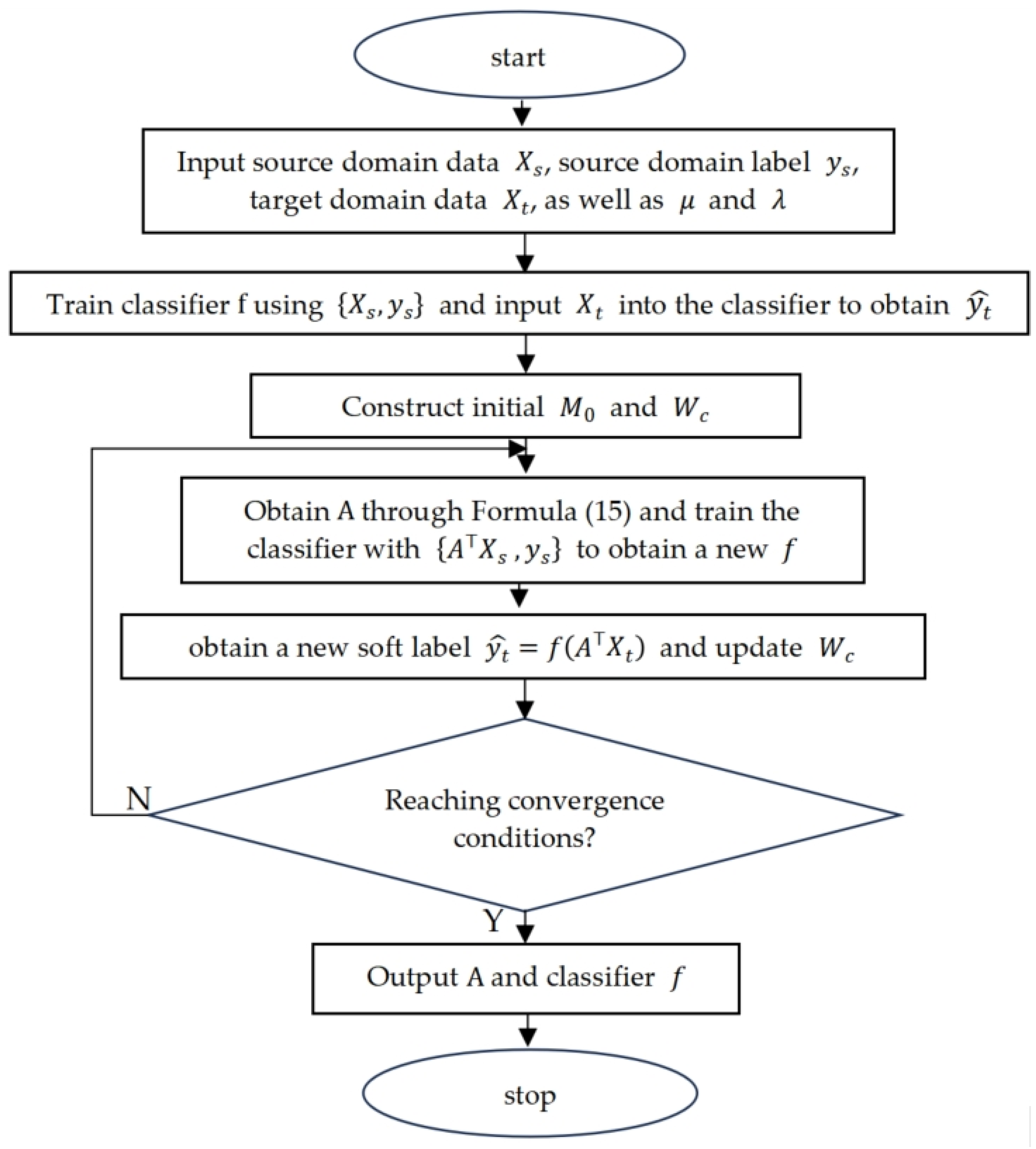
2.3. WBDA Feature Transfer
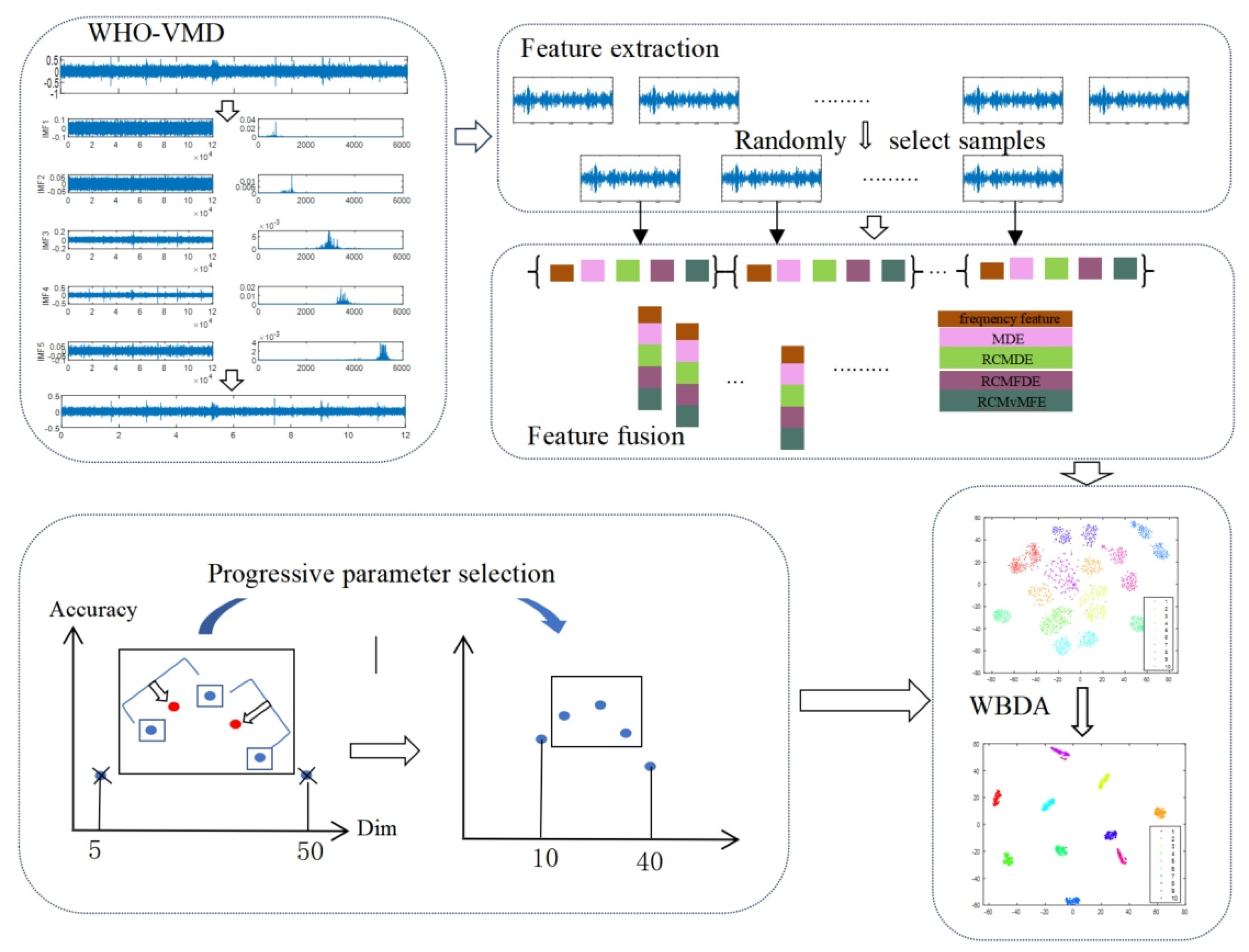
3. The MFF-IWBDA Model
4. Experimental Analyses
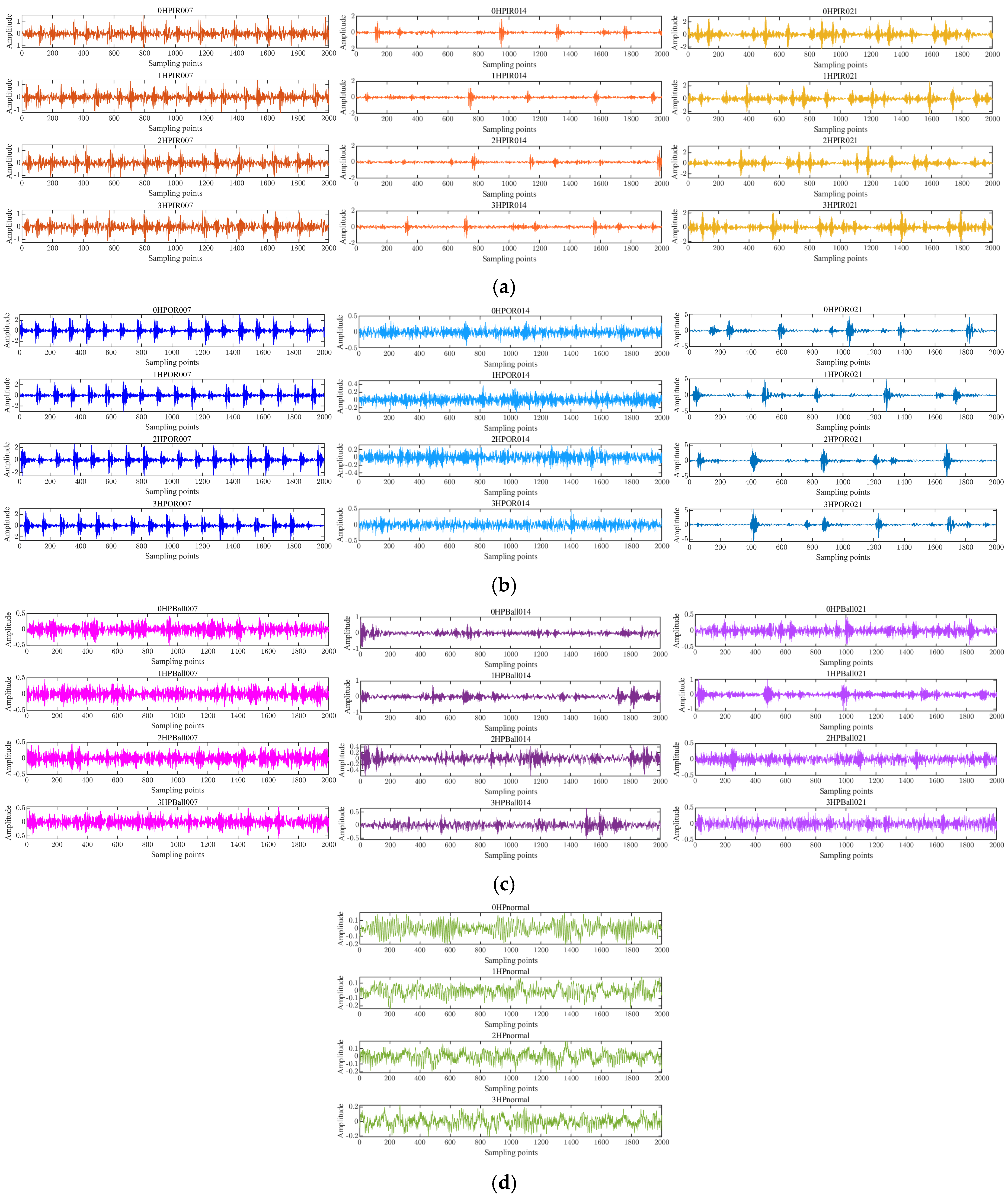
4.1. The Dataset Description
4.2. Analysis of Experimental Results
4.3. Feature Extraction and Fusion Analysis
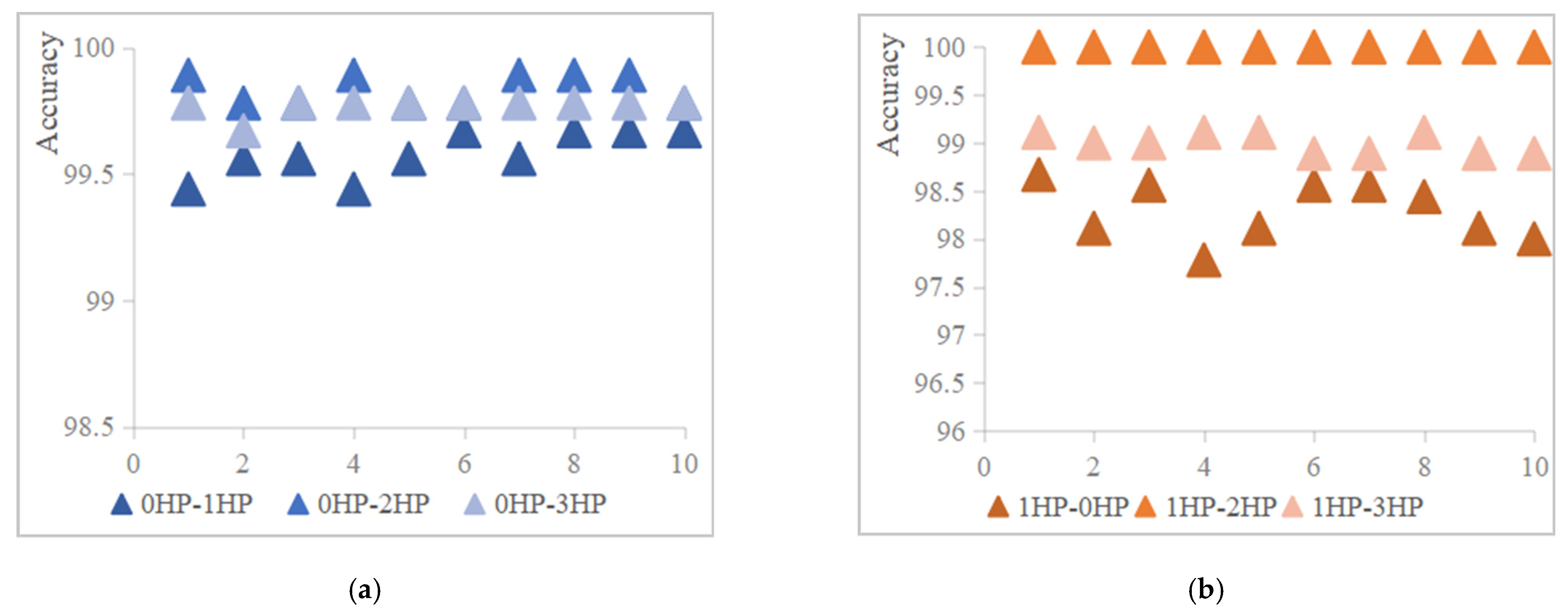
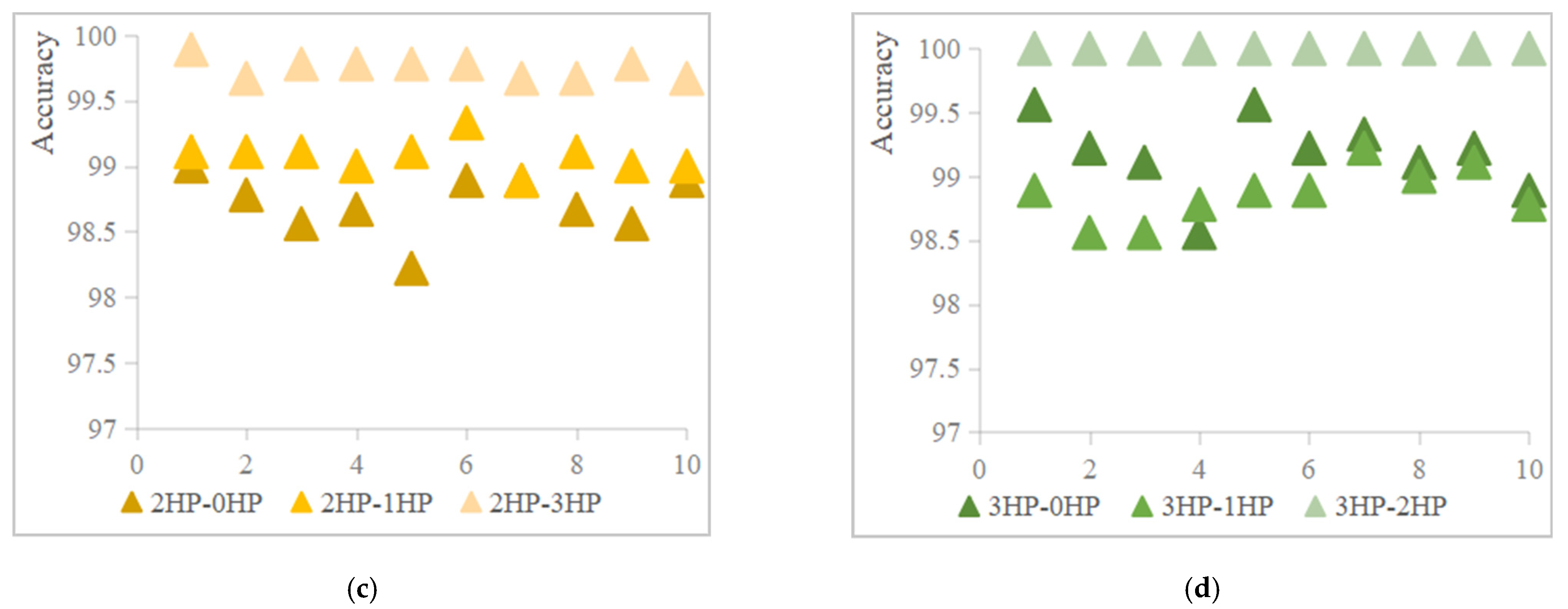
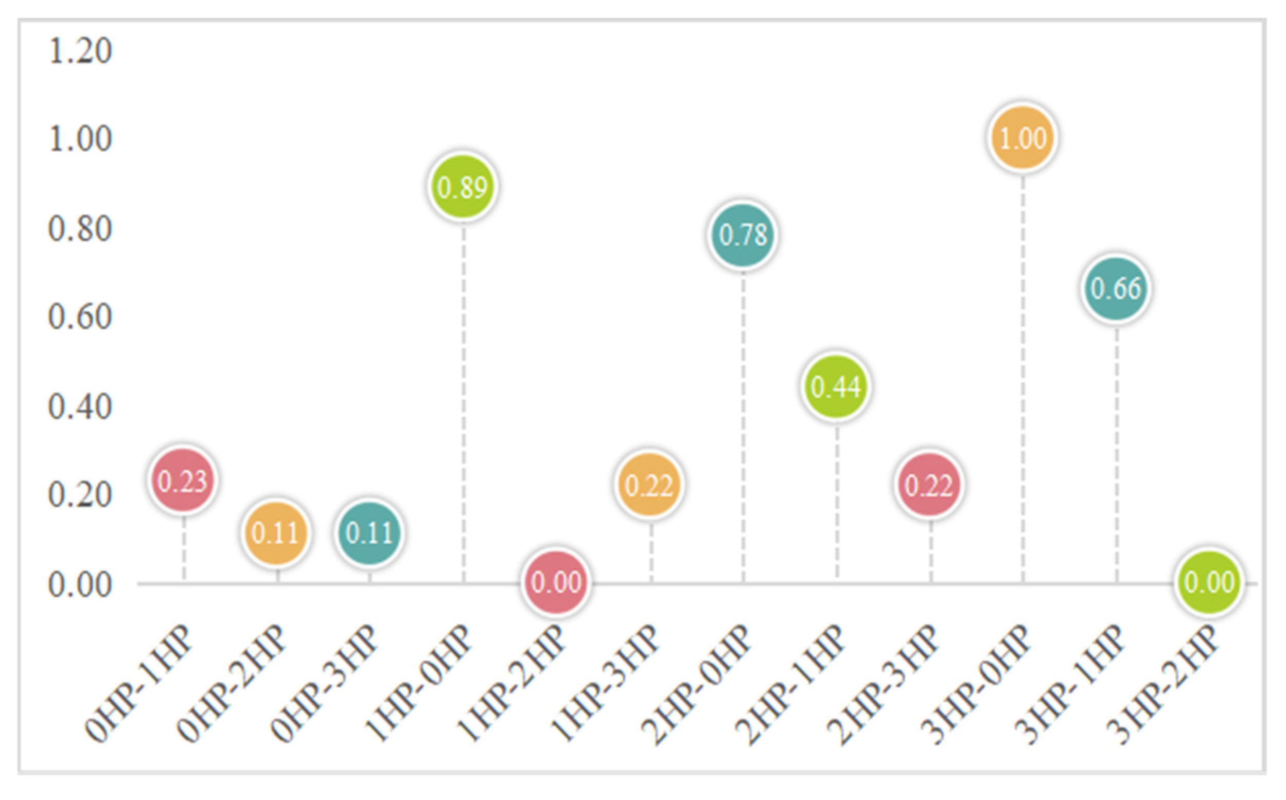
4.4. Model Stability Analysis
4.5. Comparison of Transfer Models
4.6. Comparative Analysis of Models
5. Conclusions
Author Contributions
Funding
Data Availability Statement
Acknowledgments
Conflicts of Interest
References
- Dong, X.; Zhang, C.; Liu, H.; Wang, D.; Chen, Y.; Wang, T. A new cross-domain bearing fault diagnosis method with few samples under different working conditions. J. Manuf. Process. 2025, 135, 359–374. [Google Scholar] [CrossRef]
- He, D.; Wu, J.; Jin, Z.; Huang, C.G.; Wei, Z.; Yi, C. AGFCN: A bearing fault diagnosis method for high-speed train bogie under complex working conditions. Reliab. Eng. Syst. Saf. 2025, 258, 110907. [Google Scholar] [CrossRef]
- Tahir, M.M.; Khan, A.Q.; Iqbal, N.; Iqbal, N.; Hussain, A.; Badshah, S. Enhancing fault classification accuracy of ball bearing using central tendency based time domain features. IEEE Access 2016, 5, 72–83. [Google Scholar] [CrossRef]
- Junior, R.F.R.; dos Santos Areias, I.A.; Gomes, G.F. Fault detection and diagnosis using vibration signal analysis in frequency domain for electric motors considering different real fault types. Sens. Rev. 2021, 41, 311–319. [Google Scholar] [CrossRef]
- Ruiz-Sarrio, J.E.; Antonino-Daviu, J.A.; Martis, C. Comprehensive Diagnosis of Localized Rolling Bearing Faults during Rotating Machine Start-Up via Vibration Envelope Analysis. Electronics 2024, 13, 375. [Google Scholar] [CrossRef]
- Zheng, J.; Huang, S.; Pan, H.; Tong, J.; Wang, C.; Liu, Q. Adaptive power spectrum Fourier decomposition method with application in fault diagnosis for rolling bearing. Measurement 2021, 183, 109837. [Google Scholar] [CrossRef]
- Shao, H.; Lin, J.; Zhang, L.; Wei, M. Compound fault diagnosis for a rolling bearing using adaptive DTCWPT with higher order spectral. Qual. Eng. 2020, 32, 342–353. [Google Scholar] [CrossRef]
- Hao, Y.; Zhang, C.; Lu, Y.; Zhang, L.; Lei, Z.; Li, Z. A novel autoencoder modeling method for intelligent assessment of bearing health based on Short-Time Fourier Transform and ensemble strategy. Precis. Eng. 2024, 85, 89–101. [Google Scholar] [CrossRef]
- Liang, P.; Tian, J.; Wang, S.Y.X. Multi-source information joint transfer diagnosis for rolling bearing with unknown faults via wavelet transform and an improved domain adaptation network. Reliab. Eng. Syst. Saf. 2024, 242, 109788. [Google Scholar] [CrossRef]
- Wang, W.; Yuan, H. Bearing Fault Feature Extraction Method Based on Adaptive Time-Varying Filtering Empirical Mode Decomposition and Singular Value Decomposition Denoising. Machines 2025, 13, 50. [Google Scholar] [CrossRef]
- Tu, Z.; Gao, L.; Wu, X.; Liu, Y.; Zhao, Z. Rotate vector reducer fault diagnosis model based on EEMD-MPA-KELM. Appl. Sci. 2023, 13, 4476. [Google Scholar] [CrossRef]
- Yan, J.; Zhou, F.; Zhu, X.; Zhang, D. AFSA-FastICA-CEEMD Rolling Bearing Fault Diagnosis Method Based on Acoustic Signals. Mathematics 2025, 13, 884. [Google Scholar] [CrossRef]
- Dai, X.; Yi, K.; Wang, F.; Cai, C.; Tang, W. Bearing fault diagnosis based on POA-VMD with GADF-Swin Transformer transfer learning network. Measurement 2024, 238, 115328. [Google Scholar] [CrossRef]
- Shen, J.; Wang, Z.; Wang, Y.; Zhu, H.; Zhang, L.; Tang, Y. AGWO-PSO-VMD-TEFCG-AlexNet bearing fault diagnosis method under strong noise. Measurement 2025, 242, 116259. [Google Scholar] [CrossRef]
- Li, H.; Wu, X.; Liu, T.; Li, S.; Zhang, B.; Zhou, G.; Huang, T. Composite fault diagnosis for rolling bearing based on parameter-optimized VMD. Measurement 2022, 201, 111637. [Google Scholar] [CrossRef]
- Qiu, W.; Wang, B.; Hu, X. Rolling bearing fault diagnosis based on RQA with STD and WOA-SVM. Heliyon 2024, 10, e26141. [Google Scholar] [CrossRef]
- Gao, L.; Wang, X.; Wang, T.; Chang, M. WDBM: Weighted deep forest model based bearing fault diagnosis method. Comput. Mater. Contin. 2022, 72, 4742–4754. [Google Scholar] [CrossRef]
- Quan, Z.; Zhang, X. Rolling bearing fault diagnosis based on CS-optimized multiscale dispersion entropy and ML-KNN. J. Braz. Soc. Mech. Sci. Eng. 2022, 44, 430. [Google Scholar]
- Song, X.; Wang, H.; Liu, Y.; Wang, Z.; Cui, Y. A fault diagnosis method of rolling element bearing based on improved PSO and BP neural network. J. Intell. Fuzzy Syst. 2022, 43, 5965–5971. [Google Scholar] [CrossRef]
- Yu, J.; Ding, B.; He, Y. Rolling bearing fault diagnosis based on mean multigranulation decision-theoretic rough set and non-naive Bayesian classifier. J. Mech. Sci. Technol. 2018, 32, 5201–5211. [Google Scholar] [CrossRef]
- Yuan, L.; Lian, D.; Kang, X.; Chen, Y.; Zhai, K. Rolling bearing fault diagnosis based on convolutional neural network and support vector machine. IEEE Access 2020, 8, 137395–137406. [Google Scholar] [CrossRef]
- Tang, S.; Wang, C.; Zhou, F.; Hu, X.; Wang, T. Multi-scale recursive semi-supervised deep learning fault diagnosis method with attention gate. Machines 2023, 11, 153. [Google Scholar] [CrossRef]
- Zhou, C.; Wang, Q.; Xiao, Y.; Xiao, W.; Shu, Y. Research on an Improved Auxiliary Classifier Wasserstein Generative Adversarial Network with Gradient Penalty Fault Diagnosis Method for Tilting Pad Bearing of Rotating Equipment. Lubricants 2023, 11, 423. [Google Scholar] [CrossRef]
- Wang, B.; Liang, P.; Zhang, L.; Wang, X.; Yuan, X.; Zhou, Z. Enhancing robustness of cross-machine fault diagnosis via an improved domain adversarial neural network and self-adversarial training. Measurement 2025, 250, 117113. [Google Scholar] [CrossRef]
- Deng, C.; Tian, H.; Miao, J.; Deng, Z. Domain adaptation method based on pseudo-label dual-constraint targeted decoupling network for cross-machine fault diagnosis. Reliab. Eng. Syst. Saf. 2025, 256, 110786. [Google Scholar] [CrossRef]
- He, D.; Lao, Z.; Jin, Z.; He, C.; Shan, S.; Miao, J. Train bearing fault diagnosis based on multi-sensor data fusion and dual-scale residual network. Nonlinear Dyn. 2023, 111, 14901–14924. [Google Scholar] [CrossRef]
- He, C.; He, D.; Wei, Z.; Xu, K.; Chen, Y.; Shan, S. A train bearing imbalanced fault diagnosis method based on extended CCR and multi-scale feature fusion network. Nonlinear Dyn. 2024, 112, 13147–13173. [Google Scholar] [CrossRef]
- Wang, X.; Li, A.; Han, G. A deep-learning-based fault diagnosis method of industrial bearings using multi-source information. Appl. Sci. 2023, 13, 933. [Google Scholar] [CrossRef]
- Wu, M.; Zhang, J.; Xu, P.; Liang, Y.; Dai, Y.; Gao, T.; Bai, Y. Bearing Fault Diagnosis for Cross-Condition Scenarios Under Data Scarcity Based on Transformer Transfer Learning Network. Electronics 2025, 14, 515. [Google Scholar] [CrossRef]
- Dragomiretskiy, K.; Zosso, D. Variational Mode Decomposition. IEEE Trans. Signal Process. 2014, 62, 531–544. [Google Scholar] [CrossRef]
- Naruei, I.; Keynia, F. Wild horse optimizer: A new meta-heuristic algorithm for solving engineering optimization problems. Eng. Comput. 2022, 38 (Suppl. 4), 3025–3056. [Google Scholar] [CrossRef]
- Rostaghi, M.; Azami, H. Dispersion Entropy: A Measure for Time-Series Analysis. IEEE Signal Process. Lett. 2016, 23, 610–614. [Google Scholar] [CrossRef]
- Wang, X.; Si, S.; Li, Y. Multiscale diversity entropy: A novel dynamical measure for fault diagnosis of rotating machinery. IEEE Trans. Ind. Inform. 2020, 17, 5419–5429. [Google Scholar] [CrossRef]
- Azami, H.; Rostaghi, M.; Abásolo, D.; Escudero, J. Refined Composite Multiscale Dispersion Entropy and its Application to Biomedical Signals. IEEE Trans. Bio-Med. Eng. 2017, 64, 2872–2879. [Google Scholar]
- Rostaghi, M.; Khatibi, M.M.; Ashory, M.R.; Azami, H. Refined Composite Multiscale Fuzzy Dispersion Entropy and Its Applications to Bearing Fault Diagnosis. Entropy 2023, 25, 1494. [Google Scholar] [CrossRef] [PubMed]
- Liu, X.; Shu, L. Fault detection of rotating machinery based on marine predator algorithm optimized resonance-based sparse signal decomposition and refined composite multiscale fluctuation dispersion entropy. Rev. Sci. Instrum. 2022, 93, 114703. [Google Scholar] [CrossRef]
- Yang, J.; Bai, Y.; Cheng, Y.; Cheng, R.; Zhang, W.; Zhang, G. A new model for bearing fault diagnosis based on optimized variational mode decomposition correlation coefficient weight threshold denoising and entropy feature fusion. Nonlinear Dyn. 2023, 111, 17337–17367. [Google Scholar] [CrossRef]
- Azami, H.; Escudero, J. Refined composite multivariate generalized multiscale fuzzy entropy: A tool for complexity analysis of multichannel signals. Phys. A Stat. Mech. Its Appl. 2017, 465, 261–276. [Google Scholar] [CrossRef]
- Wang, J.; Chen, Y.; Hao, S.; Feng, W.; Shen, Z. Balanced distribution adaptation for transfer learning. In Proceedings of the 2017 IEEE International Conference on Data Mining (ICDM), New Orleans, LA, USA, 18–21 November 2017; pp. 1129–1134. [Google Scholar]
- Smith, W.A.; Randall, R.B. Rolling element bearing diagnostics using the Case Western Reserve University data: A benchmark study. Mech. Syst. Signal Process. 2015, 64, 100–131. [Google Scholar] [CrossRef]
- Gong, B.; Shi, Y.; Sha, F.; Grauman, K. Geodesic flow kernel for unsupervised domain adaptation. In Proceedings of the 2012 IEEE conference on computer vision and pattern recognition, Providence, RI, USA, 16–21 June 2012; pp. 2066–2073. [Google Scholar]
- Wang, J.; Feng, W.; Chen, Y.; Yu, H.; Yu, P.S. Visual domain adaptation with manifold embedded distribution alignment. In Proceedings of the 26th ACM international conference on Multimedia, Seoul, Republic of Korea, 22–26 October 2018; pp. 402–410. [Google Scholar]
- Wang, J.; Chen, Y.; Yu, H.; Huang, M.; Yang, Q. Easy transfer learning by exploiting intra-domain structures. In Proceedings of the 2019 IEEE international conference on multimedia and expo (ICME), Shanghai, China, 8–12 July 2019; pp. 1210–1215. [Google Scholar]
- Long, M.; Wang, J.; Ding, G.; Sun, J.; Yu, P.S. Transfer feature learning with joint distribution adaptation. In Proceedings of the IEEE International Conference on Computer Vision, Sydney, Australia, 1–8 December 2013; pp. 2200–2207. [Google Scholar]
- Zhang, J.; Yi, S.; Liang, G.; Gao, H.; Hong, X.; Song, H. A new bearing fault diagnosis method based on modified convolutional neural networks. Chin. J. Aeronaut. 2020, 33, 439–447. [Google Scholar] [CrossRef]
- Mohammad, M.; Ibryaeva, O.; Sinitsin, V.; Eremeeva, V. A Computationally Efficient Method for the Diagnosis of Defects in Rolling Bearings Based on Linear Predictive Coding. Algorithms 2025, 18, 58. [Google Scholar] [CrossRef]
- Chen, Y.; Zeng, X.; Huang, H. Fault Diagnosis of Rolling Bearings Based on Adaptive Denoising Residual Network. Processes 2025, 13, 151. [Google Scholar] [CrossRef]
- Zhang, W.; Peng, G.; Li, C.; Chen, Y.; Zhang, Z. A new deep learning model for fault diagnosis with good anti-noise and domain adaptation ability on raw vibration signals. Sensors 2017, 17, 425. [Google Scholar] [CrossRef] [PubMed]


| Number | Formula for Feature Calculation | Number | Formula for Feature Calculation |
|---|---|---|---|
| 1 | 8 | ||
| 2 | 9 | ||
| 3 | 10 | ||
| 4 | 11 | ||
| 5 | 12 | ||
| 6 | 13 | ||
| 7 |
| Fault Location | Normal | Inner Race (mm) | Outer Race (mm) | Ball Fault (mm) | ||||||
|---|---|---|---|---|---|---|---|---|---|---|
| Damage degree | 0 | 0.1778 | 0.3556 | 0.5334 | 0.1778 | 0.3556 | 0.5334 | 0.1778 | 0.3556 | 0.5334 |
| Label | 1 | 2 | 3 | 4 | 5 | 6 | 7 | 8 | 9 | 10 |
| 0HP | 90/10 | 90/10 | 90/10 | 90/10 | 90/10 | 90/10 | 90/10 | 90/10 | 90/10 | 90/10 |
| 1HP | 90/10 | 90/10 | 90/10 | 90/10 | 90/10 | 90/10 | 90/10 | 90/10 | 90/10 | 90/10 |
| 2HP | 90/10 | 90/10 | 90/10 | 90/10 | 90/10 | 90/10 | 90/10 | 90/10 | 90/10 | 90/10 |
| 3HP | 90/10 | 90/10 | 90/10 | 90/10 | 90/10 | 90/10 | 90/10 | 90/10 | 90/10 | 90/10 |
| Source–Target Domain | IWBDA-KNN | WHO-VMD-IWBDA-KNN | WHO-VMD-MFF-WBDA-KNN | MFF-IWBDA |
|---|---|---|---|---|
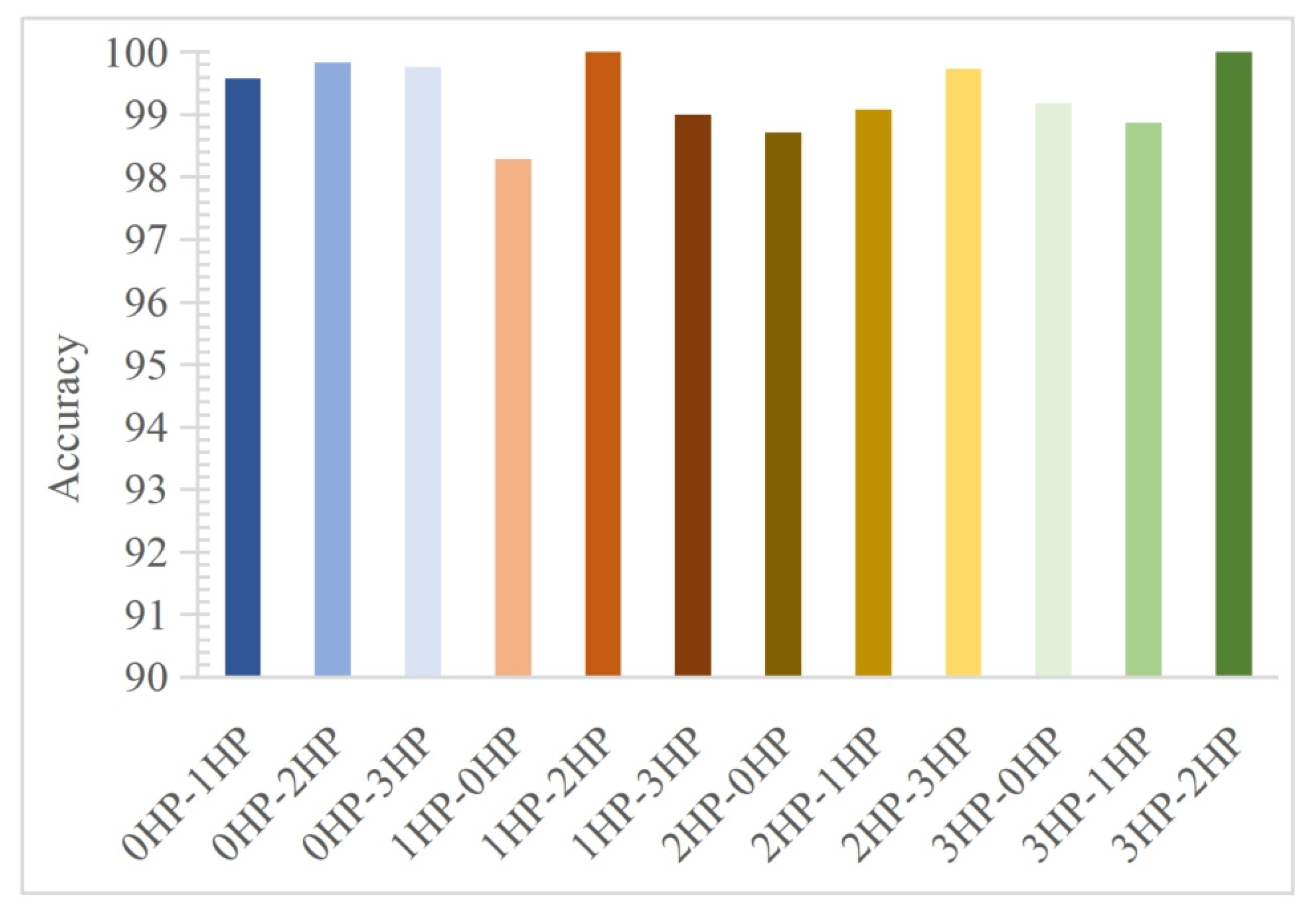
| 0HP-1HP | 32.74 | 34.61 | 98.84 | 99.58 |
| 0HP-2HP | 34.32 | 36.34 | 94.50 | 99.83 |
| 0HP-3HP | 36.61 | 40.09 | 99.06 | 99.77 |
| 1HP-0HP | 31.64 | 34.98 | 97.07 | 98.29 |
| 1HP-2HP | 34.50 | 37.63 | 99.30 | 100.00 |
| 1HP-3HP | 41.03 | 34.40 | 98.58 | 99.00 |
| 2HP-0HP | 33.72 | 37.64 | 96.33 | 98.71 |
| 2HP-1HP | 34.72 | 38.43 | 97.72 | 99.08 |
| 2HP-3HP | 35.63 | 35.09 | 99.59 | 99.74 |
| 3HP-0HP | 37.73 | 41.47 | 87.52 | 99.18 |
| 3HP-1HP | 39.51 | 37.67 | 98.38 | 98.87 |
| 3HP-2HP | 34.60 | 33.70 | 100.00 | 100.00 |
| mean | 35.56 | 36.84 | 97.24 | 99.34 |
| Source–Target Domain | MDE | RCMDE | RCMFDE | RCMVMFE | Frequency | MFF-IWBDA |
|---|---|---|---|---|---|---|
| 0HP-1HP | 86.92 | 99.21 | 92.30 | 99.66 | 66.03 | 99.58 |
| 0HP-2HP | 87.48 | 96.96 | 99.51 | 90.00 | 48.98 | 99.83 |
| 0HP-3HP | 76.70 | 96.12 | 79.31 | 79.82 | 80.47 | 99.77 |
| 1HP-0HP | 85.19 | 79.59 | 98.14 | 98.00 | 77.43 | 98.29 |
| 1HP-2HP | 94.42 | 99.71 | 99.90 | 99.50 | 88.29 | 100.00 |
| 1HP-3HP | 85.10 | 79.78 | 72.40 | 79.69 | 80.26 | 99.00 |
| 2HP-0HP | 87.96 | 97.60 | 82.72 | 78.89 | 58.81 | 98.71 |
| 2HP-1HP | 90.12 | 98.86 | 99.50 | 86.38 | 87.32 | 99.08 |
| 2HP-3HP | 89.06 | 93.64 | 99.57 | 98.92 | 85.83 | 99.74 |
| 3HP-0HP | 78.79 | 81.94 | 94.79 | 88.08 | 89.84 | 99.18 |
| 3HP-1HP | 80.82 | 79.29 | 79.61 | 88.52 | 76.36 | 98.87 |
| 3HP-2HP | 82.92 | 99.33 | 99.56 | 94.11 | 80.93 | 100.00 |
| mean | 85.46 | 91.84 | 91.44 | 90.13 | 76.71 | 99.34 |
| Source–Target Domain | RCMDE and RCMFDE | RCMDE, RCMFDE, and RCmvMFE | MDE, RCMDE, RCMFDE, and RCmvMFE | MFF-IWBDA |
|---|---|---|---|---|
| 0HP-1HP | 99.77 | 95.88 | 96.27 | 99.58 |
| 0HP-2HP | 91.47 | 82.08 | 82.21 | 99.83 |
| 0HP-3HP | 91.01 | 85.63 | 94.47 | 99.77 |
| 1HP-0HP | 99.49 | 98.72 | 98.33 | 98.29 |
| 1HP-2HP | 100.00 | 100.00 | 100.00 | 100.00 |
| 1HP-3HP | 82.62 | 79.16 | 79.19 | 99.00 |
| 2HP-0HP | 85.76 | 81.46 | 80.09 | 98.71 |
| 2HP-1HP | 99.46 | 99.44 | 99.24 | 99.08 |
| 2HP-3HP | 99.48 | 99.71 | 99.67 | 99.74 |
| 3HP-0HP | 99.20 | 95.17 | 94.41 | 99.18 |
| 3HP-1HP | 90.56 | 81.14 | 80.20 | 98.87 |
| 3HP-2HP | 99.62 | 99.76 | 99.96 | 100.00 |
| mean | 94.87 | 91.51 | 92.00 | 99.34 |
| Experiment | 0-1HP | 0-2HP | 0-3HP | 1-0HP | 1-2HP | 1-3HP | 2-0HP | 2-1HP | 2-3HP | 3-0HP | 3-1HP | 3-2HP |
|---|---|---|---|---|---|---|---|---|---|---|---|---|
| standard deviation (%) | 0.09 | 0.05 | 0.03 | 0.29 | 0 | 0.1 | 0.22 | 0.11 | 0.07 | 0.28 | 0.2 | 0 |
| Source–Target Domain | KMM | CORAL | GFK | MEDA | Easy-TL | Ea-CORAL | Ea-PCA | TCA | JDA | BDA | I-WBDA |
|---|---|---|---|---|---|---|---|---|---|---|---|
| 0HP-1HP | 20.00 | 27.82 | 86.04 | 90.89 | 85.11 | 85.92 | 84.97 | 82.48 | 93.61 | 98.84 | 99.58 |
| 0HP-2HP | 15.03 | 28.14 | 75.88 | 79.86 | 81.07 | 82.11 | 80.97 | 76.53 | 74.38 | 94.5 | 99.83 |
| 0HP-3HP | 20.00 | 62.89 | 76.4 | 80.34 | 78.51 | 76.41 | 79.18 | 69.46 | 86.51 | 99.06 | 99.77 |
| 1HP-0HP | 20.00 | 45.47 | 86.27 | 81.98 | 81.43 | 81.72 | 81.42 | 87.42 | 95.51 | 97.07 | 98.29 |
| 1HP-2HP | 19.90 | 30.51 | 94.43 | 91.72 | 89.5 | 90.14 | 89.01 | 91.01 | 99.5 | 99.3 | 100 |
| 1HP-3HP | 17.53 | 42.81 | 89.64 | 93.74 | 84.96 | 84.22 | 85.79 | 81.19 | 98.5 | 98.58 | 99 |
| 2HP-0HP | 11.90 | 53.09 | 79.13 | 77.63 | 81.94 | 82.13 | 81.91 | 80.41 | 71.28 | 96.33 | 98.71 |
| 2HP-1HP | 14.13 | 23.99 | 95.16 | 96.84 | 88.97 | 89.38 | 89.06 | 89.74 | 97.32 | 97.72 | 99.08 |
| 2HP-3HP | 20.00 | 48.98 | 89.6 | 97.66 | 92.69 | 92.7 | 92.49 | 78.78 | 89.41 | 99.59 | 99.74 |
| 3HP-0HP | 19.91 | 46.96 | 75.98 | 79.84 | 81.44 | 81.16 | 81.6 | 67.28 | 84.46 | 87.52 | 99.18 |
| 3HP-1HP | 12.19 | 35.72 | 74.54 | 90 | 85.02 | 87.68 | 85.08 | 76.67 | 97.79 | 98.38 | 98.87 |
| 3HP-2HP | 18.37 | 25.38 | 81.3 | 80.97 | 94.37 | 95.62 | 94.27 | 85.2 | 99.1 | 100 | 100 |
| mean | 17.41 | 39.31 | 83.7 | 86.79 | 85.42 | 85.77 | 85.48 | 80.51 | 90.61 | 97.24 | 99.34 |
| Literature | Year | Number of Working Conditions | Experiment | Accuracy (%) | Average Accuracy (%) | Number of Samples for Each Type of Fault |
|---|---|---|---|---|---|---|
| [29] | 2025 | 3 | 0-1 | 99.4 | 98.8 | 1000 |
| 0-2 | * 98.5 | |||||
| 0-3 | * 98.5 | |||||
| [45] | 2020 | 6 | 0-1,2 1-0,2 2-0,1 | 90.5 | 90.5 | 50 |
| [46] | 2025 | 12 | 0-1 | 97.82 | 93.89 | / |
| 0-2 | 91.72 | |||||
| 0-3 | 88.54 | |||||
| 1-0 | 99.25 | |||||
| 1-2 | 98.49 | |||||
| 1-3 | 91.06 | |||||
| 2-0 | 93.79 | |||||
| 2-1 | 93.77 | |||||
| 2-3 | 96.95 | |||||
| 3-0 | 83.82 | |||||
| 3-1 | 93.37 | |||||
| 3-2 | 98.14 | |||||
| [47] | 2025 | 6 | 1-2 | * 99.3 | 96.99 | 500 |
| 1-3 | * 97.5 | |||||
| 2-1 | * 94.1 | |||||
| 2-3 | * 98.8 | |||||
| 3-1 | * 94.4 | |||||
| 3-2 | * 97.9 | |||||
| [48] | 2017 | 6 | 1-2 | 99.4 | 95.9 | 685 |
| 1-3 | 93.4 | |||||
| 2-1 | 97.5 | |||||
| 2-3 | 97.2 | |||||
| 3-1 | 88.3 | |||||
| 3-2 | 99.9 | |||||
| The proposed method | / | 12 | 0-1 | 99.58 | 99.34 | 100 |
| 0-2 | 99.83 | |||||
| 0-3 | 99.77 | |||||
| 1-0 | 98.29 | |||||
| 1-2 | 100 | |||||
| 1-3 | 99 | |||||
| 2-0 | 98.71 | |||||
| 2-1 | 99.08 | |||||
| 2-3 | 99.74 | |||||
| 3-0 | 99.18 | |||||
| 3-1 | 98.87 | |||||
| 3-2 | 100 |
Disclaimer/Publisher’s Note: The statements, opinions and data contained in all publications are solely those of the individual author(s) and contributor(s) and not of MDPI and/or the editor(s). MDPI and/or the editor(s) disclaim responsibility for any injury to people or property resulting from any ideas, methods, instructions or products referred to in the content. |
© 2025 by the authors. Licensee MDPI, Basel, Switzerland. This article is an open access article distributed under the terms and conditions of the Creative Commons Attribution (CC BY) license (https://creativecommons.org/licenses/by/4.0/).
Share and Cite
Yang, J.; Bai, Y.; Xu, T.; Cheng, R.; Zhang, W.; Zhang, G. Complex Working Condition Bearing Fault Diagnosis Based on Multi-Feature Fusion and Improved Weighted Balance Distribution Adaptive Approach. Lubricants 2025, 13, 221. https://doi.org/10.3390/lubricants13050221
Yang J, Bai Y, Xu T, Cheng R, Zhang W, Zhang G. Complex Working Condition Bearing Fault Diagnosis Based on Multi-Feature Fusion and Improved Weighted Balance Distribution Adaptive Approach. Lubricants. 2025; 13(5):221. https://doi.org/10.3390/lubricants13050221
Chicago/Turabian StyleYang, Jing, Yanping Bai, Ting Xu, Rong Cheng, Wendong Zhang, and Guojun Zhang. 2025. "Complex Working Condition Bearing Fault Diagnosis Based on Multi-Feature Fusion and Improved Weighted Balance Distribution Adaptive Approach" Lubricants 13, no. 5: 221. https://doi.org/10.3390/lubricants13050221
APA StyleYang, J., Bai, Y., Xu, T., Cheng, R., Zhang, W., & Zhang, G. (2025). Complex Working Condition Bearing Fault Diagnosis Based on Multi-Feature Fusion and Improved Weighted Balance Distribution Adaptive Approach. Lubricants, 13(5), 221. https://doi.org/10.3390/lubricants13050221