1. Introduction
In recent years, the integration of machine learning (ML) into tribology has led to a paradigm shift in the understanding and optimization of friction, wear and lubrication phenomena [
1,
2,
3,
4]. A back-propagation neural network (BPNN) model has been developed to predict the wear performance of GCr15 steel. Validation experiments show that the average prediction error for the BPNN model is 10.64% [
5]. To improve the performance of tool wear detection, He et al. presented a novel semi-supervised method based on Long Short-Term Memory (LSTM) networks [
6]. Conventional methodologies depend on experimental reiterations or computationally intensive numerical simulations. They frequently encounter difficulties in achieving a balance between accuracy, efficiency and scalability in complex multi-parameter systems. Machine learning is a process that identifies nonlinear relationships and generalizes from limited data. These capabilities establish it as a transformative tool for predictive modeling in tribology. Recent advancements underscore the mounting influence of machine learning (ML) in the field of lubrication research. Physically informed neural networks (PINNs) have demonstrated their effectiveness in solving hydrodynamic and elastohydrodynamic lubrication (EHL) problems by incorporating physical laws into data-driven frameworks to ensure system robustness [
7,
8]. For example, Zhang et al. [
9] demonstrated that PINNs achieve less than 5% error in pressure distribution prediction for journal bearings, outperforming conventional finite element methods.
Supervised learning frameworks have been demonstrated to expedite the optimization of lubricant properties by leveraging structure-performance correlations. Examples of such methods include random forests and gradient-boosted trees [
10]. It is important to note that hybrid machine learning (ML) physics models are advancing dynamic lubrication analysis. For example, Wang et al. [
8] demonstrated that physics-informed neural networks (PINNs) enable the highly accurate prediction of elastohydrodynamic lubrication (EHL) film thickness under transient operating conditions. This approach overcomes the limitations of purely empirical models. The findings indicate a 22% decrease in computational time when compared to conventional finite element methods while maintaining over 95% accuracy in line contact scenarios.
In the field of biotribology, machine learning (ML) models have been employed to predict cartilage wear in artificial joints [
11] and to optimize synovial fluid substitutes [
12]. Bayesian optimization has emerged as a potent instrument for navigating high-dimensional parameter spaces in materials science. For instance, Snoek et al. [
13] demonstrated the efficacy of the method in the context of hyperparameter tuning for machine learning algorithms. In this scenario, surrogate models based on Gaussian processes were shown to reduce the computational cost by 50% in comparison with grid search methods.
Despite the success of machine learning (ML) in the field of synthetic lubricants and joint wear prediction, its application to aqueous bio-inspired lubricants remains limited due to their unique rheological complexity. While Bayesian optimization has been extensively used in chemical synthesis [
14], its potential in tuning neural networks for biotribological applications remains largely untapped. Hyperparameter sensitivity emerges as a significant obstacle in the field of tribological machine learning (ML) models in the context of non-Newtonian fluids. Existing machine learning (ML) models for lubrication often oversimplify the dynamic rheology of biofluids, thereby limiting their applicability to synthetic lubricants [
15].
In this work, we propose a Bayesian-optimized back-propagation (BP) neural network to predict the tribological performance of HA aqueous solutions in an inclined sliding contact under hydrodynamic lubrication conditions. The work presents the first implementation of Bayesian optimization in the context of automating hyperparameter tuning in biotribological lubrication modeling. This approach is shown to reduce training time compared to grid search methods. The model can predict the lubricating properties of HA under the condition of shear thinning behavior. A framework for rapid screening of HA formulations was validated. By integrating the fields of machine learning (ML) and biotribology, this study contributes to the advancement of data-driven lubricant design.
2. Experiment
2.1. Test Apparatus
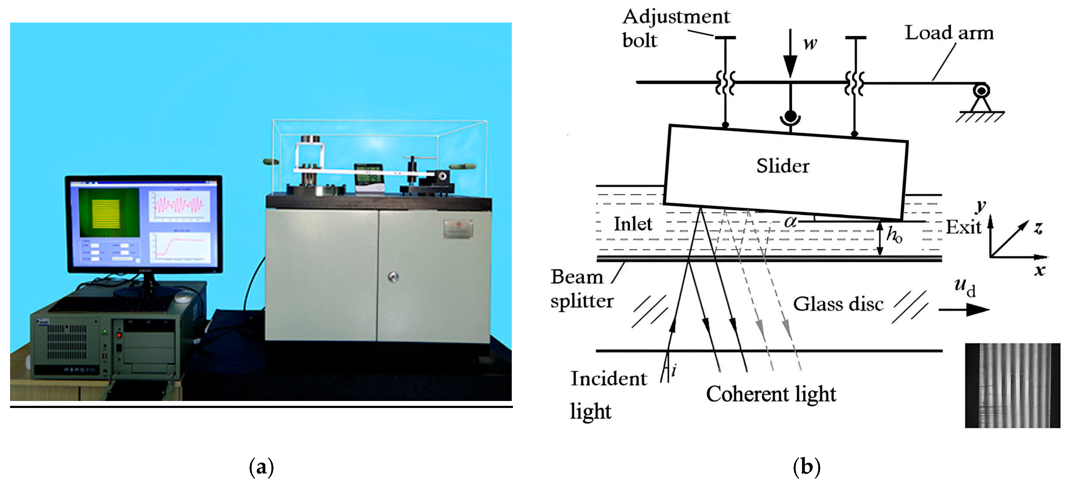
Figure 1a provides a photographic overview of the optical slider-bearing apparatus used in this study. In
Figure 1b, the schematic configuration of the experimental setup is presented along with the interference image obtained during the lubrication measurements. The lubrication interface consists of a stationary AISI 52100 steel slider and a rotating BK7 glass disc, with the latter exhibiting a surface roughness of
Ra = 4 nm. Interferometric measurements were conducted using a monochromatic light source (λ = 635 nm) [
16], projected perpendicular to the contact interface to generate multi-beam Fizeau interference patterns. To enable precise film thickness quantification, the glass disc surface was sequentially coated with a chromium (Cr) adhesion layer and a silicon dioxide (SiO
2) optical layer, forming an optimized beam-splitting interface [
17]. The steel slider surfaces were precision-polished to
Ra = 8 nm with λ/4 flatness tolerance. A controlled inclination angle (α) was achieved through an 8-bolt micro-adjustment mechanism integrated into the slider mounting assembly. The angular displacement was quantitatively determined from the number of interference fringes (
N) using the following relationship [
18]:
where
n is the refractive index of the lubricant, and
B is the breadth of the slider.
Under controlled operating conditions with the specified rotational speed ud and applied load w, the rotating glass disk generates a hydrodynamic lubrication regime between the contacting surfaces. The lubricating film is formed between the two surfaces. The glass disc rotates with a given speed ud and a load w, and a lubricating film is formed between the two surfaces because of the hydrodynamic effect. In the test, the film thickness is represented by the minimum film thickness h0 at the exit.
Load-carrying capacity is a crucial parameter in the study of hydrodynamic lubrication theory. Typically, the relationship between dimensionless load and convergence ratio is used to characterize the lubrication performance of the slider bearings. This current test apparatus can be used to obtain the load-carrying capacity of the lubricant film [
19].
According to the classical lubrication theory [
20], the dimensionless load is described by the following equation:
where
w the load per unit length (N/m),
h0 is the outlet oil thickness (m),
η denotes the dynamic viscosity of the lubricant (Pa s),
ud is the sliding speed (m/s) and
B refers to the slider width (m). A capacity of 6
W is commonly used to characterize the load-carrying capacity of sliding bearings [
20].
2.2. Lubricant Samples and Test Conditions
The experimental conditions are designed to satisfy hydrodynamic lubrication criteria while remaining within the operational limits of the test apparatus. Considering the design constraints of the experimental apparatus, a slider was used in the experiment. The working surface of the steel slider was polished to a high-precision finish, with a breadth of 4 mm in the sliding direction and a length of 10 mm. The sliding occurs along the width of the slider. In the experimental setup, sodium hyaluronate and deionized water were utilized as lubricants. The sodium hyaluronate used in the experiment was pharmaceutical-grade. The molecular weight of sodium hyaluronate ranges from approximately 0.8 to 2.0 million Daltons, and two different solutions with varying viscosities were prepared by adjusting the ratios of sodium hyaluronate to deionized water. The dynamic viscosity of the solutions was measured using a rotational rheometer with controlled shear rates at 25 °C. The speed and load ranges were selected to ensure the formation of a stable oil film during the experimental process. The test conditions applied, along with the lubricant properties, are detailed in
Table 1.
2.3. Preparation of the Dataset
In the context of hydrodynamic lubrication, the thickness of the lubricant film depends on several factors, including the load, the speed, the slider inclination and the lubricant viscosity. The test conditions used in the measurements are described in
Table 1. A total of 128 film thickness measurements were obtained under a range of test conditions. Subsequently, the dimensionless load-carrying capacity was determined. The establishment of a sample dataset was subsequently initiated.
In the context of the fundamental BP network, the data were segmented into two distinct sets: a training dataset, constituting 80% of the total data, and a test dataset, comprising the remaining 20%. In the Bayesian-optimized BP network, an additional validation dataset (20%) was extracted from the original training data, resulting in a final partition ratio of 0.6:0.2:0.2 (train/validation/test). This procedure facilitated the training and evaluation of the effectiveness of the neural network model.
3. BP Neural Network and Optimization
3.1. BP Neural Network
A BP neural network is a multi-layer feed-forward network that employs the back-propagation learning algorithm to adjust the connection weights of its neurons. The algorithm employs the error back-propagation method, whereby the network follows a gradient descent learning rule. This process of continuous adjustment of weights and thresholds, facilitated by back-propagation, is instrumental in minimizing the sum of squared errors across the network [
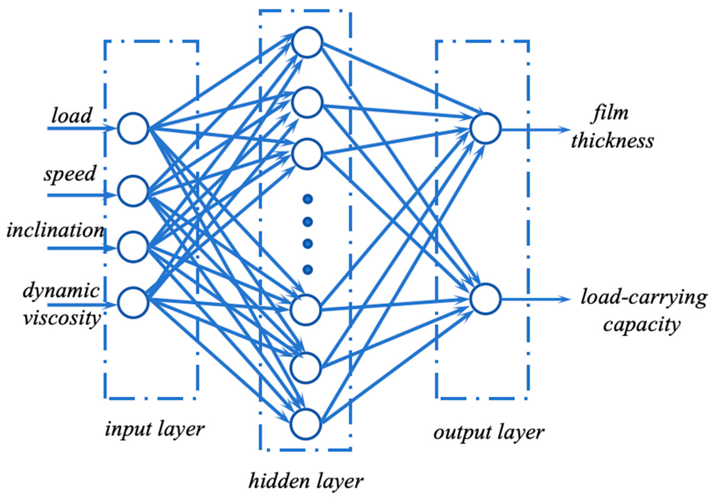
21]. The topology of a BP neural network model consists of an input layer, one or more hidden layers and an output layer. The presence of hidden layers contributes to the capacity of the network for strong nonlinear mapping. Preliminary theoretical studies have demonstrated the potential of a three-layer BP neural network to approximate any nonlinear continuous function with a high degree of accuracy [
22]. This renders BP neural networks particularly well-suited for addressing problems with complex internal mechanisms [
23]. The network under consideration in this paper features a hidden layer network structure with four inputs and two outputs. The network model’s structure is illustrated in
Figure 2.
The hidden layer utilizes a sigmoid activation function, whereas the output layer employs a linear activation function. The optimal number of hidden layer nodes must be determined with care. Insufficient hidden nodes can hinder the network’s capacity to effectively capture intricate relationships, whereas an excess of hidden nodes can result in overfitting. Currently, there is no definitive method for determining the ideal number of hidden layer nodes. The design of hidden layer architecture requires careful consideration of the problem’s inherent complexity, including the nonlinearity of input–output relationships and dataset characteristics. Since the input/output dimension is a preliminary reference for regression tasks, we referred to empirical formulas to preliminarily set the number of neurons [
24]. Finally, the number of hidden layer nodes was set to ten. Following this initial determination, a trial-and-error approach was employed, whereby parameters were manually adjusted to gradually increase the number of nodes. This iterative process was repeated until the configuration that yielded the optimal fitting performance was identified. Once the optimal number of hidden layer nodes was established, the learning rate was adjusted to control the model’s convergence speed and stability. It is important to note that an overly large learning rate may result in oscillation and divergence, whereas an excessively small learning rate may lead to slow convergence. It is therefore crucial to select an appropriate learning rate in order to achieve effective model training. The initial learning rate was set to 0.01. Later, it was manually adjusted based on the performance indicators of the network.
3.2. Implementing the BP Neural Network Model
Python 3.6 is the development language of the network model. PyCharm 2023.3.5 is the integrated development platform. The parameters of the network model were initially set, and the training samples were fed into the system. The gradient descent algorithm was used to train the network. As the input parameters—load, inclination, viscosity and speed—have different dimensions and significant differences in order of magnitude, it is necessary to pre-process the original data to mitigate the effects of these discrepancies and increase the training speed of the network. This is achieved by data normalization. Max-min normalization is used for data pre-processing to map data with different dimensions and units to a unified scale [
25]. This method preserves the relationships within the original data and is the simplest approach to eliminating the effects of different dimensions and value ranges. The formula is defined by Equation (3):
where
Xin is the original data point,
Xmin is the minimum,
Xmax is the maximum and
X* is the normalized data point. In the study, the whole sample set was normalized.
The MSE was chosen as the training objective. The MSE is an indicator used to measure the predictive power of a model. It is calculated as follows:
where
j is the number of samples in the dataset,
yi is the true value of the
ith sample and
i is the predicted value of the
ith sample. The mean square error is calculated by first squaring the difference between the predicted value and the true value for each sample then adding the square variances for all samples and dividing by the number of samples
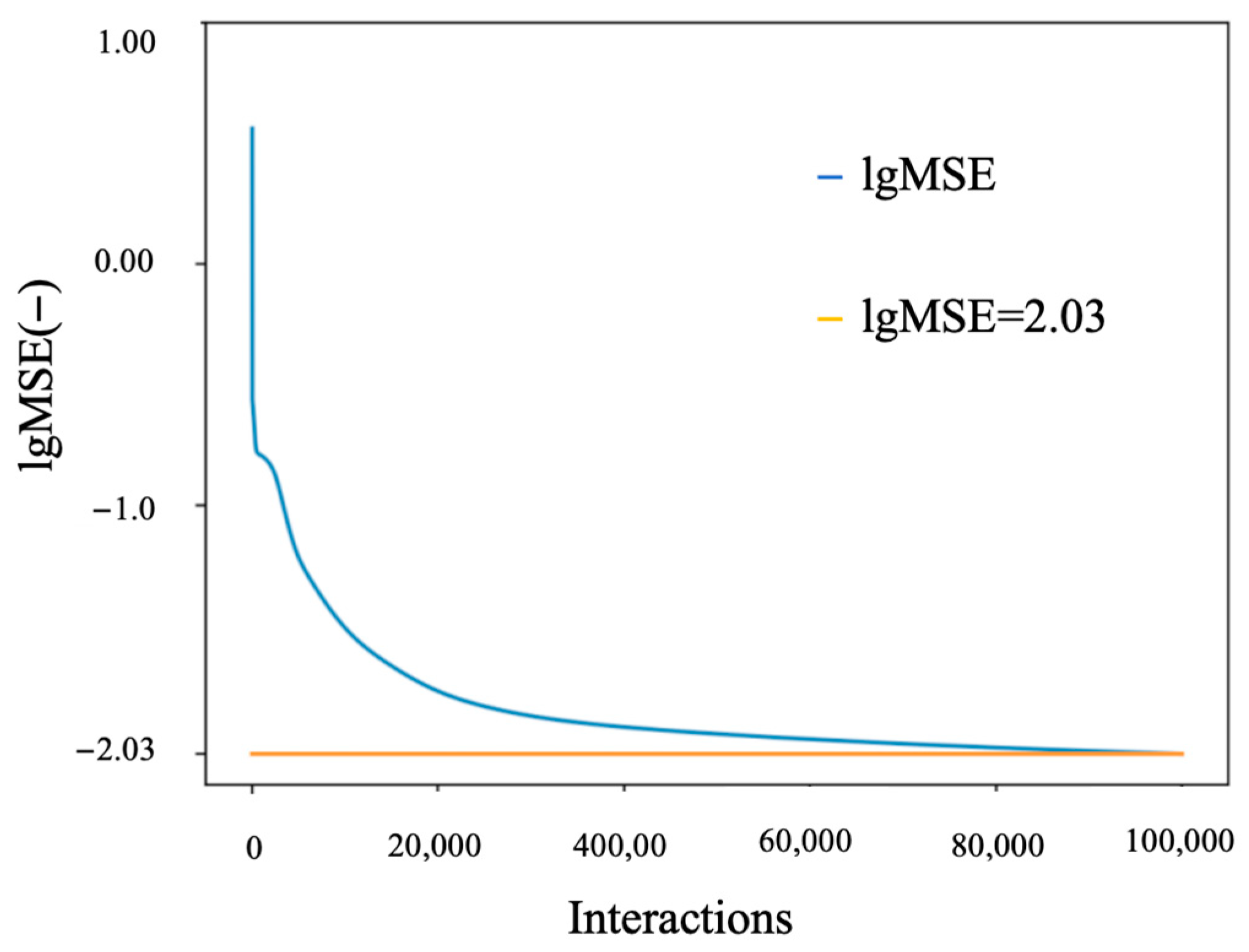
j. In machine learning and deep learning, MSE is often used as an evaluation metric for regression models. A minimum MSE threshold of 0.001 was set to ensure convergence and stability in training. Subsequent to the conclusion of the training process, the network output results were reverse-normalized in order to obtain the actual output values. The error change curve during the network training process is presented in
Figure 3. As illustrated in
Figure 3, the MSE decreases rapidly during the initial training stage and then tapers off more slowly with an increase in training iterations. After nearly 10
5 training cycles, the MSE of the model stabilizes at around 0.01.
3.3. Bayesian Optimization
The prediction capability of the BP neural network model is contingent upon the configuration of its hyperparameters, which in turn determines the model’s accuracy and efficiency. During the training process of the BP network model, manual adjustment of parameters is necessary to identify the optimal configuration. Such parameters include the number of neurons, the number of iterations and the learning rate. However, this method is susceptible to converging on a local minimum rather than achieving a global optimum. Furthermore, studies have shown that excessive training iterations may reduce learning efficiency and lead to slower convergence. To address these challenges and enhance the efficiency of the training process, a Bayesian optimization algorithm was employed to optimize the network model. Bayesian optimization is a global optimization algorithm that serves as an effective method for hyperparameter tuning. The fundamental principle of Bayesian optimization is predicated on the utilization of conditional probability in order to transform the prior probability model into a posterior probability distribution [
26], thus enabling the active selection of the subsequent local point. The theoretical underpinnings of Bayesian optimization are rooted in Bayes’ theorem, which employs Bayes’ public formula to establish the probability distribution of the optimization process [
27].
In Equation (5),
f denotes the unknown objective function to be optimized;
D = {(
x1,
y1), (
x2,
y2), …, (
xn,
yn)} represents the observed dataset, where
xi is the decision vector,
yi =
f (
xi) +
εi is the observed value and
εi is the observation error typically assumed to follow a Gaussian distribution; and the likelihood
p(
D|
f) models the probability of observing
y given
f, while
p(
f) represents the prior distribution encoding assumptions about
f. The marginal likelihood
p(
D), defined as the integral of the product of likelihood and prior over all possible
f, is critical for hyperparameter optimization but computationally intractable for complex models. Modern Bayesian optimization frameworks such as scikit-optimize [
28] and GPyOpt [
29] address this challenge through computational strategies. For Gaussian process surrogates, hyperparameters are optimized by maximizing the marginal likelihood via gradient-based methods [
13]. To enhance scalability, these frameworks implement sparse approximations and stochastic variational inference [
30], reducing computational complexity.
The Bayesian optimization framework uses a probabilistic surrogate model and an acquisition function to efficiently explore the parameter space. By iteratively constructing a Gaussian process (GP) model of the objective function and using the Expected Improvement (EI) acquisition strategy, this method balances exploration and exploitation, enabling rapid convergence to the optimal hyperparameter [
31].
In the present study, the Bayesian Optimization Library was used, with convergence requiring a normalized validation MSE below 0.001 or a maximum of 300 epochs. Bayesian optimization selected the number of hidden neurons (10~120), while training was terminated by stopping early if the validation loss failed to improve for 20 epochs, with a safety cap of 300 epochs. The initial learning rate was selected by Bayesian optimization from a range (10
−5~10
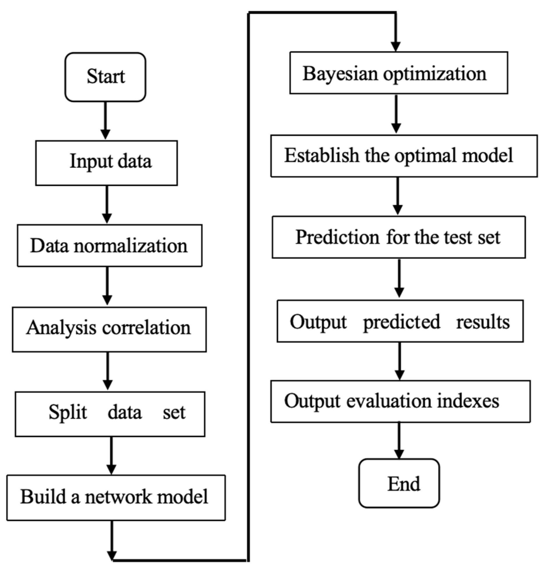
−2), while the Adam optimizer adjusted it dynamically during training based on gradient moments. As demonstrated in
Figure 4, the Bayesian-optimized BP neural network was then used to predict HA lubrication characteristics. This approach resulted in a significant reduction in manual hyperparameter tuning effort while improving model accuracy and generalizability.
4. Results and Discussion
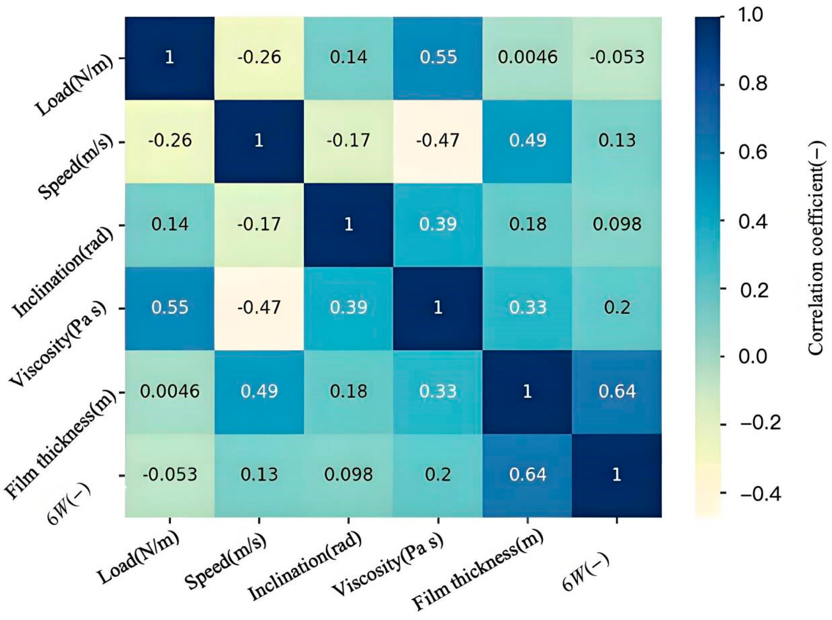
Figure 5 presents the heatmap illustrating the correlation of experimental data. Here, we only focus on the correlation between input and output. The heatmap provides a visual representation of the strength of the correlation between the input and output variables. It is evident that the thermal map reflects the potential correlation law in the dataset. As shown in
Figure 5, within the parameter range we studied, the heatmap reveals significant positive correlations between sliding velocity and lubricant viscosity with both film thickness and bearing capacity. This lays the foundation for enhancing lubrication characteristics.
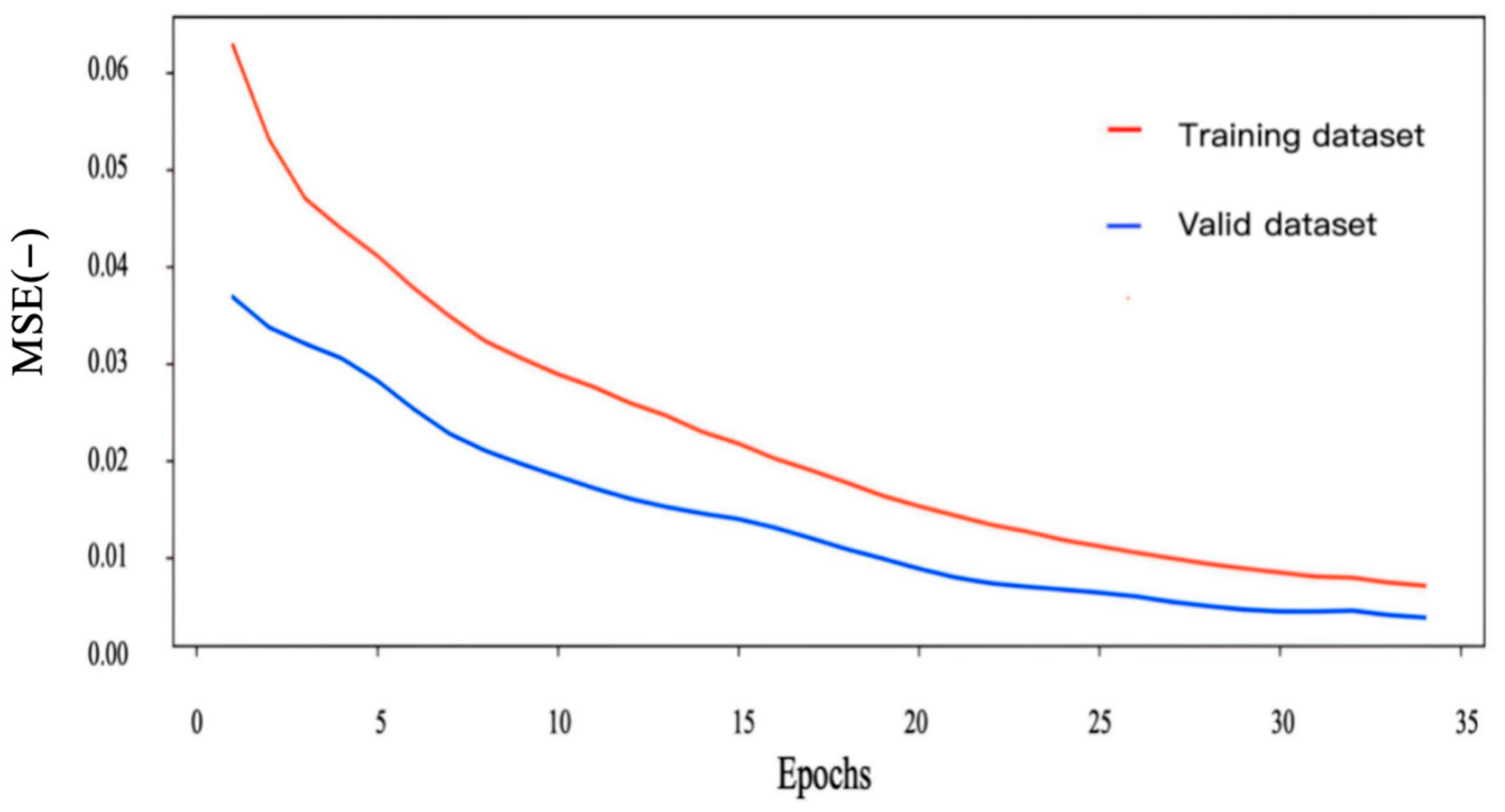
As illustrated in
Figure 6, the MSE curves of the Bayesian-optimized BP neural network demonstrate consistent convergence. The training MSE demonstrates a downward trend, decreasing monotonically with increasing epochs. After 30 training cycles, the MSE stabilizes below 0.01. It is noteworthy that the validation MSE (red line) remains below the training MSE throughout the process, indicating that there is no occurrence of overfitting and that generalization is robust. This behavior is consistent with the early stopping criterion, which was implemented to prevent the unnecessary continuation of training beyond the convergence point.
The precipitous decline in MSE within the initial 10 epochs (from 0.1 to 0.03) substantiates the efficacy of Bayesian optimization in directing hyperparameter selection. In comparison with the conventional grid search, the proposed method demonstrated equivalent accuracy after 30 epochs. These results validate the model’s readiness for predictive applications in HA lubrication analysis.
In order to validate the model, the film thickness and load-carrying capacity (6
W) of the test dataset were predicted. In this study, 20% of the data were allocated for the test dataset. As illustrated in
Figure 7, there is a clear demonstration of the relationship between true values and predicted values. As demonstrated in
Figure 7a, the
x-axis is indicative of the true value of film thickness, while the
y-axis is indicative of the predicted value of film thickness. As demonstrated in
Figure 7b, the
x-axis signifies the true load-bearing capacity (6
W), while the
y-axis indicates the predicted value of the load-bearing capacity (6
W). It is evident that the predicted value exhibits a close alignment with x = y.
The quantitative performance of this model is evidenced by its coefficient of determination (R2), which achieves a value of 0.938 on the test dataset. The result is consistent with the performance of PINNs in synthetic lubricant studies. Concurrently, the MSE is recorded at 0.0025, indicative of the precision and accuracy of this model. These metrics serve to substantiate the capacity of this model to accurately replicate hydrodynamic lubrication behavior. The results demonstrate comparable accuracy for HA aqueous solutions.
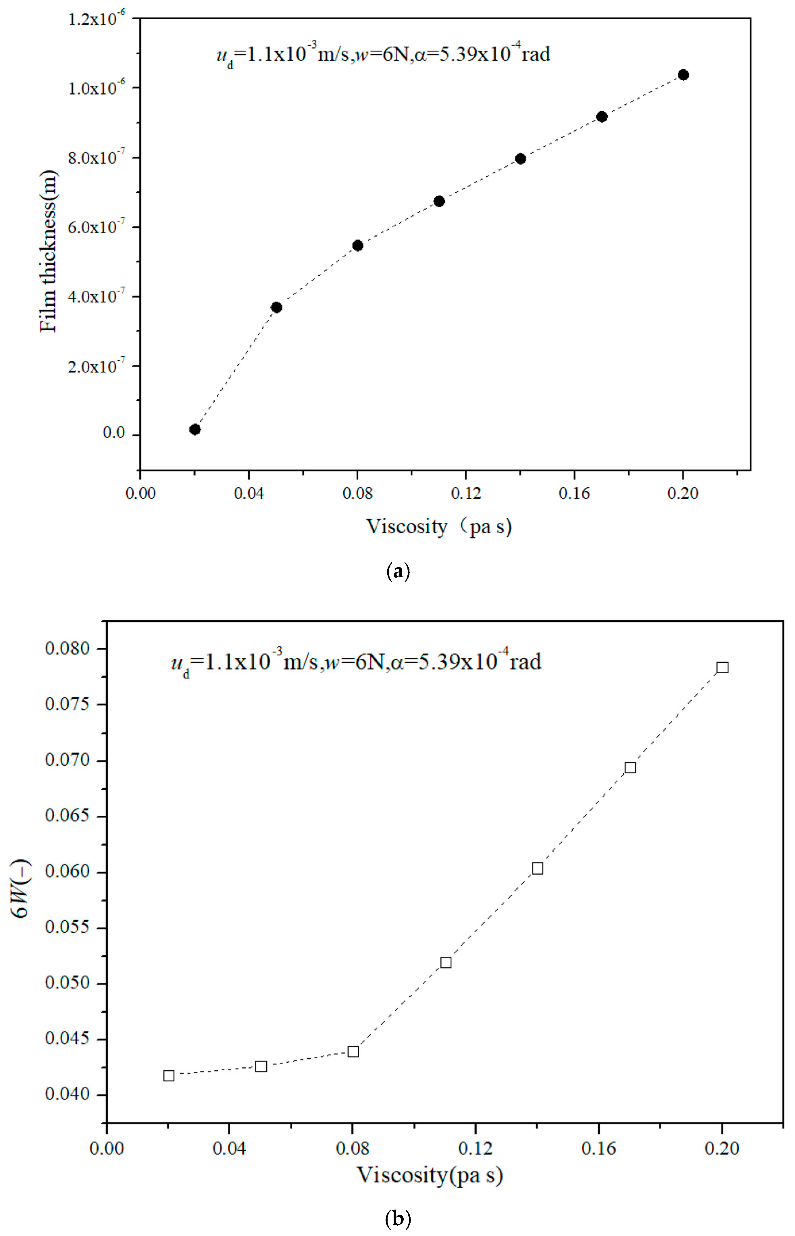
The model has been demonstrated to predict film thickness and load-carrying capacity within the constrained range of input parameters for training samples. As illustrated in
Figure 5, the correlation coefficient between viscosity, film thickness and load-bearing capacity is relatively high. Viscosity alterations have been shown to have a substantial impact on the thickness and load-carrying capacity of the film. Consequently, within the viscosity range delineated by the model training samples, the model was employed to predict the lubrication characteristics of HA aqueous solutions with varying viscosities. The value of viscosity is between 0.02 and 0.9. The relationship between the curve of the film thickness and the load-carrying capacity of HA aqueous solution as a function of viscosity is illustrated in
Figure 8. As demonstrated in
Figure 8, it is evident that the film thickness and dimensionless load-carrying capacity of the HA aqueous solution exhibit a proportional relationship with the increase in viscosity. The result contributes to the enhancement of the credibility of the proposed model.
5. Conclusions
This study proposes a Bayesian-optimized BP neural network framework for predicting the tribological performance of HA aqueous solutions under hydrodynamic lubrication conditions. The integration of Bayesian optimization with a BP neural network can address challenges in hyperparameter tuning and dynamic rheological modeling. This integration provides an efficient solution for biotribological applications.
The Bayesian-optimized BP neural network demonstrated a high degree of prediction accuracy, as evidenced by a coefficient of determination (R2) of 0.938 and a MSE of 0.0025 on the test dataset. This performance underscores the framework’s ability to capture the nonlinear relationships between HA aqueous solution characteristics and tribological outcomes. The model can be used for the prediction of the lubricant properties of HA aqueous solution without the need for experimentation and computation.
Bayesian optimization was shown to significantly reduce the need for manual tuning efforts by automating the selection of critical hyperparameters. The convergence of the MSE to less than 0.01 within 30 training iterations. It illustrates the effectiveness of this approach compared to conventional grid search methods. Bayesian optimization can be used in the predicted model of biotribological lubrication.
The model demonstrated a robust positive correlation between viscosity and lubrication performance, thereby validating the hypothesis derived from hydrodynamic theory and demonstrating the applicability of the model to non-Newtonian biofluids.
Author Contributions
Conceptualization, X.L.; methodology, X.L. and F.G.; software, X.L.; validation, X.L. and F.G.; formal analysis, X.L. and F.G.; investigation, X.L.; data curation, X.L.; writing—original draft preparation, X.L.; writing—review and editing, X.L. and F.G.; supervision, X.L. and F.G.; funding acquisition, F.G. All authors have read and agreed to the published version of the manuscript.
Funding
This research was funded by the Natural Science Foundation of China, grant number 52275196.
Data Availability Statement
The data used to support the findings of this study are included in the manuscript.
Conflicts of Interest
The authors declare no conflicts of interest.
Abbreviations
The following abbreviations are used in this manuscript:
| BP | back-propagation |
| HA | hyaluronic acid |
| ML | machine learning |
| PINNs | physics-informed neural networks |
| EHL | elastohydrodynamic lubrication |
| MSE | mean square error |
References
- Xia, Y.Q.; Wang, C.L.; Feng, X. Prediction of friction and wear performance of lubricating oil based on GRNN optimized by GWO. Tribology 2022, 43, 947–955. [Google Scholar]
- Zhao, Y.C.; Hao, G.J. Friction and wear properties analysis of plasma spraying coating based on the BP neural network. Lubr. Eng. 2013, 38, 10–13. [Google Scholar]
- Ma, M.M.; Fu, Y.W. Prediction model for sliding friction properties of friction materials based on BP neural network. Lubr. Eng. 2019, 44, 58–62. [Google Scholar]
- Sieberg, P.M.; Kurtulan, D.; Hanke, S. Wear Mechanism Classification Using Artificial Intelligence. Materials 2022, 15, 2358. [Google Scholar] [CrossRef] [PubMed]
- He, T.; Chen, W.; Liu, Z.; Gong, Z.; Du, S.; Zhang, Y. The Impact of Surface Roughness on the Friction and Wear Performance of GCr15 Bearing Steel. Lubricants 2025, 13, 187. [Google Scholar] [CrossRef]
- He, X.; Zhong, M.; He, C.; Wu, J.; Yang, H.; Zhao, Z.; Yang, W.; Jing, C.; Li, Y.; Gao, C. A Novel Tool Wear Identification Method Based on a Semi-Supervised LSTM. Lubricants 2025, 13, 72. [Google Scholar] [CrossRef]
- Raissi, M.; Perdikaris, P.; Karniadakis, G.E. Physics-informed neural networks: A deep learning framework for solving forward and inverse problems involving nonlinear partial differential equations. J. Comput. Phys. 2019, 378, 686–707. [Google Scholar] [CrossRef]
- Wang, Y.; Zhang, L.; Liu, G. Physics-informed neural networks for elastohydrodynamic lubrication analysis of line contacts. Tribol. Int. 2022, 175, 107823. [Google Scholar]
- Zhang, H.; Li, Q.; Wang, J. Machine learning-based pressure prediction in hydrodynamic journal bearings: A comparative study of PINNs and FEM. Wear 2023, 522–523, 204930. [Google Scholar]
- Smith, R.J.; Lee, S.H. Data-driven optimization of synthetic lubricants using gradient-boosted regression trees. J. Tribol. 2021, 143, 051801. [Google Scholar]
- Chen, X.; Liu, Y.; Gupta, S. Predicting cartilage wear in artificial joints via convolutional neural networks: A biotribological perspective. Biotribology 2023, 33, 100215. [Google Scholar]
- Kumar, A.; Patel, V.; Williams, R.L. Machine learning-guided design of synovial fluid substitutes with tunable rheological properties. ACS Appl. Mater. Interfaces 2022, 14, 50812–50825. [Google Scholar]
- Snoek, J.; Larochelle, H.; Adams, R.P. Practical Bayesian Optimization of Machine Learning Algorithms. Adv. Neural Inf. Process. Syst. 2012, 25, 2951–2959. [Google Scholar]
- Shields, B.J.; Stevens, J.; Li, J.; Parasram, M.; Damani, F.; Alvarado, J.I.M.; Janey, J.M.; Adams, R.P.; Doyle, A.G. Bayesian reaction optimization as a tool for chemical synthesis. Nature 2021, 590, 89–96. [Google Scholar] [CrossRef] [PubMed]
- Balazs, E.A.; Denlinger, J.L. Viscosity augmentation in hyaluronic acid solutions: Implications for synovial fluid function. J. Rheumatol. 1993, 20, 3–9. [Google Scholar]
- Guo, F.; Wong, P.L. A multi-beam intensity-based approach for lubricant film measurements in non-conformal contacts. Part J J. Eng. Tribol. 2002, 216, 281–291. [Google Scholar] [CrossRef]
- Ma, C.; Guo, F.; Fu, Z.X.; Yang, S.Y. Measurement of lubricating oil film thickness in conformal Contacts. Tribology 2010, 30, 419–424. [Google Scholar]
- Spikes, H.A.; Guangteng, G. An experimental study of film thickness in the mixed lubrication regime. Tribol. Trans. 1993, 36, 689–699. [Google Scholar]
- Li, X.; Guo, F.; Yang, S.Y. Measurement of load-carrying capacity of thin lubricating films. Tribology 2012, 32, 139–143. [Google Scholar] [CrossRef]
- Hamrock, B.J.; Schmid, S.R.; Jacobson, B.O. Fundamentals of Fluid Film Lubrication, 2nd ed.; CRC Press: Boca Raton, FL, USA, 2004; pp. 170–175. [Google Scholar]
- Liu, Z.Y.; He, T.T.; Gong, Z.P.; Li, J.F. Prediction of surface wear trend of GCr15 bearing steel based on BP neural network. Trans. Mater. Heat Treat. 2023, 44, 174–183. [Google Scholar]
- Cybenko, G. Approximation by superpositions of a sigmoidal function. Math. Control Signals Syst. 1989, 2, 303–314. [Google Scholar] [CrossRef]
- Pang, W.C.; Liu, S.D. Optimization research and application of BP neural network. Comput. Technol. Dev. 2019, 29, 74–76+101. [Google Scholar]
- Wang, R.B.; Xu, H.Y.; Li, B.; Feng, Y. Research on method of determining hidden layer nodes in BP neural network. Comput. Technol. Dev. 2018, 28, 31–35. [Google Scholar]
- Shaik, N.; Benjapolakul, W.; Pedapati, S.; Bingi, K.; Le, N.; Asdornwised, W.; Chaitusaney, S. Recurrent neural network-based model for estimating the life condition of a dry gas pipeline. Process Saf. Environ. Prot. 2022, 164, 639–650. [Google Scholar] [CrossRef]
- Sun, B.; Chu, F.F.; Chen, X.H. Non-invasive blood pressure detection method based on Bayesian optimization on XGBoost. Electron. Meas. Technol. 2022, 45, 68–74. [Google Scholar]
- Wu, J.; Chen, X.Y.; Zhang, H.; Xiong, L.D.; Lei, H.; Deng, S.H. Hyperparameter Optimization for Machine Learning Models Based on Bayesian Optimization. J. Electron. Sci. Technol. 2019, 17, 26–40. [Google Scholar]
- Head, T.; Kumar, M.; Louppe, G. scikit-optimize: Sequential model-based optimization in Python. J. Open Source Softw. 2020, 5, 2461. [Google Scholar]
- González, J.; Dai, Z.; Hennig, P.; Lawrence, N. GPyOpt: A Bayesian optimization framework in Python. J. Mach. Learn. Res. 2016, 7, 1–5. [Google Scholar]
- Cui, J.X.; Yang, B. A review of Bayesian optimization methods and applications. J. Softw. 2018, 29, 3068–3090. [Google Scholar]
- Vargas-Hernandez, R.A. Bayesian Optimization for Calibrating and Selecting Hybrid-Density Functional Models. J. Phys. Chem. A 2020, 124, 4053–4061. [Google Scholar] [CrossRef]
| Disclaimer/Publisher’s Note: The statements, opinions and data contained in all publications are solely those of the individual author(s) and contributor(s) and not of MDPI and/or the editor(s). MDPI and/or the editor(s) disclaim responsibility for any injury to people or property resulting from any ideas, methods, instructions or products referred to in the content. |
© 2025 by the authors. Licensee MDPI, Basel, Switzerland. This article is an open access article distributed under the terms and conditions of the Creative Commons Attribution (CC BY) license (https://creativecommons.org/licenses/by/4.0/).


