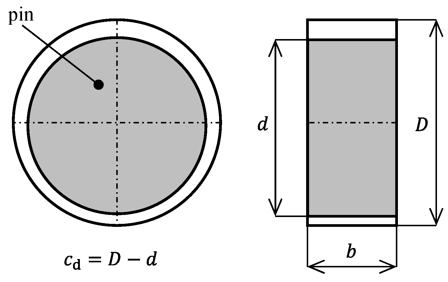
Figure 1.
Definition of the dimensions of a HD journal bearing, where is the journal diameter, is the shell diameter, is the journal width and is the bearing clearance.
Figure 1.
Definition of the dimensions of a HD journal bearing, where is the journal diameter, is the shell diameter, is the journal width and is the bearing clearance.
Figure 2.
Definition of the dimensions of the working surface of one thrust bearing segment. The symbol represents the number of segments, is the inner radius of the working surface, is the outer radius of the working surface, is the inner radius of the tapered part, is the outer radius of the tapered part, is the taper wedge angle, is the limit wedge angle of the tapered part, is the groove height, is the taper part angle, and is the angle of the lubricating groove.
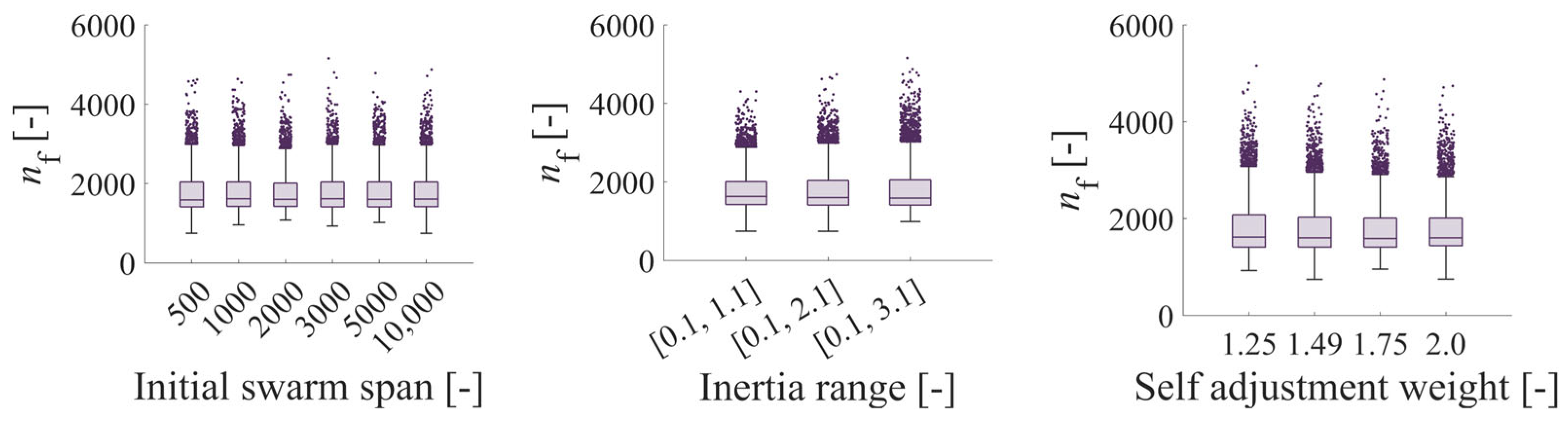
Figure 3.
Effect of Initial swarm span, minimum neighbours fraction and Inertia range on the number of expressions of the objective function in the case of PSWM using the analytical solution of the journal bearing.
Figure 3.
Effect of Initial swarm span, minimum neighbours fraction and Inertia range on the number of expressions of the objective function in the case of PSWM using the analytical solution of the journal bearing.
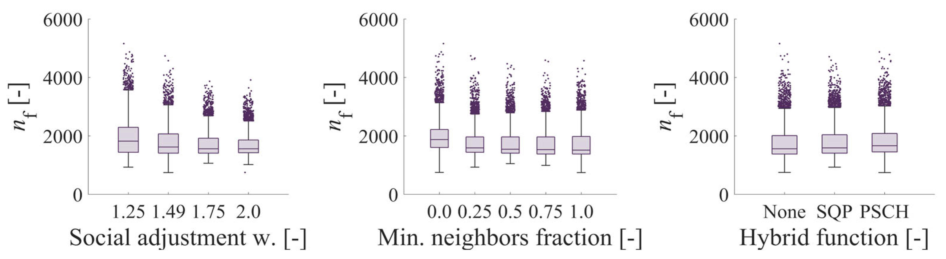
Figure 4.
Effect of Self adjustment weight, Social adjustment weight and Hybrid function on the number of expressions of the objective function in the case of PSWM using the analytical solution of the journal bearing.
Figure 4.
Effect of Self adjustment weight, Social adjustment weight and Hybrid function on the number of expressions of the objective function in the case of PSWM using the analytical solution of the journal bearing.
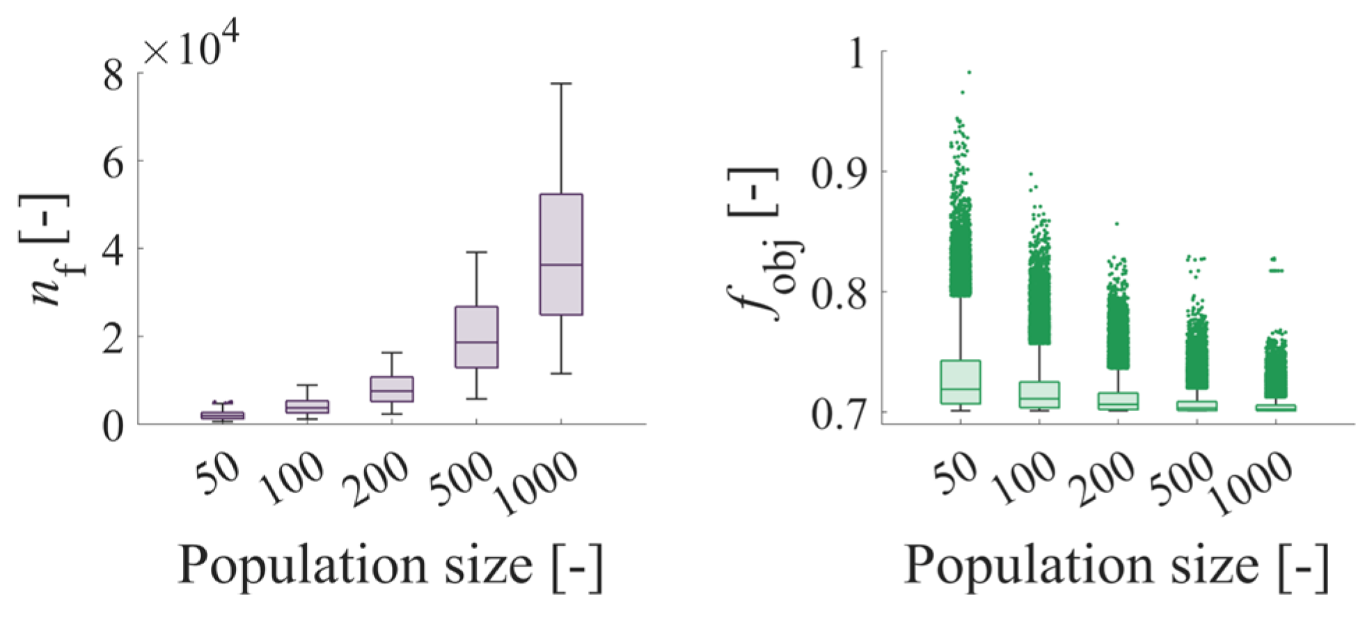
Figure 5.
Effect of population size on the number of objective function expressions and its value in the GA case using the analytical solution of the journal bearing.
Figure 5.
Effect of population size on the number of objective function expressions and its value in the GA case using the analytical solution of the journal bearing.
Figure 6.
Effect of the type of crossover function on the number of objective function expressions and its value in the case of GA using the analytical solution of the journal bearing.
Figure 6.
Effect of the type of crossover function on the number of objective function expressions and its value in the case of GA using the analytical solution of the journal bearing.
Figure 7.
Effect of Mutation function type on the number of expressions of the objective function and its value in the case of GA using the analytical solution of journal bearing.
Figure 7.
Effect of Mutation function type on the number of expressions of the objective function and its value in the case of GA using the analytical solution of journal bearing.
Figure 8.
Effect of the selection function on the number of expressions of the objective function and its value in the case of GA using the analytical solution of the journal bearing.
Figure 8.
Effect of the selection function on the number of expressions of the objective function and its value in the case of GA using the analytical solution of the journal bearing.
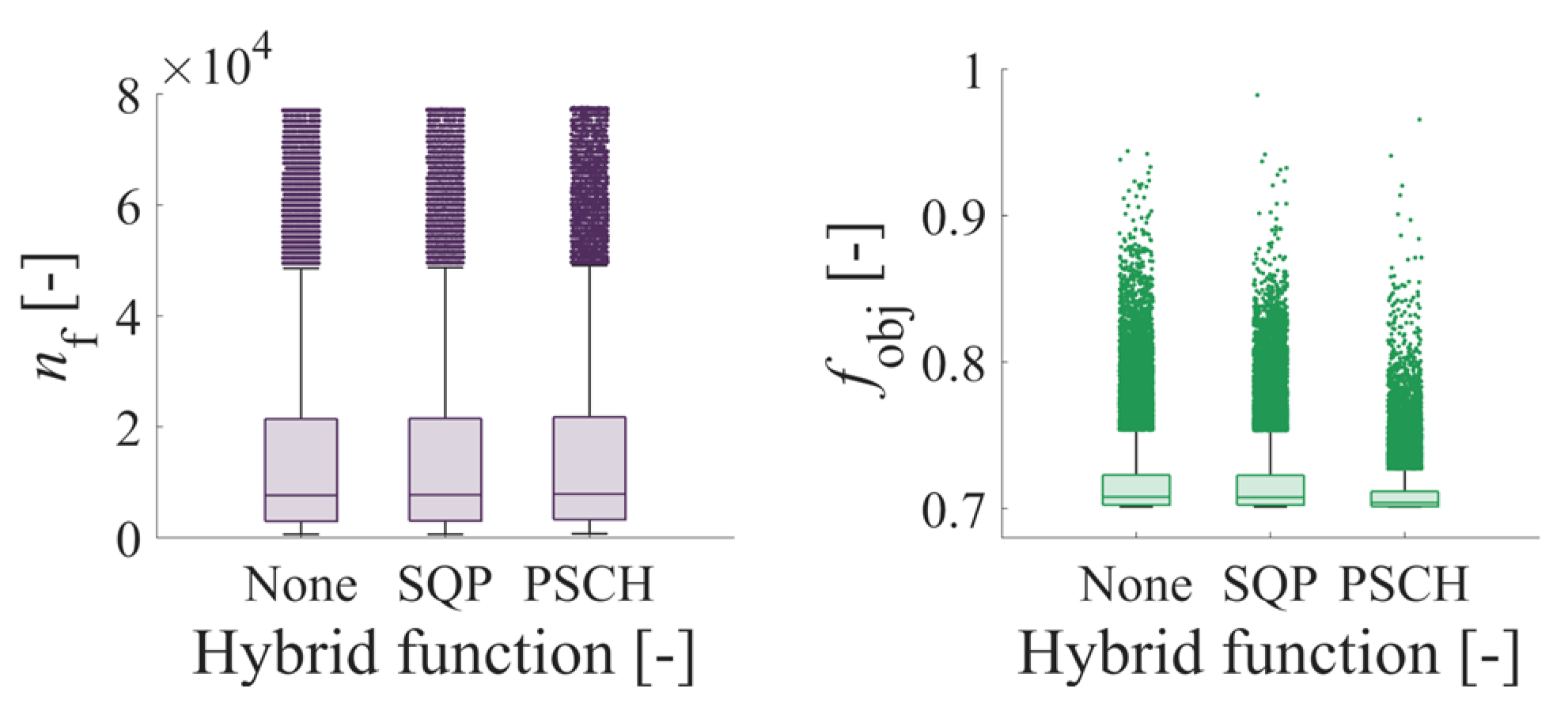
Figure 9.
Effect of Hybrid function type on the number of expressions of the objective function and its value in the GA case using the analytical solution of journal bearing.
Figure 9.
Effect of Hybrid function type on the number of expressions of the objective function and its value in the GA case using the analytical solution of journal bearing.
Figure 10.
Effect of algorithm type on the number of expressions of the objective function and its value in the case of PSCH using the analytical solution of journal bearing.
Figure 10.
Effect of algorithm type on the number of expressions of the objective function and its value in the case of PSCH using the analytical solution of journal bearing.
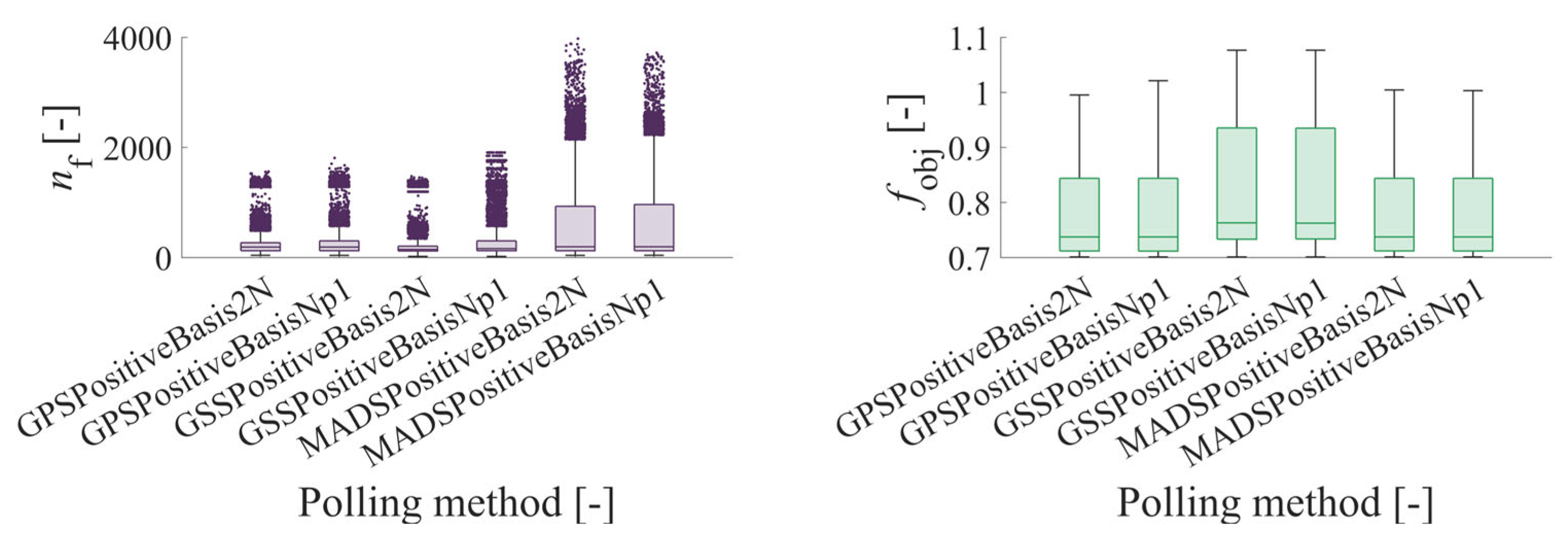
Figure 11.
The effect of the Polling method on the number of objective function evaluations and its value in the case of PSCH using the analytical solution of the journal bearing.
Figure 11.
The effect of the Polling method on the number of objective function evaluations and its value in the case of PSCH using the analytical solution of the journal bearing.
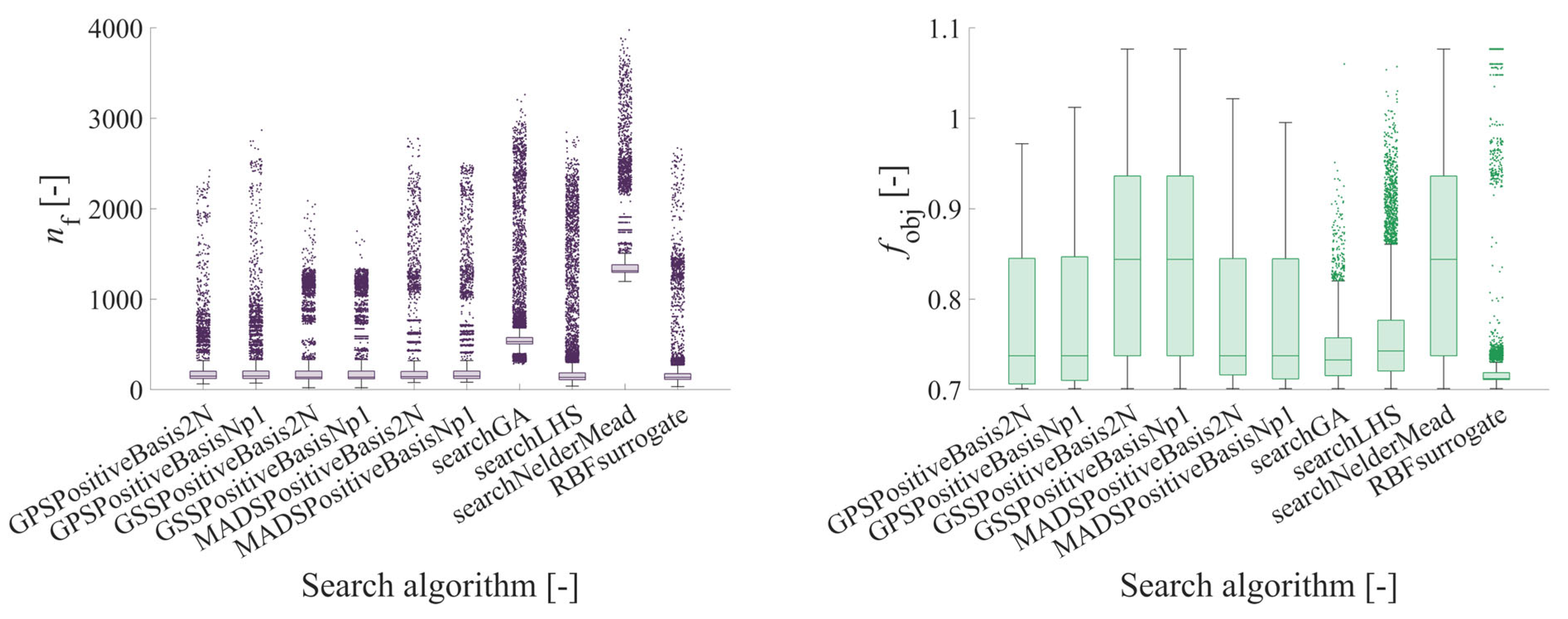
Figure 12.
The effect of the type of search algorithm on the number of objective function evaluations and its value in the case of PSCH using the analytical solution for the journal bearing.
Figure 12.
The effect of the type of search algorithm on the number of objective function evaluations and its value in the case of PSCH using the analytical solution for the journal bearing.
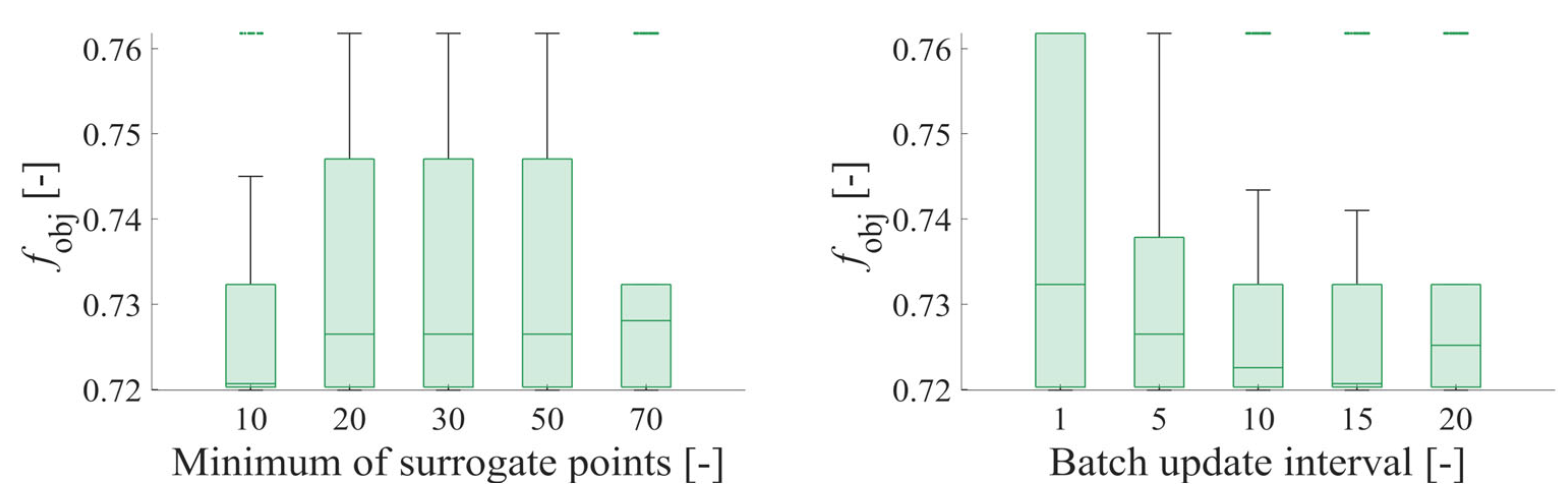
Figure 13.
Effect of the minimum of surrogate points and Batch update interval parameters on the number of objective function expressions in the SURG case using the analytical solution of the journal bearing.
Figure 13.
Effect of the minimum of surrogate points and Batch update interval parameters on the number of objective function expressions in the SURG case using the analytical solution of the journal bearing.
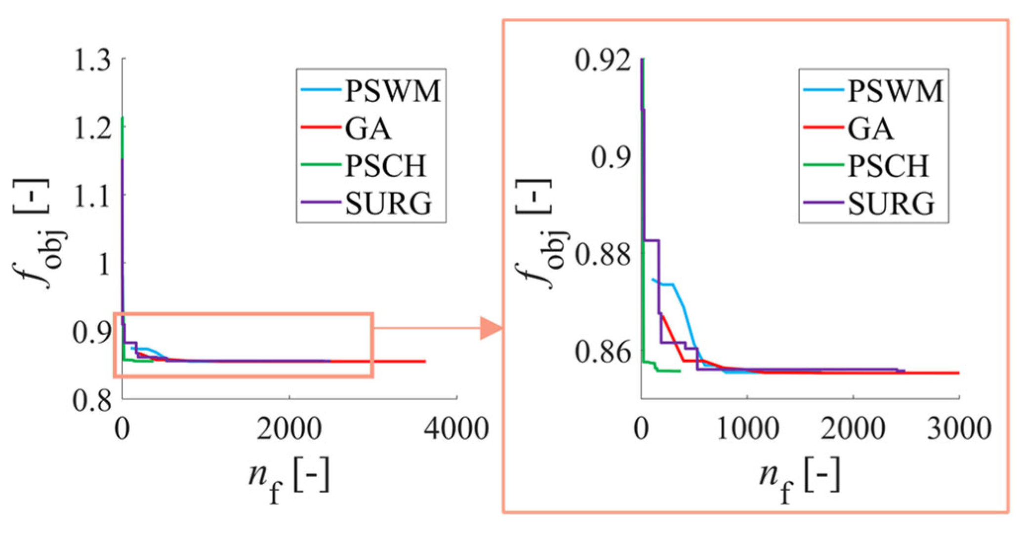
Figure 14.
Comparison of progression of objective function values for each optimisation algorithm, with detail (a) showing the region with minimal changes in (PSWM) and detail (b) showing the stagnation region of the search function (PSCH).
Figure 14.
Comparison of progression of objective function values for each optimisation algorithm, with detail (a) showing the region with minimal changes in (PSWM) and detail (b) showing the stagnation region of the search function (PSCH).
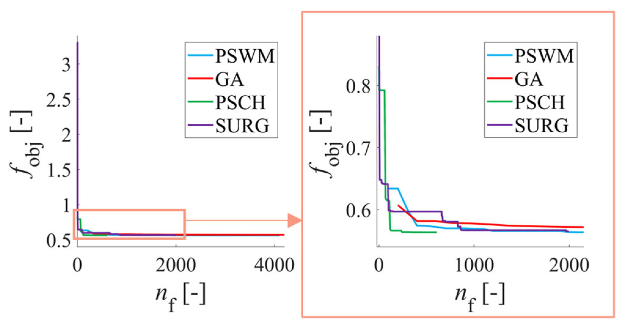
Figure 15.
Comparison of the objective function value progress for each optimisation algorithm in the optimisation of a journal bearing with three variables.
Figure 15.
Comparison of the objective function value progress for each optimisation algorithm in the optimisation of a journal bearing with three variables.
Figure 16.
Comparison of the progression of objective function values for individual optimisation algorithms in the case of optimising a thrust bearing with five variables.
Figure 16.
Comparison of the progression of objective function values for individual optimisation algorithms in the case of optimising a thrust bearing with five variables.
Table 1.
Journal bearing design parameters.
Table 1.
Journal bearing design parameters.
| Parameter | Value | Range |
|---|
| Bearing diameter, | 32 | 28–32 |
| Bearing width, | 17 | 13–17 |
| Bearing clearance, | 0.050 | 0.020–0.070 |
Table 2.
Thrust bearing design parameters. The values are valid for both the thrust and counter-thrust sides of the bearing.
Table 2.
Thrust bearing design parameters. The values are valid for both the thrust and counter-thrust sides of the bearing.
| Parameter | Value | Range |
|---|
| Number of pads, | 12 | – |
| Axial clearance, | 0.2 | – |
| Taper angle, [°] | 26 | |
| Wedge taper angle, | 0.2 | |
| Inner radius, | 75 | |
| Outer radius, | 130 | |
| Taper inner radius, | 77 | |
| Taper outer radius, | 128 | |
| Groove angular position, | 0 | |
| Groove heigh, | 0.5 | |
Table 3.
Hydrodynamic bearing operating conditions.
Table 3.
Hydrodynamic bearing operating conditions.
| Parameter | Value | | | |
|---|
| Operating condition no., | 1 | 2 | 3 | 4 |
| Rotor speed, | 5000 | 15,000 | 20,000 | 30,000 |
| Relative eccentricity, [–] | 0.32 | 0.24 | 0.3 | 0.21 |
| Radial pin velocity, m· | 0 | 0 | 0 | 0 |
| Oil temperature at inlet, | 60 | 60 | 60 | 60 |
| Dynamic viscosity, · | 0.005 | 0.005 | 0.005 | 0.005 |
| Oil density · | 840 | 840 | 840 | 840 |
| Oil heat capacity · | 2200 | 2200 | 2200 | 2200 |
| Load capacity limit of journal bearing | 100 | 100 | 150 | 150 |
| Mass flow rate limit of journal bearing · | 0.05 | 0.05 | 0.05 | 0.05 |
| Load capacity limit of thrust bearing | 250 | 480 | 670 | 1068 |
| Mass flow rate limit of thrust bearing · | 0.11 | 0.16 | 0.20 | 0.30 |
Table 4.
Algorithm settings used for PSWM.
Table 4.
Algorithm settings used for PSWM.
| Option | List of Tested Values and Options |
|---|
| Initial swarm span | 2000; 1000; 500; 3000; 5000; 10,000 |
| Minimum neighbours fraction | 0.25; 0; 0.5; 0.75 1 |
| Inertia range | 0.1–1.1; 0.1–2.1; 0.1–3.1 |
| Self adjustment weight | 1.49; 1.25; 1.75; 2 |
| Social adjustment weight | 1.49; 1.25; 1.75; 2 |
| Swarm size | 100 |
| Hybrid function | none; SQP [27,28,29,30]; Pattern search [31] |
| Function tolerance | |
| Max. Iterations | 600 |
| Max. Stall Iterations | 20 |
Table 5.
Algorithm settings used for GA.
Table 5.
Algorithm settings used for GA.
| Option | List of Tested Values and Options |
|---|
| Population size | 50; 100; 200; 500; 1000 |
| Fitness scaling | Rank fitness scaling [34]; top fitness scaling [34]; linear shift fitness scaling [34]; proportional fitness scaling; |
| Elite fraction | 0.05 |
| Crossover fraction | 0.7 |
| Crossover function | Laplace crossover [37]; heuristic crossover [38,39]; One-point crossover [40]; Two-point crossover [40]; Arithmetic crossover [41]; Scattered crossover [40] |
| Mutation function | Gaussian mutation [42]; mutationadaptfeasible [31]; Power mutation [39]; positive basis mutation [43] |
| Selection function | Tournament selection [44]; Remainder selection [44]; Roulette selection [44]; Uniform selection [44]; Stochastic universal selection [44] |
| Hybrid function | none; Pattern search [31]; SQP [27,28,29,30] |
| Max. Generations | 80 |
| Max. Stall Generations | 10 |
| Function tolerance | |
| Max. Stall Time | 300 |
Table 6.
Algorithm settings used for PSCH.
Table 6.
Algorithm settings used for PSCH.
| Option | List of Tested Values and Options |
|---|
| Algorithm | classic; NUPS [31,43,45,49]; NUPS-GPS [46,47,48]; NUPS-MADS [43] |
| Cache | on; off |
| Mesh rotate | on; off |
| Poll method | GPSPositiveBasis2 [31]; GPSPositiveBasisNp1 [31]; GSSPositiveBasis2N [46]; GSSPositiveBasisNp1 [46]; MADSPositiveBasis2N [49]; MADSPositiveBasisNp1 [49] |
| Search Function | GPSPositiveBasis2N [31]; GPSPositiveBasisNp1 [31]; GSSPositiveBasis2N [46]; GSSPositiveBasisNp1 [46]; MADSPositiveBasis2N [49]; MADSPositiveBasisNp1 [49]; searchGA [50]; searchLHS [51]; searchNelderMead [52]; RBFsurrogate [53,54,55] |
| Use complete poll | true; false |
| Use complete search | true; false |
| Poll order algorithm | Consecutive; Random; Success |
| Max. Iterations | 300 |
| Max. Function Evaluations | 6000 |
| Function Tolerance | |
| Step tolerance | |
| Mesh Tolerance | |
Table 7.
Algorithm settings used for SURG.
Table 7.
Algorithm settings used for SURG.
| Option | List of Tested Values and Options |
|---|
| Minimum surrogate points | 10; 20; 30; 50; 70 |
| Batch update interval | 1; 5; 10; 15; 20 |
| Maximum of function evaluations | 200; 500; 1000; 1500 |
Table 8.
Overview of the analysed number of settings for each algorithm without repetition to limit the initial seed of individuals.
Table 8.
Overview of the analysed number of settings for each algorithm without repetition to limit the initial seed of individuals.
| Function | Number of Variants |
|---|
| GA | 26,100 |
| PSWM | 4320 |
| PSCH | 11,328 |
| SURG | 100 |
| Total | 41,848 |
Table 9.
Efficiency evaluation for journal bearing optimisation using the analytical solution of the objective function for all algorithms and settings.
Table 9.
Efficiency evaluation for journal bearing optimisation using the analytical solution of the objective function for all algorithms and settings.
| Function | - | PSWM | GA | PSCH | SURG |
|---|
| Number of objective function evaluations, | Min | 746 | 570 | 20 | 195 |
| Max | 5160 | 77,554 | 3510 | 1500 |
| Mean | 1771 | 15,063 | 517 | 786 |
| Std | 470.47 | 16,849.00 | 507.85 | 493.97 |
| Objective function value, | Min | 0.7011 | 0.0098 | 0.7011 | 0.7199 |
| Max | 0.7026 | 0.9823 | 1.0766 | 0.7618 |
| Mean | 0.7011 | 0.7147 | 0.7958 | 0.7326 |
| Std | | 0.0267 | 0.0983 | 0.0161 |
Table 10.
Dependence of the objective function value and the number of its evaluations on the Cache and rotate mesh settings.
Table 10.
Dependence of the objective function value and the number of its evaluations on the Cache and rotate mesh settings.
| Setting | Cache | Rotate Mesh |
|---|
| | On | Off | On | Off |
|---|
| Median objective function value | 0.7374 | 0.7374 | 0.7374 | 0.7374 |
| Maximum of function evaluations—Q1 | 113 | 123 | 123 | 123 |
| Maximum of function evaluations—Q2 | 172 | 201 | 189 | 179 |
Table 11.
Effect of the poll ordering algorithm, complete poll and complete search on the number of objective function evaluations in the PSCH case using the analytical solution of the journal bearing.
Table 11.
Effect of the poll ordering algorithm, complete poll and complete search on the number of objective function evaluations in the PSCH case using the analytical solution of the journal bearing.
| Setting | Poll Ordering Algorithm | Complete Poll | Complete Search |
|---|
| | Random | Success | Consecutive | True | False | True | False |
|---|
| Median objective function value [] | 0.7374 | 0.7374 | 0.7374 | 0.7374 | 0.7374 | 0.7374 | 0.7374 |
| Maximum of function evaluations—Q1 | 123 | 123 | 123 | 123 | 123 | 123 | 123 |
| Maximum of function evaluations—Q2 | 186 | 184 | 179 | 190 | 177 | 189 | 176 |
| Maximum of function evaluations—Q3 | 501 | 501 | 501 | 503 | 500 | 505 | 499 |
Table 12.
Effect of the maximum of function evaluations parameter on the number of objective function expressions in the PSCH case using the analytical solution of the journal bearing.
Table 12.
Effect of the maximum of function evaluations parameter on the number of objective function expressions in the PSCH case using the analytical solution of the journal bearing.
| Maximum of function evaluations | 200 | 500 | 1000 | 1500 |
| Median objective function value | 0.7618 | 0.7323 | 0.7199 | 0.7206 |
Table 13.
The result efficient settings of PSWM.
Table 13.
The result efficient settings of PSWM.
| Option | Value |
|---|
| Initial swarm span | 500 |
| Minimum neighbours fraction | 0 |
| Inertia range | 0.1–1.1 |
| Self adjustment weight | 1.25 |
| Social adjustment weight | 1.49 |
| Swarm size | 100 |
| Hybrid function | SQP |
| Function tolerance | |
| Max. Iterations | 600 |
| Max. Stall Iterations | 20 |
Table 14.
The result efficient settings of GA.
Table 14.
The result efficient settings of GA.
| Option | Value |
|---|
| Population size | 1000 |
| Fitness scaling | Rank fitness scaling |
| Elite fraction | 0.05 |
| Crossover fraction | 0.7 |
| Crossover function | Heuristic crossover |
| Mutation function | Mutationadaptfeasible |
| Selection function | Remainder selection |
| Hybrid function | SQP |
| Max. Generations | 80 |
| Max. Stall Generations | 10 |
| Function tolerance | |
| Max. Stall Time | 300 |
Table 15.
The result efficient settings of PSCH, where is the number of design parameters used for optimisation.
Table 15.
The result efficient settings of PSCH, where is the number of design parameters used for optimisation.
| Option | Value |
|---|
| Algorithm | classic |
| Cache | on |
| Mesh rotate | on |
| Poll method | GPSPositiveBasis2N |
| Search function | MADSPositiveBasis2N |
| Use complete poll | false |
| Use complete search | true |
| Poll order algorithm | consecutive |
| Max. Iterations | |
| Max. Function Evaluations | |
| Function tolerance | |
| Step tolerance | |
| Mesh tolerance | |
Table 16.
The result efficient settings of SURG.
Table 16.
The result efficient settings of SURG.
| Option | Value |
|---|
| Minimum surrogate points | 70 |
| Batch update interval | 15 |
| Maximum of function evaluations | 1500 |
Table 17.
Results for all algorithms with optimal settings.
Table 17.
Results for all algorithms with optimal settings.
| Function | - | PSWM | GA | PSCH | SURG |
|---|
| Number of objective function evaluations | Min | 3977 | 20,141 | 142 | 1500 |
| Max | 7477 | 26,791 | 142 | 1500 |
| Mean | 5580 | 23,311 | 142 | 1500 |
| Std | 724.1141 | 1185.8935 | 0.0000 | 0.0000 |
| Objective function value | Min | 0.7011 | 0.7011 | 0.7011 | 0.7199 |
| Max | 0.7011 | 0.7011 | 0.7011 | 0.7199 |
| Mean | 0.7011 | 0.7011 | 0.7011 | 0.7199 |
| Std | | | | |


