Abstract
Firstly, the Reynolds equation considering gas inertia force is theoretically deduced in the cylindrical coordinate system, and then a mathematical model of aerostatic thrust bearing with three degrees of freedom (3-DOF) is constructed. Secondly, the Reynolds equation and velocity control equation are solved by the finite difference method (FDM), and the characteristics of gas pressure and velocity distribution in the gas film under steady-state conditions are revealed. On this basis, in the single-factor analysis, the bearing capacity error and recovery torque error caused by the inertia force term are quantitatively analyzed. It is found that the bearing rotating speed has a significant influence on the inertial force error, and the bearing radius also has a certain influence on the inertial force error, while the initial clearance, gas supply pressure, and torsion angle have relatively little influence on the inertial force error. Finally, in the multi-factor analysis, the sample regression equation of relative error of bearing capacity and relative error of restoring torque is established by using the multiple regression analysis method. By comparing the estimated values with the simulation results, the validity of the constructed regression equation is verified.
1. Introduction
Aerostatic bearing is widely used in various high-precision and high-speed equipment because of its advantages of high precision, high speed, low friction, and no pollution [1,2]. As the main component of ultra-precision machine tools, the performance of the aerostatic motorized spindle directly affects the surface quality and machining accuracy of the machined workpiece [3,4]. With the increasingly stringent requirements for the rotational speed and stability of the spindle in the product manufacturing process, the performance of the gas bearing also proposes higher requirements. Determining how to calculate the static and dynamic characteristics of gas bearing more accurately and establish a mathematical model more in line with the real working conditions is very important for the performance evaluation and structural design of the aerostatic motorized spindle [5]. In the previous numerical calculation of aerostatic bearing, gas inertia force, as a small factor affecting the performance of aerostatic bearing, is often ignored [6,7]. Under specific structural parameters and application conditions, ignoring the influence of inertia force may cause a large calculation error.
Relevant scholars have carried out some research on the influence of inertial force on the performance of gas bearings. Among them, Brand [8] concluded through dimensional analysis that when the corrected Reynolds number approaches or exceeds 1, the inertial force will have an important influence on aerostatic radial bearings. However, the research results presented by Gargiulo [9] indicated that even if the corrected Reynolds number reaches 1, the inertia correction coefficient of pressure distribution remains less than 0.3%, suggesting that the inertia force is still not a significant factor for gas bearings. Launder et al. [10,11] proposed two numerical calculation methods, which were, respectively, employed to calculate the laminar and turbulent inertial flow problems within the film of a finite-width thrust bearing. By comparing their findings with the results of various theories, the validity of the proposed methods was substantiated, and the significance of incorporating fluid inertial effects into lubrication analysis was underscored. Mori et al. [12,13] deduced the fluid control equation in the cylindrical coordinate system considering the gas extrusion effect and inertia force and studied the influence of inertia force on the gas velocity and pressure distribution characteristics in the solution domain of aerostatic thrust bearing. The results showed that the velocity distribution curve in the gas film changed from parabolic to elliptic function after considering the inertia force, which made the gas film pressure distribution change to some extent, but the bearing performance changed little. Hashimoto and Wada [14,15] studied the influence of turbulence and inertia force on the thrust bearing performance, and the results showed that under certain conditions, inertia force had a significant impact on the static characteristics of the bearing, and the theoretical calculation was verified by experimental results. Stolarski et al. [16] derived the Reynolds equation with the inertia term and used the concept of average inertia to deal with the inertia force in the thickness direction of the gas film, pointing out that the modified Reynolds equation was discretized by the control volume method, and at the same time, the convergence result of the gas film could be easily obtained by combining the Newton–Raphson iteration method. Yang [17] took the plane gas thrust bearing with spiral groove as the research object, solved the Reynolds equation with gas inertia force by finite element method, and studied the influence of bearing structure parameters on its bearing performance. Shen et al. [18] studied the influence of gas inertia effect and end face inclination on the steady and dynamic characteristics of ultra-high-speed spiral groove end face seal. The results showed that under ultra-high-speed conditions, the leakage rate of dry gas seal was significantly reduced and the rigid-leakage ratio was significantly increased, while the opening force, gas film stiffness, and dynamic characteristic coefficient changed little.
To sum up, although the existing literature includes research on the effect of inertia force on the performance of gas bearings, most of the work still stays in qualitative analysis, and even the results obtained in some research are contradictory, such as [8,9]. For different structural parameters, working parameters, and gas parameters of bearings, the quantitative analysis of the influence of inertia force on the performance of bearings is still quite lacking. In addition, some scholars [19,20] simplified the theoretical model in the previous research, ignoring the rotational freedom of the bearing, which made the model different from the real working state of the gas bearing. Therefore, aiming at the shortcomings of previous research, this paper takes aerostatic thrust bearing as the research object and obtains the Reynolds equation considering gas inertia force in the cylindrical coordinate system through theoretical derivation. At the same time, a 3-DOF gas film model of thrust bearing is established by fully considering the influence of bearing rotation freedom. The Reynolds equation and velocity control equation are solved by the FDM, and the pressure and velocity distribution of gas in the gas film considering the gas inertia force term are obtained. In addition, the influence of bearing initial clearance, radius, rotating speed, gas supply pressure, and torsion angle on bearing capacity error and recovery torque error caused by inertia force is quantitatively analyzed. On this basis, the sample regression equation of bearing capacity relative error and recovery torque relative error under the influence of multiple factors is obtained by using the method of multiple regression analysis, and the effectiveness of the equation is verified.
2. Mathematical Modeling
The structural schematic diagram of the aerostatic thrust bearing studied in this paper is shown in Figure 1. From the figure, it can be seen that the solution domain of the thrust bearing is circular, so the pressure and velocity distribution of gas in the gas film can be obtained by solving the fluid control equation in the cylindrical coordinate system.
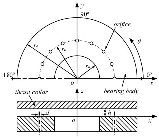
Figure 1.
Structural schematic diagram of the aerostatic thrust bearing.
2.1. Velocity Control Equation
According to the related literature [14], in the cylindrical coordinate system, the equation of motion considering the inertial force can be expressed as
By integrating z on both sides of the first equation and the second equation of Equation (1), Equation (2) can be obtained:
We introduce velocity boundary conditions:
And bring it into Equation (2) to obtain the velocity control equation of gas in the gas film:
Then, the average velocity equation of gas in the gas film can be expressed as
We introduce dimensionless parameters:
Substituting Equation (6) into Equation (4) and Equation (5), respectively, the dimensionless velocity equation and dimensionless average velocity equation can be obtained, as shown in Equations (7) and (8):
2.2. Reynolds Equation
In the cylindrical coordinate system, the continuous equation of gas in the gas film can be expressed as
where δi is the Kronecker function, which is 1 at the orifice nodes and 0 at the other nodes. By bringing Equation (4) into Equation (9), the general Reynolds equation in the cylindrical coordinate system can be obtained:
Meanwhile, dimensionless Equation (6) is brought into Equation (10) to obtain the dimensionless Reynolds Equation (11):
where the expressions of Q, Λ, and σ are
To facilitate the solution, the Reynolds equation in the cylindrical coordinate system is transformed by conformal transformation, so that the left end of the equation is transformed into the same form as that in the rectangular coordinate system. The conformal transformation equation is
By substituting Equation (13) into Equation (11), the dimensionless Reynolds equation after coordinate transformation can be obtained, as shown in Equation (14):
According to the method of the average inertia term mentioned in [14,16], the velocity term in Equation (14) is calculated by the average velocity in this paper.
2.3. Flow Control Equation
According to [21], the mass flow rate of gas entering the gas film from a single orifice can be expressed as follows:
where Φ is the mass flow coefficient, which is usually taken as 0.8.
In the process of using the aerostatic motorized spindle, when the spindle is subjected to external force, it will cause its translation and rotation in space, which will lead to a certain degree of inclination of the thrust collar in three-dimensional space.
Figure 2 shows the space attitude diagram of the thrust collar in an inclined state. In the frame of the coordinate system established in Figure 2, the gas film thickness of the thrust bearing can be expressed as
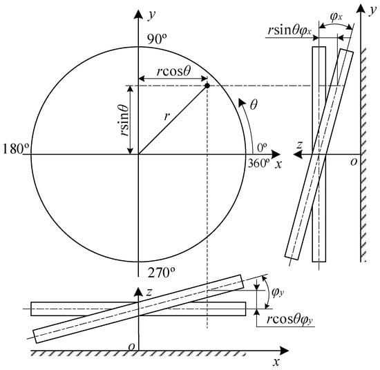
Figure 2.
Space attitude diagram of the thrust collar in an inclined state.
Its dimensionless form can be expressed as
By solving Equation (8) and Equation (14) jointly, the pressure value of each node in the solution domain can be obtained, and by integrating the pressure, the axial bearing capacity Fz, recovery torque Mx around the x-axis, and recovery torque My around the y-axis of thrust bearing can be obtained. The expressions are as follows:
3. Numerical Calculation and Verification
3.1. Numerical Calculation
The solution domain of aerostatic thrust bearing studied in this paper is circular. After the conformal transformation of coordinates by Equation (13), the solution domain of the thrust bearing is transformed into a rectangular region, as shown in Figure 3. Figure 3 contains three boundary types, namely, atmospheric boundary, orifice boundary, and symmetrical boundary. The boundary conditions on different boundaries are as follows:
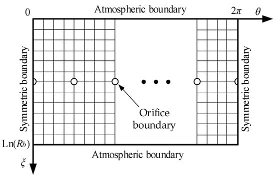
Figure 3.
Solution domain of the aerostatic thrust bearing.
Using the central difference scheme in the finite difference method to discretize Equations (8) and (14), their difference equations can be obtained, respectively, and the velocity and pressure of each node in the solution domain can be obtained by solving the difference equations through the successive overrelaxation method. Figure 4 shows the specific solution flow.
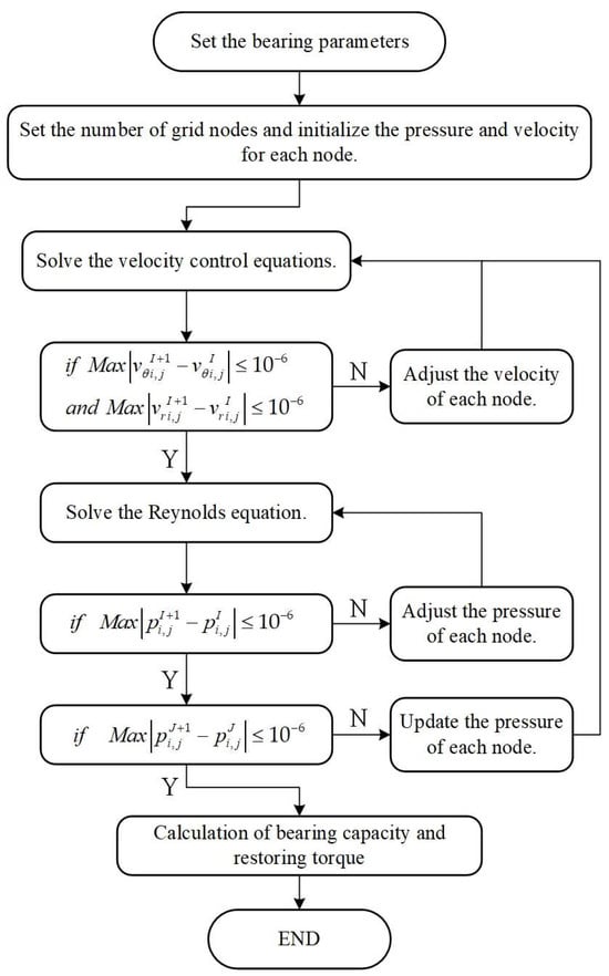
Figure 4.
Flow chart of the numerical solution.
3.2. Grid Independence Verification
In the process of numerical calculation, the number of grids is very important for the accuracy of the solution. Too few grids will lead to too much deviation between the simulation results and the exact solution, which cannot meet the requirements of the solution accuracy, while too many grids will lead to a too-long calculation time and reduce the solution efficiency. Therefore, it is necessary to verify the independence of grids to determine the necessary number of grids in the solution process. The main structural parameters and working parameters of the aerostatic thrust bearing studied in this paper are shown in Table 1.

Table 1.
Parameters of aerostatic thrust bearing.
When φx and φy are both 0, the bearing capacity value obtained by numerical calculation is used as the judgment basis to verify the irrelevance of the grid in the solution domain. The initial grid number nθ × nr is set to 80 × 15, and the grid refinement factor ng is the encryption multiple of the grid in a single direction. By densifying the grids in the solution domain, the bearing capacity obtained by numerical calculation gradually converges, as shown in Figure 5. Based on the final convergence result, when the relative error of bearing capacity Er reaches the preset error threshold of 2%, it is considered that the number of grids can meet the requirements of solution accuracy. According to Figure 5, it can be seen that when the grid refinement factor increases to 7, the relative error of bearing capacity is less than the established error threshold. Therefore, the final determined nθ × nr is 560 × 105.
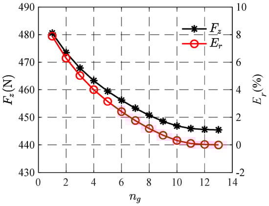
Figure 5.
Influence of the number of grids on the solution results.
3.3. Contrast Verification
To verify the correctness of the above solution process, the following is compared with the simulation results in the existing published literature. The simulation results obtained by the solution program used in this paper are compared with those obtained by Shi et al. in the published literature [22]. The structural parameters and working parameters of the bearing are shown in Table 2, and the comparison of the results is shown in Figure 6. When comparing Figure 6a,b, it can be seen that the pressure distribution curve obtained by the simulation program in this paper is consistent with the pressure distribution curve obtained in [22], and the numerical value is basically the same. Therefore, the validity of the solution program in this paper can be verified.
Table 2.
Bearing parameters in reference [22].
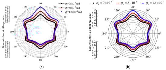
Figure 6.
Comparison between the simulation results in this paper and those in reference [22]. (a) Simulation results in reference [22]. (b) Simulation results obtained by solving the program in this paper.
4. Results and Analysis
4.1. Static Characteristics Analysis
In the actual working process of the aerostatic motorized spindle, the spindle will produce translation and rotation after being forced, which will change the spatial position of the thrust collar. This change will directly affect the gas film distribution of the thrust bearing and then have an important impact on the pressure and velocity distribution of gas in the gas film. The parameters of aerostatic thrust bearings studied in this paper are shown in Table 1. When the values of φx and φy are both 2 × 10⁻⁴ rad, the gas pressure distribution in the gas film obtained by the numerical solution is shown in Figure 7, and the circumferential average velocity distribution and the radial average velocity distribution of the gas in the film are shown in Figure 8 and Figure 9, respectively.
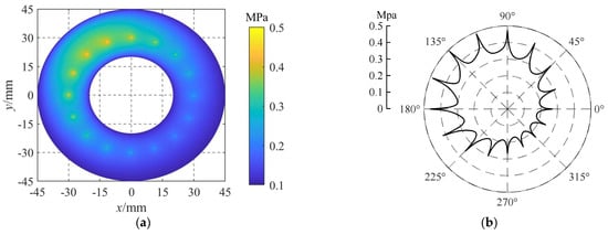
Figure 7.
Gas pressure distribution in the gas film. (a) Gas film pressure distribution cloud map. (b) Pressure distribution curve at the orifice distribution circle.
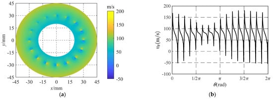
Figure 8.
Circumferential average velocity distribution of gas in the gas film. (a) Circumferential average velocity distribution cloud map. (b) Circumferential average velocity distribution curve at the orifice distribution circle.
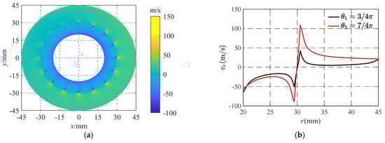
Figure 9.
Radial average velocity distribution of gas in the gas film. (a) Radial average velocity distribution cloud map. (b) Radial average velocity distribution curve at a specific position.
As can be seen from Figure 7a, the torsion angle of the thrust collar will seriously affect the pressure distribution of gas in the gas film. Because the torsion angles of the thrust collar on the x-axis and the y-axis are both positive values, the gas film thickness is the smallest at θ = 3/4π, and the gas film pressure near this angle is the largest, while the gas film thickness at θ = 7/4π is the largest and the gas film pressure near this angle is the smallest. In addition, because the rotation direction of the thrust collar is counterclockwise, under the influence of the dynamic pressure effect, the high-pressure region in the gas film will shift to a certain extent in the direction of smaller θ. As shown in Figure 7b, under the same gas supply pressure, the pressure behind the orifice at θ = 3/4π is close to 0.5 Mpa, while the pressure behind the orifice at θ = 7/4π is only about 0.25 Mpa. This shows that the film thickness at the orifice has a significant influence on the pressure behind the orifice. Specifically, the smaller the film thickness at the orifice, the greater the pressure, and vice versa.
As shown in Figure 8a, with the increase in the gas film radius, the circumferential average velocity of gas in the gas film shows a trend of increasing gradually. At the orifice node, because the high-pressure gas flows into the gas film through the orifice, it will quickly spread around, which leads to a significant increase in the gas velocity gradient near the orifice, thus causing an obvious sudden change in the circumferential average velocity. In addition, combined with Figure 8b, it can be further observed that there is a positive correlation between the velocity variation amplitude at the orifice and the film thickness. Specifically, at θ = 3/4π, the film thickness is the smallest, and the velocity variation amplitude is also the smallest. At θ = 7/4π, the film thickness is the largest, and the velocity variation amplitude is also the largest. This phenomenon shows that the film thickness has an important influence on the gas flow characteristics.
As shown in Figure 9a, the radial average velocity of gas is different under different angular coordinates. Generally speaking, the change amplitude of the radial average velocity of the gas is relatively small near θ = 3/4π, but it increases significantly near θ = 7/4π. In addition, it can be observed from the figure that the radial average velocity of the gas in the gas film changes in the flow direction at the orifice distribution circle. The concrete manifestations are as follows: for the nodes whose radial coordinates are greater than the radius of the distribution circle, the radial velocity is positive, indicating that the gas flows outward; for the nodes whose radial coordinates are smaller than the radius of the distribution circle, the radial velocity is negative, indicating that the gas flows inward. Figure 9b further shows the distribution characteristics of gas radial average velocity along radial coordinates at θ1 = 3/4π and θ2 = 7/4π. It can be seen that the radial average velocity suddenly changes at r = 30 mm due to the diffusion of gas into the gas film, and the suddenly changed velocity values are located on both sides of the 0 velocity line. By comparing the radial velocity curves at θ1 and θ2, it can be found that the radial average velocity at θ1 is lower than that at θ2, which indicates that the radial velocity distribution of gas is also positively correlated with the bearing gas film thickness.
Combined with the analysis results of Figure 7, Figure 8 and Figure 9, it can be seen that the torsion angle of the thrust collar has a significant influence on the pressure distribution and velocity distribution of the aerostatic thrust bearing. Therefore, in the simulation calculation, the influence of the rotational degree of freedom of the thrust collar on the gas flow characteristics must be fully considered.
4.2. Single-Factor Analysis of Inertial Force Error
In the analysis of aerostatic bearings, the gas inertial force is considered to describe the flow behavior of gas in the bearing gap more accurately, especially at high speed or acceleration. The introduction of inertial force will increase the complexity of the model, but it can reflect the dynamic characteristics of the fluid more truly, thus improving the accuracy and reliability of the analysis. According to the description in [21], the influence of gas inertia force on the performance of aerostatic bearing can be roughly evaluated by multiplying the gas Reynolds number in the gas film by the ratio of gas film thickness to bearing radius, and its expression is
Although this evaluation method cannot accurately calculate the size of bearing performance error caused by inertial force term, it can be seen from its expression that the size of inertial force error is mainly related to key parameters such as gas density, velocity, gas film thickness, and bearing geometry size. Among them, the gas density and velocity are mainly determined by the gas supply pressure and rotating speed, while the gas film thickness is influenced by the initial clearance of the bearing and the torsion angle of the thrust collar. Therefore, the gas supply pressure, rotational speed, gas film thickness, torsion angle, and bearing radius are the main influencing factors in this paper, and we quantitatively study the influence of inertia force term on bearing performance.
The relative error of bearing performance caused by gas inertia force term can be expressed as
4.2.1. Influence of Initial Clearance on Inertial Force Error
For aerostatic bearings, the gas film thickness has a very important influence on the performance of bearings. When the value of φx is 1 × 10⁻⁴ rad and the value of φy is 0, other parameters are shown in Table 1. The curves of axial bearing capacity Fz and torque around the x-axis Mx with the initial clearance obtained by numerical calculation are shown in Figure 10a. The curves of the relative error of bearing capacity EFz and the relative error of torque around the x-axis EMx caused by inertia force with the initial clearance are shown in Figure 10b.
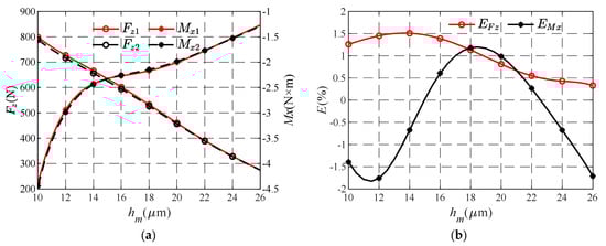
Figure 10.
The performance parameters and their relative errors vary with the initial clearance. (a) Variation curve of Fz and Mx with hm. (b) Variation curve of EFz and EMx with hm.
As can be seen from Figure 10a, with the increase in initial clearance, the axial bearing capacity Fz gradually decreases, and the value of Fz1 is always slightly larger than Fz2, but the gap between them gradually becomes smaller and tends to overlap. Observing the change curve of torque around the x-axis Mx, it can be found that because φx is positive, the thrust bearing will produce recovery torque that makes the thrust collar rotate around the x-axis in the opposite direction, so the torque produced by the thrust bearing is negative. At the same time, observing the change of torque, it can be found that with the increase in initial clearance, the recovery torque produced by the thrust bearing decreases gradually, and the reduction rate of Mx is faster when the initial clearance is less than 14 μm, slower when the initial clearance is between 14 μm and 20 μm and increases again when the initial clearance is greater than 20 μm, and decreases linearly. When comparing the two curves of Mx1 and Mx2, it can be seen that the two curves corresponding to Mx1 and Mx2 basically coincide, which shows that the inertia force error caused by the change of bearing initial clearance is not large.
As can be seen from Figure 10b, with the change in initial clearance, the overall EFz curve shows a decreasing trend. When the initial clearance is 14 μm, the EFz reaches the maximum value, which is about 1.5%. At the same time, the EMx curve fluctuates in a certain range with the change in initial clearance, but the fluctuation amplitude of its relative error never exceeds 2%. The comprehensive evaluation of the influence of initial clearance on EFz and EMx curves shows that the change in initial clearance has a relatively small influence on the inertial force error, which does not exceed the preset error threshold of 2%.
4.2.2. Influence of Bearing Radius on Inertial Force Error
The size of the bearing will affect the Reynolds number of the gas in the gas film. When the difference between the inner and outer radius of the bearing is constant, the outer radius rb of the bearing increases from 35 mm to 80 mm. The curves of Fz and Mx with the bearing radius are shown in Figure 11a, and the curves of EFz and EMx with the bearing radius are shown in Figure 11b.
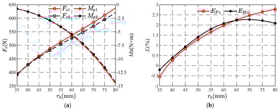
Figure 11.
The performance parameters and their relative errors vary with the bearing radius. (a) Variation curve of Fz and Mx with rb. (b) Variation curve of EFz and EMx with rb.
Figure 11a reveals the influence of bearing radius on Fz and Mx performance parameters. Specifically, with the increase in bearing radius, the Fz curve shows a nearly linear growth trend. By further comparing the Fz1 and Fz2 curves, it can be found that when the bearing radius is small, they almost coincide, but as the bearing radius increases, the gap between them gradually expands. When observing the change law of the Mx curve, it can be seen that Mx increases with the increase in bearing radius, and the growth rate is gradually accelerated. When comparing the two curves of Mx1 and Mx2, it can be found that the variation rules of the two curves are the same and the numerical differences are small. However, as the bearing radius increases, the absolute error between them also gradually becomes obvious. The main reason for the above changes is that with the increase in bearing size, not only does the bearing area of the gas bearing increase but the bearing is also affected by the dynamic pressure effect, resulting in a significant increase in bearing capacity and recovery torque. In addition, the increase in bearing radius leads to the increase in Reynolds number of gas in the gas film, and then the absolute error of bearing performance parameters caused by inertial force term increases gradually. Therefore, the curve difference between ignoring inertia force and considering inertia force is gradually obvious.
In Figure 11b, the value of EFz increases with the increase in bearing radius, but the growth rate gradually decreases. When the bearing radius is greater than 60 mm, the value of EFz will be greater than 2%. It can be seen that the relative error of bearing capacity caused by inertia force is already large. With the increase in bearing radius, EMx first increases and then decreases. When the outer radius of the bearing is 65 mm, EMx reaches the maximum value, which is about 2.2%, and when the radius of the bearing outer circle is between 60 mm and 80 mm, the values of EMx all exceed 2%. The comprehensive analysis in Figure 11 shows that the bearing size has a great influence on the inertial force error, and the larger the bearing size, the greater the error caused by the inertial force term.
4.2.3. Influence of Rotating Speed on Inertial Force Error
The bearing rotating speed has a great influence on the Reynolds number of the gas in the gas film. When the rotating speed gradually increases from 40,000 rpm to 140,000 rpm, the curves of Fz and Mx with the rotating speed are shown in Figure 12a, and the curves of EFz and EMx with the rotating speed are shown in Figure 12b.
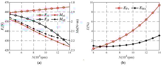
Figure 12.
The performance parameters and their relative errors vary with the rotating speed. (a) Variation curve of Fz and Mx with N. (b) Variation curve of EFz and EMx with N.
As can be seen from Figure 12a, there is a very obvious difference between the two curves corresponding to Fz1 and Fz2. Specifically, with the increase in rotational speed, the value of Fz1 is always greater than the value of Fz2, Fz1 increases slowly in a straight line, while Fz2 shows a downward trend, and the rate of decline gradually accelerates. When comparing the two curves of Mx1 and Mx2, it can be seen that the values of Mx1 and Mx2 increase with the increase in rotational speed, and in the process of change, Mx1 is always greater than Mx2. In addition, the Mx1 curve almost grows linearly, while the growth rate of the corresponding curve of Mx2 gradually slows down. This paper holds that the main reason for this difference is that when the bearing speed is high, the bearing is greatly influenced by the inertial force term, which makes the dynamic characteristics of gas flow more complicated. The change in gas flow characteristics will change the distribution of gas pressure to a certain extent, resulting in uneven distribution of gas film pressure, thus reducing the bearing capacity and having a certain impact on the recovery torque of the bearing.
Figure 12b shows the changes of EFz and EMx with the rotating speed. It can be seen that both curves increase with the increase in rotating speed. Among them, the growth rate of the EFz curve is relatively fast, and with the increase in rotational speed, the growth rate gradually accelerates. When the rotational speed exceeds 7 × 10⁴ rpm, the EFz value will exceed 2%, indicating that the inertial force has a great influence on the bearing capacity error. In contrast, the growth rate of the EMx curve is relatively small. When the rotation speed is less than 8 × 10⁴ rpm, the EMx value is relatively stable and remains at about 1%. However, as the rotation speed continues to increase, the growth rate of the EMx curve gradually accelerates, and when the rotation speed is greater than 12 × 104 rpm, the value exceeds 2%. Through the influence of the inertial force on the bearing capacity and torque of the gas bearing, it can be seen that the bearing speed has a significant effect on the inertial force error. Therefore, when the bearing speed is high, the influence of the inertial force term cannot be ignored.
4.2.4. Influence of Gas Supply Pressure on Inertial Force Error
The gas supply pressure will affect the pressure and velocity distribution of gas in the gas film. When the gas supply pressure is increased from 0.3 Mpa to 0.7 Mpa, the curves of Fz and Mx with the gas supply pressure are shown in Figure 13a, and the curves of EFz and EMx with the gas supply pressure are shown in Figure 13b.
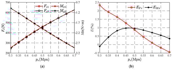
Figure 13.
The performance parameters and their relative errors vary with gas supply pressure. (a) Variation curve of Fz and Mx with ps. (b) Variation curve of EFz and EMx with ps.
In Figure 13a, both Fz and Mx increase linearly with the increase in gas supply pressure. It can be seen that there is only a small difference between the bearing capacity and torque under the condition of considering inertia force and not considering inertia force, indicating that the influence of inertia force term on bearing performance is always small in the process of bearing gas supply pressure change. As can be seen from Figure 13b, the EFz curve decreases continuously with the increase in gas supply pressure. When the gas supply pressure is 0.3 Mpa, the value of EFz is the largest, but it is still less than 2.5%. When the gas supply pressure exceeds 0.6 Mpa, EFz even appears negative, indicating that when the gas supply pressure of the bearing is large enough, the bearing capacity under the condition of considering the gas inertia force is slightly larger than that without considering the inertia force. At the same time, it can be seen from the curve of EMx that with the increase in gas supply pressure, EMx first increases and then gradually decreases. When the gas supply pressure is 0.45 Mpa, EMx reaches the maximum value, but it still does not exceed 1%. According to the influence of inertia force on the absolute error and relative error of bearing capacity and torque under different gas supply pressures, it can be seen that the change in gas supply pressure has little influence on inertia force and very limited influence on bearing performance.
4.2.5. Influence of Torsion Angle on Inertial Force Error
The spatial attitude of the thrust collar will directly affect the gas film thickness distribution of the bearing, and it will also affect the pressure and velocity distribution of the gas in the gas film to a certain extent, thus affecting the magnitude of the inertia force term. With the torsion angle of the thrust collar as a variable, when the torsion angle φx increases from 0 to 2.5 × 10⁻⁴ rad, the curves of Fz and Mx with torsion angle are shown in Figure 14a, and the curves of EFz and EMx with torsion angle are shown in Figure 14b.
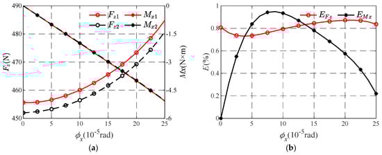
Figure 14.
The performance parameters and their relative errors vary with torsion angle. (a) Variation curve of Fz and Mx with φx. (b) Variation curve of EFz and EMx with φx.
As can be seen from Figure 14a, with the increase in the torsion angle of the thrust collar, the bearing capacity Fz gradually increases, and its growth rate also gradually increases. When comparing the two curves of Fz1 and Fz2, it can be seen that the value of Fz1 is always greater than Fz2 in the process of torsion angle change, and the absolute error between them has little change. It can be seen that the bearing capacity decreases after increasing the influence of the inertia force term, and in the process of torsion angle change, the change in bearing capacity error caused by inertial force is small. When observing the change curve of Mx, it can be found that with the increase in torsion angle, the value of Mx increases rapidly along the straight line, and the two curves of Mx1 and Mx2 almost coincide, indicating that the absolute error between the two is very small. As can be seen from Figure 14b, with the increase in torsion angle, the value of EFz is stable at about 0.8%, while the value of EMx increases first and then decreases gradually. When the torsion angle is 7.5 × 10⁻⁵ rad, EMx reaches the maximum value, but its maximum value is still less than 1%. It can be seen that the inertia force error caused by the torsion angle of the thrust collar is very limited. When considering the influence of gas inertia force on the absolute error and relative error of bearing capacity and torque under different torsion angles, it can be concluded that the change of torsion angle has little influence on the inertia force term.
4.3. Multiple Regression Analysis of Relative Error
From the above single-factor simulation results, it can be seen that the errors of bearing capacity and torque caused by gas inertia force are influenced by multiple factors. To evaluate the relative errors of bearing capacity and torque caused by inertia force under the joint influence of different structural parameters and working parameters, taking the above single-factor simulation results as samples, the first 9 simulation results of each group are taken to form a database of 45 units. Through regression analysis, the sample regression equation of the relative error of bearing capacity and the relative error of torque under the influence of multiple factors is obtained, and the validity of the regression equation is verified.
4.3.1. Establishment of Regression Equation
Figure 15 shows the values of each factor in 45 samples and the relative errors corresponding to each sample. According to the different linear relationship between the relative error of bearing capacity and various factors, and the different linear relationship between the relative error of recovery torque and various factors, the regression model is shown in Equation (23):
where eFz and eMx are estimated values of EFz and EMx, respectively; a0~a13 are the regression coefficient of eFz, and b0~b14 are the regression coefficient of eMx.
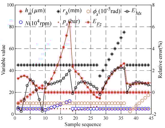
Figure 15.
The value of each factor in the sample library and the relative error of each sample.
Through the multiple regression analysis of the results in the sample database, and expressed in the above form, the specific values of each regression coefficient can be obtained. The sample regression equation finally obtained by calculation is shown in Equation (23), and the corresponding goodness of fits are 0.999 and 0.997, respectively. At the same time, as can be seen from Figure 16, the relative error value calculated by the sample regression equation is very consistent with the numerical calculation results, which reflects the rationality of the regression model.
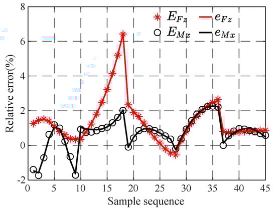
Figure 16.
Comparison chart of estimated value and simulation value.
4.3.2. Validation of Regression Equation
To verify the validity of the regression equation, six groups of bearing parameters were selected as verification samples. The accuracy and reliability of the sample regression equation were evaluated by comparing the relative error estimated by the regression equation with the numerical simulation results; see Table 3 for the specific values of the relevant independent variables in the verification sample.
Table 3.
Values of variables in validation samples.
It can be seen from Figure 17 that the curves of eFz and eMx calculated by the sample regression equation are basically the same as the corresponding curves of eFz and eMx calculated by numerical calculation., but there are still some differences in values, and the results calculated by sample regression equation are generally smaller than those calculated by numerical calculation. The main reason for the above differences is that the number of samples in the process of solving the regression equation is small, which leads to a certain deviation between the calculation results of the regression equation and the numerical calculation results. When comparing the two curves of EFz and eFz, it can be seen that the biggest difference between them appears in the fourth group of samples, and the difference is about 5%. At the same time, when observing EMx and eMx curves, we can see that the biggest difference between them appears in the third group of samples, and the difference is about 3%. It can be seen that although there are some differences between the relative error of regression analysis and numerical calculation, the error between them is not large, which can explain the effectiveness of the sample regression equation.
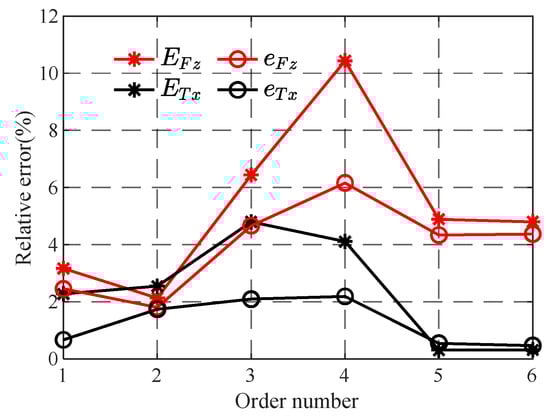
Figure 17.
Comparison chart of estimated value and simulation value of verification sample.
5. Conclusions
In this paper, firstly, the Reynolds equation in the cylindrical coordinate system was derived theoretically, and a mathematical model of 3-DOF aerostatic thrust bearing was established under the condition of fully considering the rotational freedom of the bearing. Secondly, the finite difference method was used to numerically calculate the bearing in the inclined state of the thrust collar, and the pressure and velocity distribution characteristics of the gas in the gas film under a steady state were obtained. In the single-factor analysis, the effects of initial clearance, radius, rotational speed, gas supply pressure, and torsion angle on the bearing capacity and recovery torque were studied. Finally, using the method of multiple regression analysis, the sample regression equations of relative error of bearing capacity and relative error of restoring torque were obtained, and the effectiveness of the regression equations was verified by simulation results. The main conclusions of this study are as follows:
- (1)
- The degree of freedom of bearing rotation will seriously affect the thickness distribution of the gas film, and then change the pressure and velocity distribution characteristics of gas in the gas film. At the same time, the smaller the film thickness, the greater the pressure, and the smaller the circumferential and meridional velocity changes at this position.
- (2)
- In single-factor analysis, it was found that the inertia force error caused by the change of bearing speed is the largest, and when the rotating speed exceeds 7 × 10⁴ rpm, the bearing capacity error will exceed 2%. The bearing radius also has a certain influence on the inertial force error; when it exceeds 60 mm, the relative error of the bearing capacity and the error of the recovery torque will exceed 2%. In addition, the research shows that the inertia force error caused by changing the bearing initial clearance, gas supply pressure, and torsion angle is small.
- (3)
- The sample regression equations of relative error of bearing capacity and relative error of torque were obtained by multiple regression analysis, and the estimated value of relative error obtained by verifying the regression equation in the sample was compared with the simulation value. The results show that the variation law of the estimated value and the simulation value is the same, and there are some differences in numerical values, but the error range is small, which can prove the effectiveness of the sample regression equation.
Author Contributions
Conceptualization, C.J. and S.J.; methodology, S.J.; software, S.J. and Y.L.; validation, C.J.; formal analysis, S.J.; investigation, Y.L. and S.J.; data curation, Y.L.; writing—original draft preparation, S.J.; writing—review and editing, S.J.; visualization, Y.L. and S.J.; funding acquisition, C.J. All authors have read and agreed to the published version of the manuscript.
Funding
This research was funded by the National Key Research and Development Program of China, grant number 2022YFB3402704.
Data Availability Statement
The data presented in this study are available on reasonable request from the corresponding author.
Conflicts of Interest
The authors declare no conflicts of interest.
Nomenclature
| r, θ, z | Coordinates |
| ra | Internal radius |
| rb | External radius |
| rc | Distribution circle radius |
| d | Orifice diameter |
| p | Gas film pressure |
| ρ | Gas density |
| η | Gas dynamic viscosity |
| t | Time |
| vr, vθ | Velocity |
| h | Gas film thickness |
| vra, vθa | Average velocity |
| l, p0, vm | Reference quantities of length, pressure, and speed |
| hm | Initial clearance |
| R, Z | Dimensionless coordinates |
| P | Dimensionless gas film pressure |
| H | Dimensionless gas film thickness |
| Vr, Vθ | Dimensionless velocity |
| T | Dimensionless time |
| w | Gas velocity flowing into the gas film from the orifice |
| δi | Kronecker function |
| pa | Atmospheric pressure |
| ρa | Gas density under atmospheric pressure |
| m | Mass flow of a single orifice |
| A | Orifice area |
| ps | Supply pressure |
| Φ | Mass flow coefficient |
| ψ | Flow function |
| k | Ratio of specific heat |
| β | Pressure ratio at the orifice |
| pd | Pressure at the orifice |
| βk | Critical pressure ratio |
| n | Orifice number |
| N | Rotating speed |
| nθ, nr | Grid number |
| ng | Grid refinement factor |
| φx, φy | Torsion angle |
| EFz, EMx, EMy | Relative error of bearing capacity and torque |
| Fz1, Mx1, My1 | Bearing capacity and torque when inertia force is ignored |
| Fz2, Mx2, My2 | Bearing capacity and torque when inertia force is considered |
References
- Gao, Q.; Chen, W.; Lu, L.; Huo, D.; Cheng, K. Aerostatic bearings design and analysis with the application to precision engineering: State-of-the-art and future perspectives. Tribol. Int. 2019, 135, 1–17. [Google Scholar] [CrossRef]
- Chen, G.; Ju, B.; Fang, H.; Chen, Y.; Yu, N.; Wan, Y. Air bearing: Academic insights and trend analysis. Int. J. Adv. Manuf. Tech. 2019, 106, 1191–1202. [Google Scholar] [CrossRef]
- Zhang, S.; Yu, J.; To, S.; Xiong, Z. A theoretical and experimental study of spindle imbalance induced forced vibration and its effect on surface generation in diamond turning. Int. J. Mach. Tool. Manu 2018, 133, 61–71. [Google Scholar] [CrossRef]
- Chen, D.J.; Huo, C.; Cui, X.X.; Pan, R.; Fan, J.W.; An, C.H. Investigation the gas film in micro scale induced error on the performance of the aerostatic spindle in ultra-precision machining. Mech. Syst. Signal Proc. 2018, 105, 488–501. [Google Scholar] [CrossRef]
- Wen, Z.P.; Gu, H.; Shi, Z.Y. Key Technologies and Design Methods of Ultra-Precision Aerostatic Bearings. Lubricants 2023, 11, 315–327. [Google Scholar] [CrossRef]
- Chen, G.D.; Chen, Y.J. Multi-Field Coupling Dynamics Modeling of Aerostatic Spindle. Micromachines 2021, 12, 251. [Google Scholar] [CrossRef] [PubMed]
- Lo, C.-Y.; Wang, C.-C.; Lee, Y.-H. Performance analysis of high-speed spindle aerostatic bearings. Tribol. Int. 2005, 38, 5–14. [Google Scholar] [CrossRef]
- Brand, R.S. Inertia Forces in Lubricating Films. J. Appl. Mech. 1955, 77, 363–364. [Google Scholar] [CrossRef]
- Gargiulo, E.P., Jr. A Re-Evaluation of Inertia Effects In Hydrodynamic Gas Journal Bearings. J. Lubr. Technol. 1976, 98, 187–188. [Google Scholar] [CrossRef]
- Launder, B.E.; Leschziner, M.A. Flow in Finite-Width, Thrust Bearings Including Inertial Effects: I—Laminar Flow. J. Lubr. Technol. 1978, 100, 330–338. [Google Scholar] [CrossRef]
- Launder, B.E.; Leschziner, M.A. Flow in Finite-Width Thrust Bearings Including Inertial Effects: II—Turbulent Flow. J. Lubr. Technol. 1978, 100, 339–345. [Google Scholar] [CrossRef]
- Mori, H. A theory of an externally pressurized circular thrust gas bearing with consideration of the effects of lubricant inertia. J. Basic. Eng. 1963, 85, 304–309. [Google Scholar] [CrossRef]
- Mori, A.; Tanaka, K.; Mori, H. Effects of Fluid Inertia Forces on the Performance of a Plane Inclined Sector Pad for an Annular Thrust Bearing Under Laminar Condition. J. Tribol. 1985, 107, 46–52. [Google Scholar] [CrossRef]
- Hashimoto, H. The effects of fluid inertia forces on the static characteristics of sector-shaped, high-speed thrust bearings in turbulent flow regime. J. Tribol. 1989, 111, 406–412. [Google Scholar] [CrossRef]
- Hashimoto, H.; Wada, S. Turbulent Lubrication of Tilting-Pad Thrust Bearings With Thermal and Elastic Deformations. J. Tribol. 1985, 107, 82–86. [Google Scholar] [CrossRef]
- Stolarski, T.A.; Chai, W. Inertia effect in squeeze film air contact. Tribol. Int. 2008, 41, 716–723. [Google Scholar] [CrossRef]
- Yang, X. Research on Bearing Performanceof High Speed Gas Thrust Bearing Withspiral Groove Under the Condition of Inertia Force; Harbin Institute of Technology: Harbin, China, 2017. [Google Scholar]
- Shen, W.; Peng, X.; Jiang, J.; Li, J.; Zhao, W. The Influence of Inertia Effect on Steady Performance and Dynamic Characteristic of Super High-Speed Tilted Gas Face Seal. Tribology 2019, 39, 452–462. [Google Scholar] [CrossRef]
- Zhuang, H.; Ding, J.; Chen, P.; Chang, Y.; Zeng, X.; Yang, H.; Liu, X.; Wei, W. Effect of Surface Waviness on the Performances of an Aerostatic Thrust Bearing with Orifice-Type Restrictor. Int. J. Precis. Eng. Manuf. 2021, 22, 1735–1759. [Google Scholar] [CrossRef]
- Cui, H.; Wang, Y.; Yue, X.; Li, Y.; Jiang, Z. Numerical analysis of the dynamic performance of aerostatic thrust bearings with different restrictors. Proc. Inst. Mech. Eng. Part J J. Eng. Tribol. 2018, 233, 406–423. [Google Scholar] [CrossRef]
- Liu, T.; Liu, Y.; Chen, S. Aerostatic Lubrication; Harbin Institute of Technology Press: Harbin, China, 1990. [Google Scholar]
- Shi, J.; Cao, H.; Chen, X. Effect of angular misalignment on the dynamic characteristics of externally pressurized air journal bearing. Proc. Inst. Mech. Eng. Part. J.-J. Eng. Tribol. 2019, 234, 205–228. [Google Scholar] [CrossRef]
Disclaimer/Publisher’s Note: The statements, opinions and data contained in all publications are solely those of the individual author(s) and contributor(s) and not of MDPI and/or the editor(s). MDPI and/or the editor(s) disclaim responsibility for any injury to people or property resulting from any ideas, methods, instructions or products referred to in the content. |
© 2025 by the authors. Licensee MDPI, Basel, Switzerland. This article is an open access article distributed under the terms and conditions of the Creative Commons Attribution (CC BY) license (https://creativecommons.org/licenses/by/4.0/).