Article

RUL Prediction of Rolling Bearings Based on Fruit Fly Optimization Algorithm Optimized CNN-LSTM Neural Network

1
School of Energy, Environment and Safety Engineering, China Jiliang University, Hangzhou 310018, China
2
Zhejiang Academy of Special Equipment Science, Hangzhou 310009, China
3
Taizhou Special Equipment Inspection and Testing Research Institute, Taizhou 318000, China
*
Author to whom correspondence should be addressed.
Lubricants 2025, 13(2), 81; https://doi.org/10.3390/lubricants13020081
Submission received: 18 December 2024 / Revised: 3 February 2025 / Accepted: 5 February 2025 / Published: 12 February 2025
(This article belongs to the Special Issue New Horizons in Machine Learning Applications for Tribology)

Abstract

:
Due to the complex changes in the physical and chemical properties of rolling bearings from degradation to failure, most model-driven and data-driven methods generally suffer from insufficient accuracy and robustness in predicting the remaining useful life of rolling bearings. To address this challenge, this paper proposes a data-driven artificial neural network method, namely the CNN-LSTM bearing remaining life prediction model based on the fruit fly optimization algorithm (FOA). This method utilizes the deep feature mining capabilities of convolutional neural networks (CNN) and long short-term memory networks (LSTM) to effectively extract spatial features and temporal information sequences from the dataset. In addition, introducing FOA enables the model to dynamically adjust the hidden layers and thresholds while optimizing the optimal path, thereby finding the best solution. This article conducts ablation experiments on the model using the acceleration life dataset of IEEE PHM 2012 rolling bearings. The experimental results show that the FOA-CNN-LSTM model proposed in this paper significantly outperforms other comparative methods in RUL prediction accuracy and stability, verifying its effectiveness and innovation in dealing with complex degradation processes. This method helps to take preventive measures before faults occur, thereby reducing economic losses and having important practical significance for predicting the remaining life of rolling bearings.

1. Introduction

With the rapid development of commercial technology, equipment and machines are becoming more and more precise and the level of intelligence is constantly improving. However, failures will not only cause huge economic losses but also threaten personal safety, which will bring immeasurable impacts [1]. According to statistical analysis, mechanical failures due to bearing problems account for 45% to 55% of total failures [2]. The smooth operation of rotating machinery depends heavily on the basic components of rolling bearings because their effectiveness directly affects the overall performance of the entire mechanical system. Therefore, predicting the remaining life of bearings plays an important role in the field of bearings.
In the field of the remaining useful life (RUL) prediction, there are two main prediction strategies. One is the RUL prediction technique based on a model-driven approach [3,4], and the other is a data-driven approach to RUL prediction [5]. The model-driven approach mainly involves constructing physical and chemical models or mathematical models that can reflect the degradation of the research object and then using corresponding estimation algorithms to estimate unknown parameters in the model [6]. This method has high prediction accuracy, but the construction of these models is very complex, the generalization ability of the models is poor, and the stability is easily affected by noise and the working environment. Londhe et al. [7] pointed out that the use of modified load life relationships greatly underestimates the observed life in predicting the fatigue life of modern bearings. Therefore, based on the durability data reported by Harris and McCool, the modified rated life equation was validated and analyzed to re-evaluate the load life index values of ball bearings and cylindrical roller bearings. Additionally, they found that the analytical expression for Hertzian contact stresses was only applicable to homogeneous materials and not to surface-hardened bearing steel. Therefore, they studied the effect of surface hardening on the variation of elastic modulus with depth in bearings and discussed the impact of subsurface stress changes caused by surface hardening on the fatigue life of bearings [8]. Data-driven technology extracts features from performance data and uses statistical and machine-learning techniques to track bearing degradation and estimate its RUL [9]. The data-driven approach does not require knowledge of specific material properties, structures, or failure mechanisms. The main representative methods of data-driven applications include particle filtering [10], support vector machines [11], artificial neural networks, etc. Artificial neural networks have the advantages of strong fault tolerance, strong associative memory function, adaptability, and self-learning. They can learn and train residual life prediction rules through limited performance degradation information in the case of incomplete information in nonlinear systems. However, they also have the disadvantages of complex algorithms, difficult network structure determination, slow convergence speed, and low computational efficiency. Ma et al. [12] proposed a hybrid network model based on the fusion of the convolutional neural networks (CNN) and long short-term memory networks (LSTM), which uses the fuzzy neural network (FNN) method to learn the sliding window size of all batteries, uses Euclidean distance to learn the minimum embedding dimension of capacity data, and then uses CNN-LSTM algorithm to achieve the final RUL prediction. Ma et al. [13], in order to efficiently capture local and global features while preserving the temporal dependence of time series data, proposed a hybrid architecture based on the multi-scale efficient channel attention convolutional neural network and bidirectional gated recurrent unit (MSECNN-BIGRU) network. Guodong Han et al. [14] deeply analyzed the intrinsic connection between the sliding window features and their corresponding running time, and then, using this mapping relationship, their research team explored the application of 1D-CNN for gas turbine remaining life prediction and achieved accurate predictions. Li et al. [15] achieved multi-scale feature extraction by employing a multi-layer CNN structure; the method extracted the core information in the data through multi-level and multi-scale feature learning, thus realizing a more accurate prediction of RUL. Wang et al. [16] extracted the key feature information from the original vibrations and employed 1D-CNN to process these fused signals, fully leveraging the network’s powerful ability in feature extraction to effectively learn and identify fault features. Yang et al. [17] structured a unique dual CNN architecture that efficiently captures the most critical information within the input original bearing vibration signals. Yan et al. proposed a new CNN-GRU-MSA method using multi-channel feature fusion to solve the problem of using only single-channel or single-domain degradation information for bearing RUL prediction [18]. Deng et al. put forward an integrated model of depth autoregression and Transformer after data processing through a multi-layer perceptron (MLP) composed of continuous wavelet transform (CWT) and a three-layer feedforward network because a single model could not effectively extract state information and obtain accurate prediction results, so as to achieve accurate RUL prediction of rolling bearings [19]. Wang et al. [20] used CNN and BiGRU models with the bootstrap method to obtain the ability of prognostic interval quantization as a means of predicting the timing of rolling bearings. He et al. [21] proposed a bearing RUL interval estimation framework based on the contextual multi-scale region-based CNN model to address uncertainties such as monitoring location, noise, and model parameters. Yang et al. [22] proposed a similar health indicator and conditional generative adversarial nets (CGAN) prediction model, which relies on CGAN to combine 1D-CNN with bidirectional gated recurrent unit (Bi-GRU) and utilizes real experimental data of two sets of rolling bearing acceleration life. Wu et al. [23] constructed a multi-scale gated convolution module to extract features at various levels, capture temporal patterns and long-term dependencies in the dataset, and use the derived multi-scale degraded features to predict RUL through an information network. Liu et al. [24] constructed an innovative regularization-based LSTM algorithm for predicting the RUL of rolling bearings. By introducing the regularization technique, the robustness of LSTM in sequence data prediction was improved significantly. Li et al. [25] significantly improved the performance of CNN by optimizing the activation function and adjusting the dropout mechanism in the feature extraction segment and enhanced the potential for deep mining by improving the CNN-LSTM model through a Bayesian optimization algorithm. Marei et al. [26] designed and implemented a model architecture that combined the CNN and the LSTM. The architecture internally integrated a transfer learning strategy, which accurately predicted tool lifespan. Lei et al. [27] combined hierarchical clustering and principal component analysis (PCA) to construct a multi-faceted and multi-scale preferred feature set reflecting the rolling bearing degradation information, then strengthened the information correlation between the hidden layers of the LSTM model by texture profile analysis (TPA) and optimized the parameters of the fusion model of TPA and LSTM. Based on the PRONOSTIA platform dataset and the XJTU-SY rolling bearing dataset, Song et al. [28] adopted a quadratic selection algorithm with Pearson’s correlation coefficient and an integrated three-sigma criterion for determining the first prediction time of rolling bearing and dividing the degradation stage and then predicted the RUL of rolling bearings by a bidirectional long short-term memory (BiLSTM) model with Bayesian optimization and a self-attention mechanism. Yao et al. [29], based on the XJTU-SY bearing dataset, constructed a denoising network model to reduce the influence of noise, and finally built a Bi-LSTM-based network model to extract the high-dimensional degradation characteristics of the bearings and estimate the RUL of the rolling bearings. Cai et al. [30] proposed a rolling bearing RUL prediction method with degradation detection and BiLSTM and used a degradation detection strategy to determine the degradation onset time of the setup segmented linear network labels. Zhang et al. [31] decomposed the initial vibration signals using complete ensemble empirical mode decomposition based on the XJTU-SY bearing dataset, extracted the deterioration characteristics of the rolling bearings by using CNN, and predicted the rolling bearings based on the outputs of the ABiLSTM network service life, which was compared with other algorithms such as GRU, LSTM, and CNN-BiLSTM. Yang et al. [32] proposed a new RUL prediction model based on the variational autoencoder of CNN-MBiLSTM for accurately predicting the RUL of rolling mechanical bearings to prevent sudden machine failures and optimize equipment maintenance strategies. Wei et al. proposed a new diagnostic model that combines CNN and LSTM networks and enhances the fault diagnosis of rolling bearings through an improved Inception module [33]. Sun et al. [34] proposed a rolling bearing fault diagnosis model based on an improved dung beetle optimizer (DBO) algorithm-optimized variational mode decomposition-convolutional neural network-bidirectional long short-term memory (VMD-CNN-BiLSTM) to address the nonlinear and non-stationary characteristics of rolling bearing vibration signals and improve the accuracy of life prediction. Yang et al. [35] combined the particle swarm optimization algorithm with 1D-CNN and multi-head self-attention and Bi-LSTM and used the particle swarm optimization (PSO) algorithm to search for the optimal values of important hyperparameters in the model, promote the model learning process, estimate the remaining life of rolling bearings, and validated it using the XJTU-SY rolling bearing dataset. Ni et al. [36] used a gated recurrent unit network to predict the RUL of the bearing system and integrated it with a Bayesian optimization algorithm to adaptively adjust the optimal hyperparameters. Huang et al. [37] introduced a multi-scale spatiotemporal attention network equipped with adaptive relation mining capabilities, adeptly extracting features of various scales from multidimensional sensor data to enhance the accuracy of RUL prediction. Cui et al. [38] developed a novel multi-layer cross-domain gated graph convolutional network, in which a new graph domain adaptive model was designed to solve the problem that traditional domain adaptive methods cannot effectively handle non-Euclidean data and predict the remaining life of bearings. Bienefeld et al. [39] proposed a method for feature engineering based on the durability of rolling bearings and recording structural noise signals. By adding further processed features that consider time, a random forest regressor was used to predict the remaining service life information of rolling bearings, improving the RUL prediction quality of bearings. Lu et al. [40] proposed a cross-domain rolling bearing RUL prediction method based on dynamic hybrid domain adaptation and attention contrastive learning, considering the fine-grained information between cross-domain degraded features and specific features of the target domain.
Currently, there have been many advances in the field of bearing life prediction, such as feature extraction methods based on multi-scale morphological decomposition spectral entropy and the use of pattern recognition methods, such as support vector machines and artificial neural networks, to achieve RUL prediction. However, these traditional methods still have limitations when dealing with nonlinear data and complex working conditions. On the one hand, some methods rely on accurate monitoring of bearing degradation processes or modeling based on their fault mechanisms, which requires a lot of prior knowledge and has poor generalization; on the other hand, some data-driven methods can extract representative features, but the extraction process requires manual participation, and the adaptability and prediction accuracy of the model will be affected to some extent when facing complex and changing working conditions. To solve the problems of difficult data extraction and low prediction accuracy, this paper chooses CNN, which is good at extracting complex features in-depth, and LSTM, which is good at mining time series features, to build the CNN-LSTM model. The key parameters in the CNN-LSTM network are automatically fine-tuned using the FOA algorithm to adapt to the complexity and nonlinear characteristics of rolling bearing data. This optimization not only improves the prediction accuracy and generalization ability of the model but also ensures its effectiveness under various operating conditions. This article validates the effectiveness and accuracy of the method through a large dataset of rolling bearings. From the perspective of predicting the lifespan of rolling bearings, this improvement signifies a more precise prediction of failure time. This enables preventive maintenance measures to be taken when the bearing is approaching the end of its service life, thereby avoiding production interruptions and economic losses caused by sudden failures. Additionally, the enhanced prediction accuracy also reduces unnecessary preventive maintenance operations, lowers equipment lifecycle costs, and ensures reliable operation of critical equipment, making maintenance strategies more efficient and cost-effective.

2. Methods

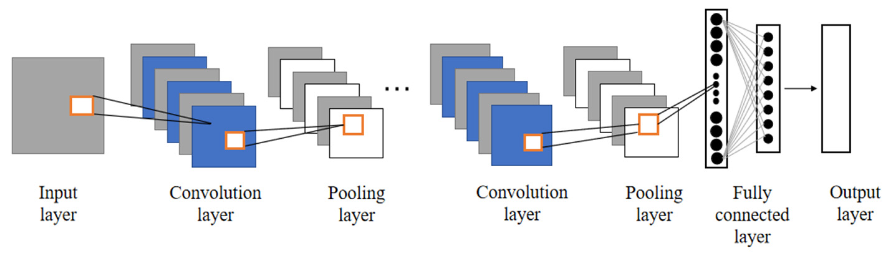
2.1. Convolutional Neural Network

A convolutional neural network (CNN) [41] is a core algorithm, remarkable for its unique convolutional operation and multi-level structural features. The CNN comprises the input, convolutional, pooling, activation, fully connected, and output layers.
In the CNN architectures, the convolutional and pooling layers usually collaborate to achieve hierarchical feature extraction and dimensionality reduction. The fully connected layer acts as a further high-dimensional integration and abstraction of the down-scaled features obtained after the convolution and pooling process, and this layer learns to distill the key patterns in the information of these features and ultimately outputs the prediction results for classification or regression. The CNN’s overall structure is shown in Figure 1.
(1) Convolution Layer
The convolutional layer extends and efficiently represents the essential characteristics of the input data, which performs feature extraction operations on each local region by applying a convolutional kernel to slide over the input data or previous feature maps. By scanning the input data point-by-point, the convolution kernel traverses all potential locations as a means of extracting spatial properties. The convolutional layer’s formula is as follows:
y l ( i , j ) = K i l x l r j = j V 1 k i l j x l j + j
where k i l ( j ) denotes the ith convolution kernel’s j th weight coefficient of in the lth layer, x l r j is the region of the jth localized feature in the convolution operation of the lth layer, and V represents the width.
(2) Pooling Layer
The pooling layer reduces the dimension of the convolution result of the previous layer by implementing various pooling techniques, to reduce the dimension of the feature graph. This process helps to mitigate data complexity while retaining the key information. The maximum pooling technique is adopted in this study, which is used to update the feature map by extracting the maximum value in a set pooling window, and the maximum pooling formula is:
p l ( i , j ) = max j 1 W + 1 t jW a l ( i , t )
where a l i , j indicates the activation value output by the tth neuron of the ith feature map in layer l, p l i , j refers to the amount of features output by the tth neuron of the ith feature map in layer l after pooling and W denotes the size of the window.
(3) Activation Layer
The activation layer plays a key role in a convolutional neural network in converting linear operations into nonlinear operations. By introducing the activation function, the activation layer can effectively constrain the output of neurons within a predetermined interval and then transfer the regulated signals to the subsequent layers of the network to realize the orderly transmission and processing of information. For this study, ReLU is chosen as the neuron activity mechanism, and its expression is:
a l i , j = f y l i , j = m a x 0 , y l i , j
where a l i , j represents the activation state of a particular layer in the neural network and y l i , j represents the output.
(4) Fully Connected Layer
It is the fully connected layer that converts 2D characteristic graphs from the upper layer into 1D corresponding function vectors to implement feature integration. This process is realized through weight matrices and bias terms, and finally, the processed information is presented in a specific form through the output layer.

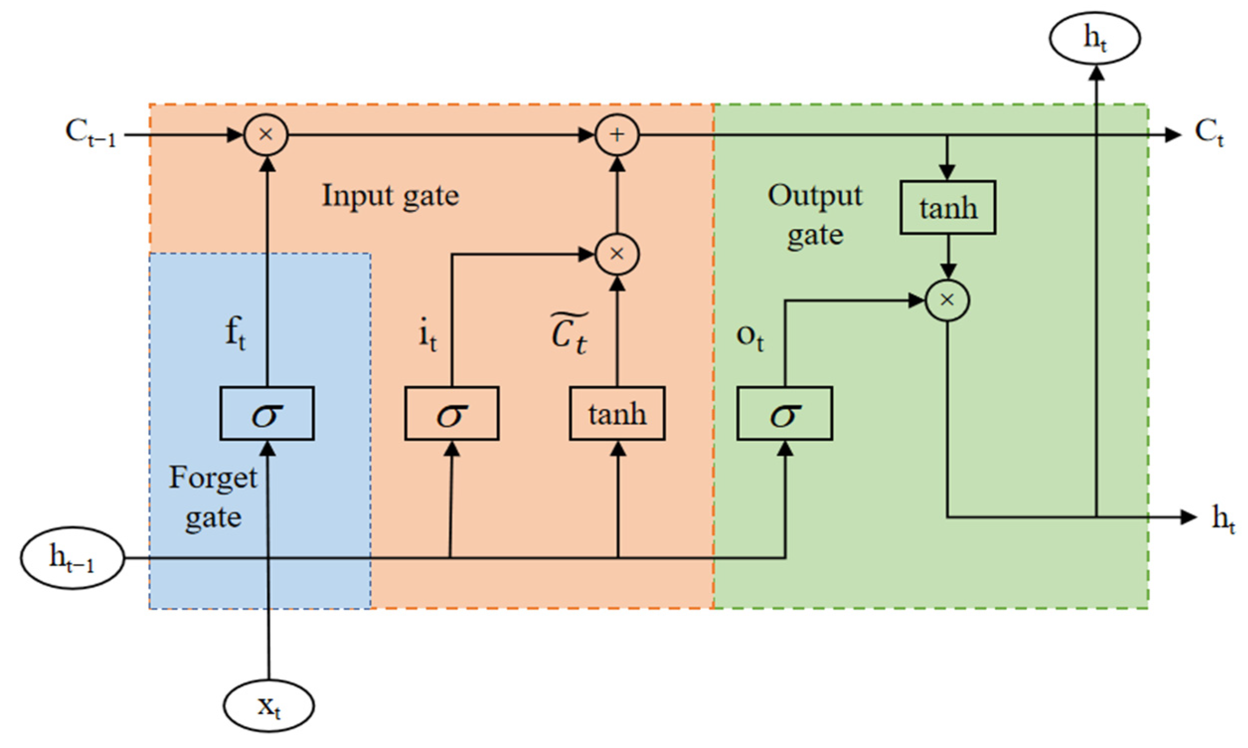
2.2. Long Short-Term Memory

Long short-term memory (LSTM) is an improved structure of recurrent neural networks which aims to improve the efficiency of processing time series data [42]. Using its particular gating algorithm, the LSTM successfully tackles the difficulties of vanishing and bursting gradients. Specifically, the LSTM includes the three key components of input, forgetting, and output gate. Working in tandem, these gates regulate the inflow, maintenance, and outflow of information, ensuring efficient transmission and memory retention of long sequences of information. The LSTM’s overall structure is shown in Figure 2.
(1) Input Gate i t
(2) The input gate filters messages, and is responsible for controlling the inflow or non-inflow of information and filtering out key information that can enter the neural network for subsequent processing. The input gate i t at time t in the LSTM’s expression is:
i t = S i g m o i d W i h t 1 , x t + b i
where x t denotes the input signal at time t and h t 1 denotes the output signal at the corresponding time. The weight matrix W i and the bias vector b i correspond to the relevant parameters, respectively.
(3) Forget Gate f t
As the core building block of LSTM, the forget gate assumes the important function of accurate screening and dynamic updating of cell state. The forget gate coefficients are decision parameters with values between 0 and 1 that determine whether the information in the cell state should be maintained or eliminated. This mechanism allows the LSTM network to maintain sensitivity and persistent memory for critical information when processing sequential data, thus significantly optimizing the performance and computational efficiency of the model. In the LSTM, the cell state at a specific moment t is denoted as C t ~ , the forget gate is denoted as f t , and the storage cell state is denoted as C t whose specific expression is shown below:
C t ~ = T a n h W c h t 1 , x t + b c
f t = S i g m o i d W f h t 1 , x t + b f
C t = f t C t 1 + i t C t ~
where C t ~ represents the weight matrix of the cell state, b c denotes the bias vector of the cell state, W f refers to the weight matrix of the oblivion gate, b f denotes the bias vector of the oblivion gate and C t 1 refers to the storage cell state at the previous moment.
(4) Output Gate o t
The output gate is responsible for calculating and determining the state that the unit should output, which depends on the input signal x t at the present moment, and the hidden layer output h t 1 at the preceding moment. The output gate o t at time t in the LSTM, and the expression of the final output state at time t is as follows:
o t = S i g m o i d W o h t 1 , x t + b o
h t = o t T a n h C t
where W o represents the weight matrix of the output gate and b o refers to the bias vector of the output gate.

2.3. Fruit Fly Optimization Algorithm

The fruit flies locate a food source through their sense of smell, and the algorithm uses the concentration of an odor as a navigation signal to guide the fruit fly toward the food source [43]. In this algorithmic mechanism, the concentration of odor perceived by a fruit fly shows a positive relationship with the spacing between it and the food source. During each iteration of the algorithm, the system tends to pick out those fruit flies that have the strongest perception of odor (the closest possible location to the food source) and carry out a localized, random search centered on its current location, a move that is intended to mimic the behavioral patterns of fruit flies searching for food in their natural environment. The detailed flow schematic of the fruit fly optimization algorithm (FOA) is presented in Figure 3.
Figure 3 succinctly illustrates the basic search mechanism of the fruit fly optimization algorithm (FOA). FOA imitates the foraging behavior of fruit flies, which have excellent olfactory and visual abilities. The following is a decomposition explanation of the diagram: (1) FOA: This represents the entire algorithm and its iterative process of finding the optimal solution. The coordinate axis represents the search space, with each point corresponding to a potential solution. (2) Center circle: This represents the best position (solution) currently found by the “fruit fly swarm”. Fruit flies initially scatter randomly around this location. (3) Flies: Fly1 (x1, y1) and Fly3 (x3, y3) both represent individual fruit flies in the fruit fly population. Each fruit fly explores the search space around its current optimal position. (4) Food: This represents the optimal or near-optimal solution that the algorithm is trying to find. (5) Dashed arrows: These represent the randomly dispersed paths of fruit flies from their current optimal position. They explore the surrounding area through small random movements. (6) Solid arrows: These represent the path taken by fruit flies towards the food source once its location is estimated. Fruit flies use their sense of smell to estimate the distance and direction of food sources. In algorithms, this is similar to evaluating the “odor” or “fitness” of the solution represented by the new position of fruit flies.
Among them, the FOA identifies the individual with the highest concentration based on different distributions of odor intensities and then uses an iterative strategy to dynamically update the spatial coordinates of the fruit fly population; hence, the problem is continually approached to the optimal solution. The FOA is shown as follows:
D i = X i 2 + Y i 2
S i = 1 D i
X i = X a x i s + R a n d ( F R )
Y i = Y a x i s + R a n d ( F R )
[ b e s t S m e l l , b e s t I n d e x ] = m i n S m e l l
S m e l l b e s t = b e s t S m e l l
X a x i s , Y a x i s = [ X b e s t I n d e x , Y b e s t I n d e x ]
where D i is the spatial distance from the fruit fly to the origin, X i , Y i is the direction of the fly, S i is the determination value of odor concentration, F R is for fruit fly out of range, X a x i s , Y a x i s is the population location, b e s t S m e l l is the most odor concentration value, X b e s t I n d e x , Y b e s t I n d e x is the location.

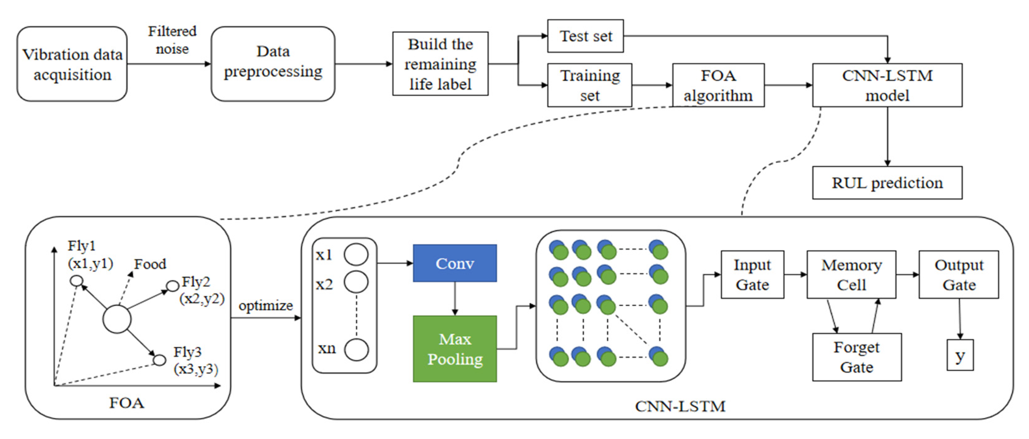
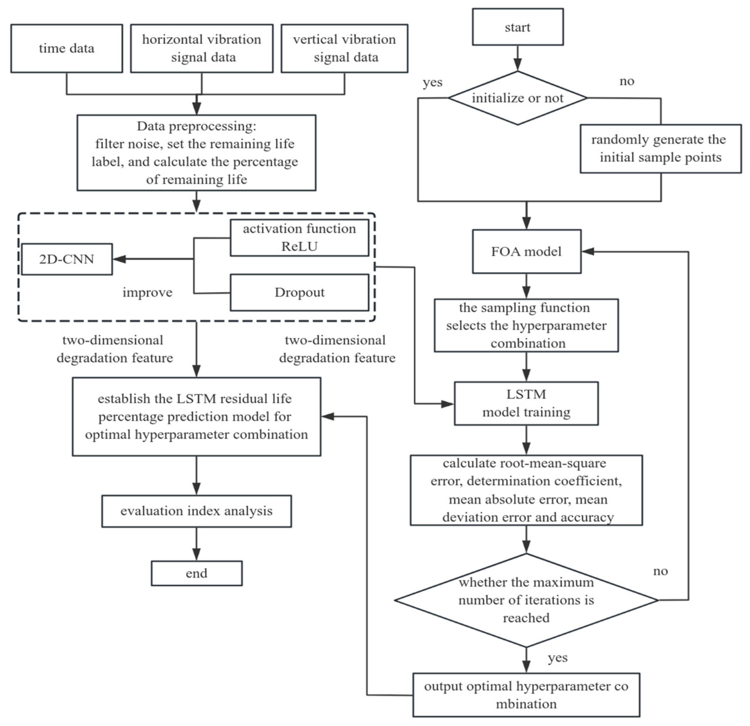
3. Proposed Methodology

This research aims to deeply analyze and upgrade precision in predicting rolling bearing RUL. To achieve this goal, an innovative prediction algorithm is designed and implemented, which skillfully combines the characteristics of the CNN and the LSTM, leveraging the specialties of both parties in signature abstraction and time-series analysis to complement each other. CNN extracts features from the visual representation of bearing vibration signals. These features do not directly correspond to specific physical damage but reflect the changes in vibration signals caused by the damage. As the bearing wears out, the energy of specific frequency components gradually increases, or frequency shifts occur. LSTM focuses on time series data, which can capture the dynamic characteristics of the bearing degradation process and use these time series data to identify the accumulation and development process of damage. On this basis, the prediction precision is effectively enhanced through fine-tuning the model performance by applying the FOA. By simulating the foraging process of fruit flies, it is possible to effectively search for the optimal combination of features in a high-dimensional feature space, improve the efficiency of CNN in the feature extraction stage, enhance the model’s attention to important features, reduce the interference of redundant information, and dynamically adjust the model’s hidden layer and threshold, optimize the hyperparameters of LSTM to adapt to different features of data, so that the model can respond more flexibly to changes in data when processing complex time series data, and improve prediction accuracy. Traditional optimization algorithms are often prone to fall into locally optimal solutions, while the FOA can effectively avoid this problem through its unique global search mechanism, helping the model to find more optimal solutions, thus improving the overall prediction performance, accelerating the convergence process of the model, significantly reducing the training time, and at the same time, maintaining or improving the prediction accuracy of the model. Shown in Figure 4 is the prediction flowchart of the model of this study, while Figure 5 further refines each specific prediction step of this process.
FOA-CNN-LSTM consists of three different models and has a certain level of complexity. The time complexity of CNN can be expressed as O k w h f , where k is the number of convolutional kernels in CNN, W is the width of the feature map, h is the height of the feature map, and f is the size of the convolutional kernels. The time complexity of LSTM can be expressed as O t h h + i + o , where t is the time step of LSTM, h is the number of hidden units, i is the number of input units and o is the number of output units. The time complexity of the FOA optimization process is affected by population size, maximum iteration times, and objective function evaluation times. Because the objective function evaluation of this method involves the forward propagation of CNN-LSTM, the time complexity of the FOA is related to the complexity of CNN-LSTM. Therefore, the total time complexity of the FOA-CNN-LSTM model can be approximated as O n m a x t k w h f + t h h + i + o , where n is the population size of FOA, and m a x t is the maximum number of iterations.

4. Test Verification

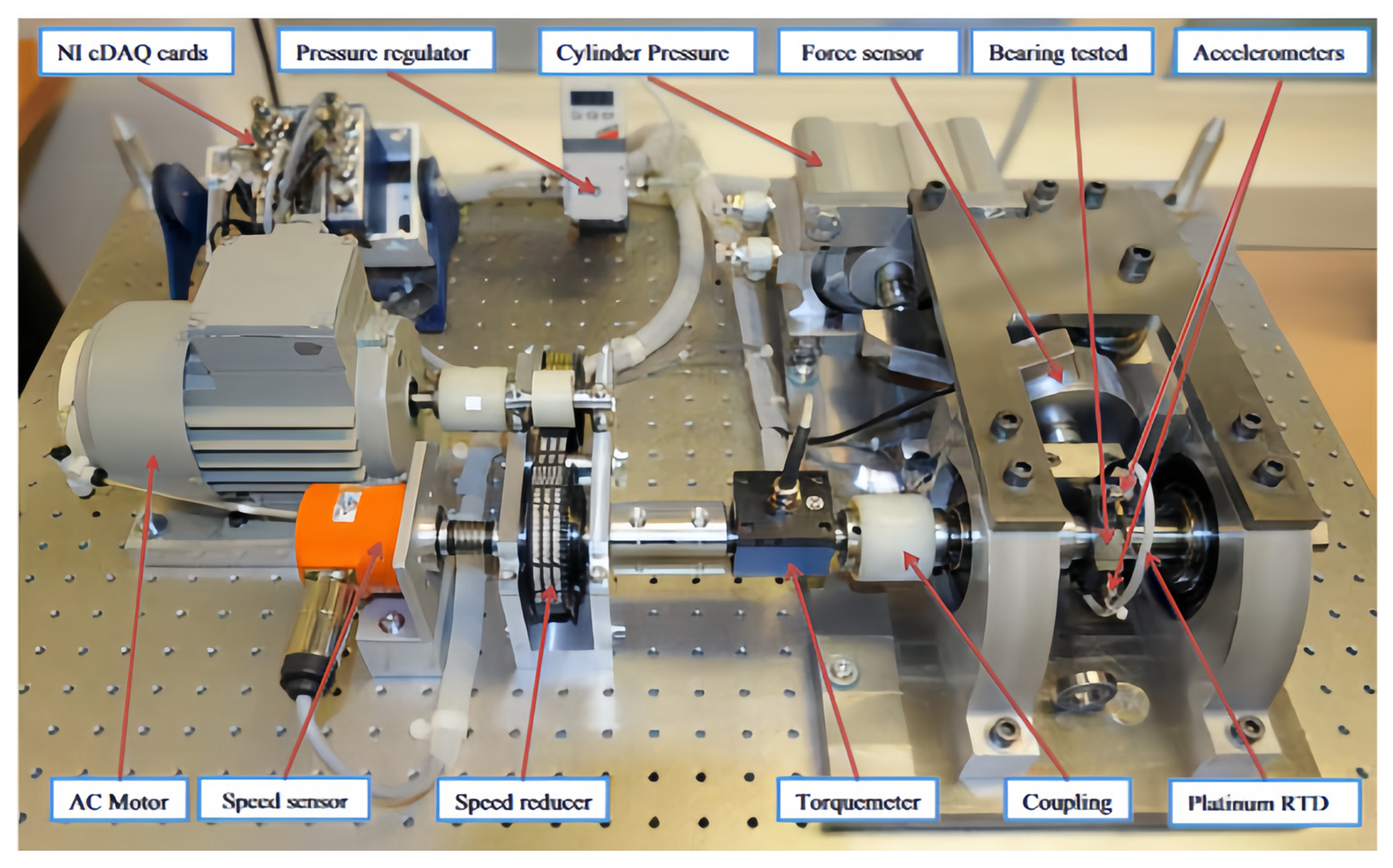
4.1. Data Description

To verify the practical application value and accuracy of the proposed method, the publicly available bearing dataset of the IEEE PHM 2012 challenge is selected for empirical analysis in this research to check the effect. This dataset recorded the degradation information of rolling bearings throughout their operating cycles. The experiments were conducted on a PRONOSTIA platform equipped with sensors for data acquisition. Each sensor was in charge of collecting information from the horizontal and vertical direction of vibration acceleration, the purpose was to monitor the operating condition of the bearing in real-time. During the data acquisition phase, the sensors sampled at 25.6 kHz with 2560 digital points every 0.1 s. Meanwhile, the system automatically recorded the timestamp of each data point, accurate to the hour, minute, second, and microsecond, and synchronously captured the corresponding horizontal and vertical vibration signals, which cycled through the process in 10 s intervals [44,45]. The PRONOSTIA table is displayed in Figure 6.
The dataset in the IEEE PHM 2012 challenge covered three different operating conditions that were designed to simulate a variety of operating scenarios that bearings may face in real-world applications. Specifically, the three different operating environments are set out in Table 1. This research seeks to demonstrate its validity and reliability by specifically selecting rolling bearing vibration data collected in operating conditions 1, 2, and 3, which are thoroughly tested and analyzed in depth.
As demonstrated in Figure 7, Figure 8 and Figure 9, the temporal waveforms of the vibration signals of rolling bearings 1-1, 2-1, and 3-2 in the horizontal and vertical directions have been meticulously recorded. The distribution characteristics of the bearing signals can also be found to show a gradual spreading trend as time progresses, even though there is an unavoidable noise component in the vibration signal. This trend suggests that the signal contains important characteristic information reflecting the gradual decay of the bearing health state.

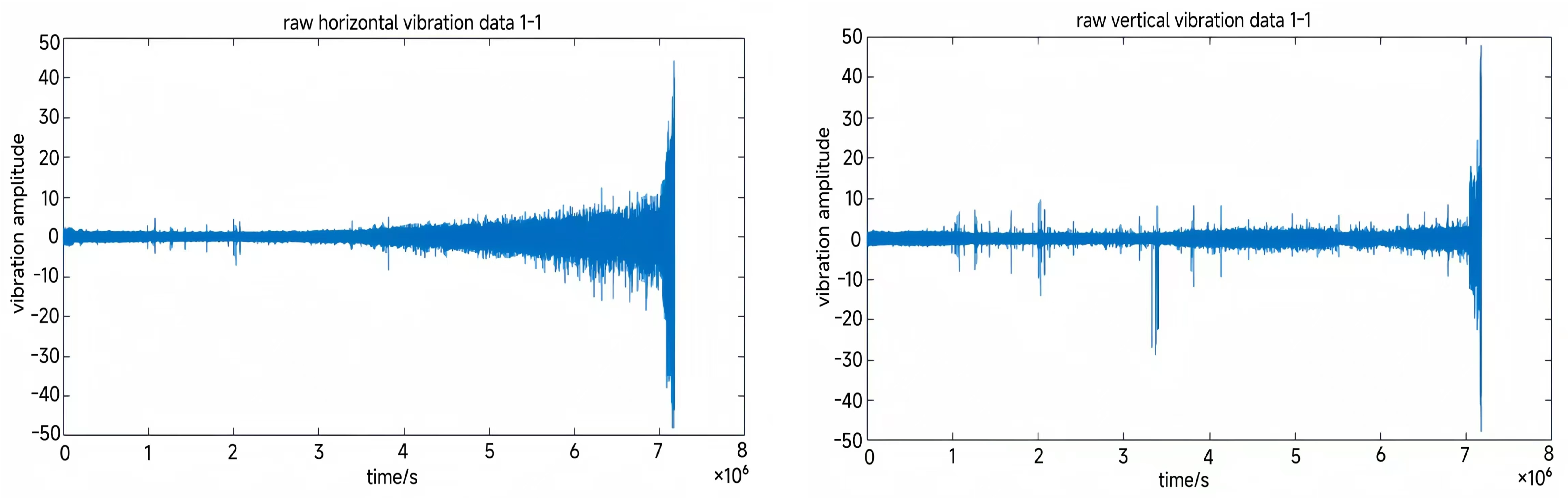
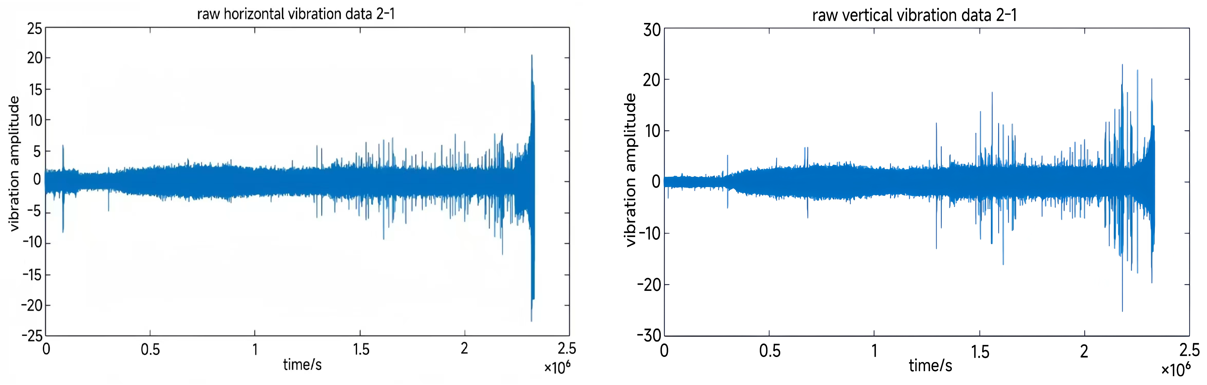
4.1.1. Data Pre-Processing

To diminish the effects of noise in the signal and the interference of variation between feature scales on prediction accuracy, a series of pre-processing preparations are implemented that delicately adjust both the horizontal and vertical vibration signal data. These pre-processing operations include outlier rejection, effective filtering of noise, and data normalization. The images after removing outliers and filtering noise are shown in Figure 10, Figure 11 and Figure 12.
In this paper, to improve the comparability of rolling bearing vibration signal data, the min–max normalization method is used for processing. This step effectively eliminates possible scale differences in the raw data and provides a more accurate input for subsequent data analysis and prediction. The min–max normalization method formula is as follows:
x n e w = x x m i n x m a x x m i n
where x is the rolling bearing’s first vibration signal, x m i n represents the minimum value in the signal, and x m a x is the maximum value in the signal. The minimum–maximum normalized vibration signal is denoted by x n e w .

4.1.2. Remaining Life Label Setting

After successfully acquiring the rolling bearing primary vibration data, it is then divided into training and testing sets using random assignment. However, given that remaining life labels are not directly available in the original dataset, closely related and accurate degradation labels must be constructed for the vibration data.
The percentage of real residual life E r i is employed that reflects the life labeling of the rolling bearing’s performance degradation condition. These labels are set to range from 0 to 1, where label 1 corresponds to the full health of the bearing, while label 0 represents that the bearing has completely failed. The formula for calculating the residual life percentage is described below:
E r i = A c t R U L i R U L i A c t R U L i × 100 %
where A c t R U L i represents the total life cycle of the rolling bearing during the test phase and R U L i denotes the actual operating time of the bearing.

4.2. Evaluation Metrics
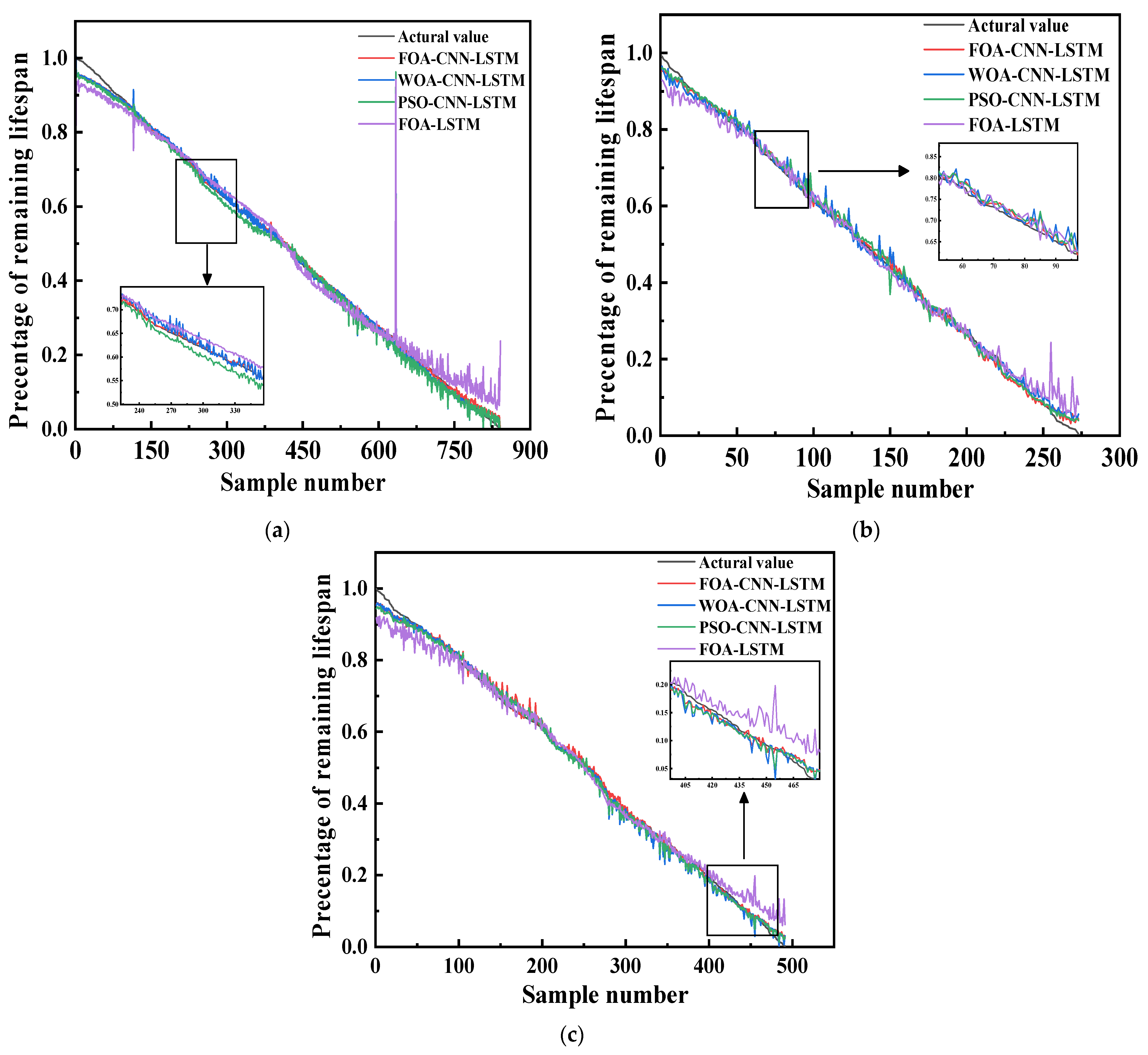
The RMSE (root mean square error), R2 (coefficient of determination), MAE (mean absolute error), and the accuracy between the forecast and the actual values of life remaining are selected as the core evaluation indexes so that the proposed rolling bearing life prediction method can be explored exhaustively and evaluated accurately. When evaluating the performance of the prediction algorithm, the reduction of RMSE and MAE values reflects the reduction of the deviation between the predicted value and the actual value, thus reflecting the improvement of the prediction accuracy. Similarly, both R2 and accuracy improvements indicate an increased consistency between the prediction results and the real data. The RMSE, R2, MAE, and accuracy calculations are detailed below:
R M S E = 1 n ( R U L A C T R U L ) 2
R 2 = 1 R U L A C T R U L 2 / ( A C T R U L A C T R U L ¯ ) 2
M A E = 1 n | R U L A C T R U L |
A c c u r a c y = 1 M A E A C T R U L ¯ 100 %
where n denotes the overall sample count, R U L refers to the predicted values, A C T R U L indicates the actual observed values and A C T R U L ¯ is the average of all true values.

4.3. Test Results

In this paper, the PHM 2012 rolling bearing dataset under conditions 1, 2, and 3 are exhaustively tested and analyzed. In each condition, the training data are delineated at 70%, and the remaining 30% are used as validation data to construct several sub-datasets.
After careful parameter tuning and model optimization, this study finally establishes a network architecture whose core components include two 2D convolutional layers designed to accurately capture the spatial features of the data, a pooling layer that effectively reduces the data dimensions while retaining the core information, two LSTM layers that are introduced to capture complex temporal dependencies and a fully connected layer that integrates features extracted in all of the previous phases and maps them to the final prediction. When constructing the model, the ReLU (rectified linear unit) is the preferred function for activation. This choice significantly enhances the model’s representation of nonlinear features, which in turn strengthens its ability to uncover potentially complex patterns. To prevent overfitting of the model, this study introduces a dropout layer with a ratio of 0.1 in the training phase. By randomly ignoring some of the neuron connections, this method significantly improves the generalization ability of the model, enabling it to maintain stable performance on unseen data. Meanwhile, to optimize the parameters in the hidden layer of the CNN-LSTM model, this study uses the FOA for several experiments. In the experiment, the number of fruit fly species is fixed at 10, the maximum number of iterations is 5, and the upper and lower limits of the weight threshold are 0 and 1, respectively.
Let us take bearing 1-1 as an example by carefully examining the data results shown in Figure 13. It can be seen that the proposed method exhibits excellent fitting results on both the training and testing sets. It effectively retrieves and captures key feature information of bearing performance degradation from training samples and performs well in predicting the remaining life of bearings, almost accurately predicting the percentage of remaining life at any point in the bearing life.

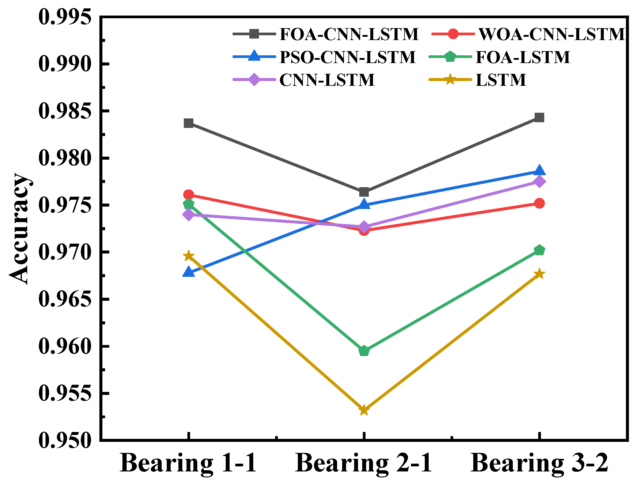
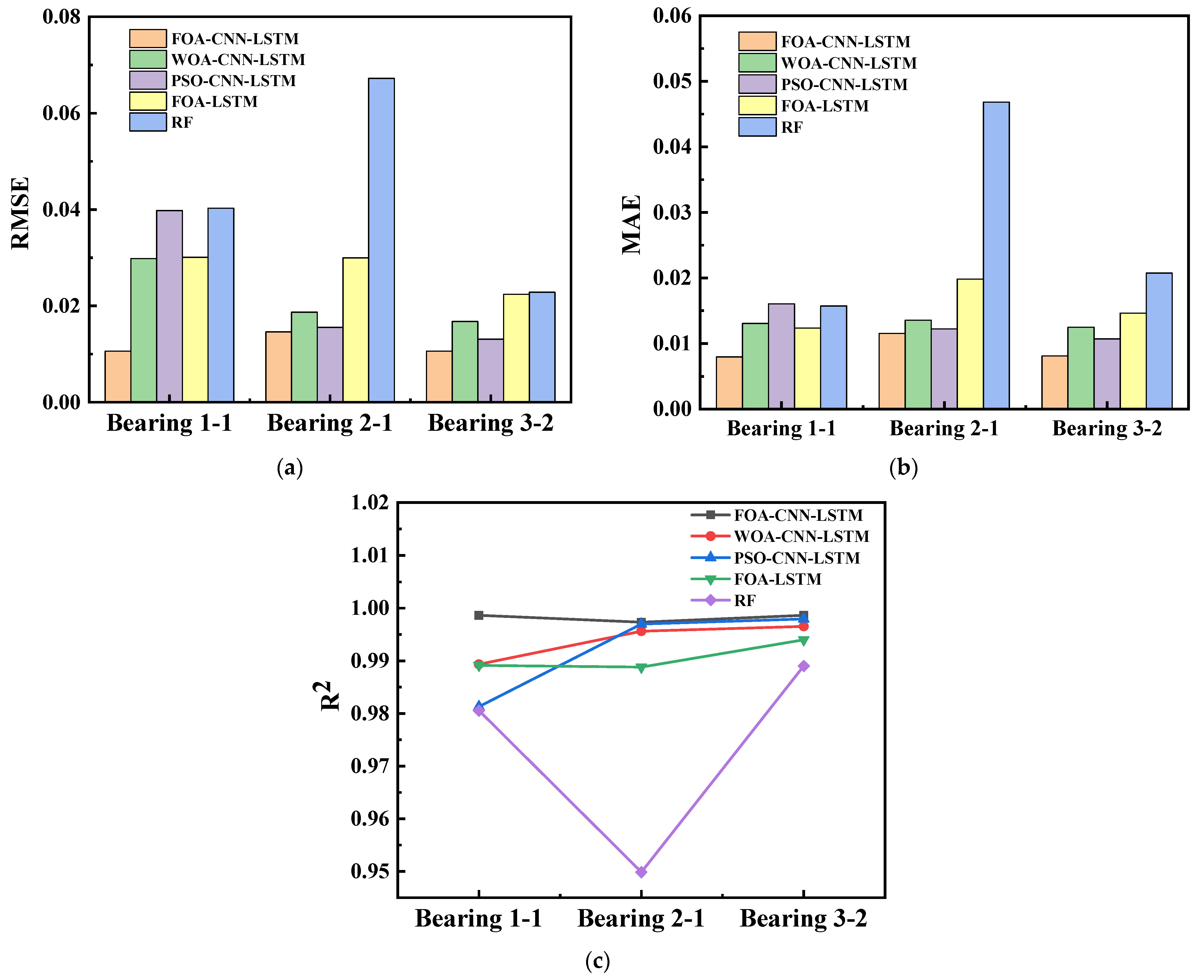
4.4. Contrast Experiments and Comparative Analysis

This article randomly divides the time feature vectors, horizontal vibration signal feature vectors, and vertical vibration signal feature vectors of bearings 1-1, 2-1, and 3-2 into training and testing sets in a 7:3 ratio. The effectiveness of this model in predicting the RUL of rolling bearings has been confirmed through multiple comparative experiments. In these experiments, this paper’s method is compared and analyzed in depth with the WOA-CNN-LSTM, RF, PSO-CNN-LSTM, FOA-LSTM, LSTM, and CNN-LSTM networks. The network parameters of all the comparison methods are set uniformly in the comparison experiments to make them consistent with the forecast methods proposed in this study and to ensure that the experimental results can accurately reflect the different performances among different methods.
In this paper, the performance of different RUL prediction methods is comprehensively evaluated using RMSE, R2, and accuracy as evaluation metrics. Table 2 and Table 3 show the accuracy, RMSE, R2, and MAE of the training data for different models. Table 4 and Table 5 show the accuracy, RMSE, R2, and MAE of the testing data for different models.
The method in this paper adds the FOA optimization algorithm after selecting CNN for extracting features and LSTM for mining time series. As can be seen from Figure 14, adding an optimization algorithm has higher prediction accuracy than no optimization algorithm, and the optimization algorithm chosen in this paper has better results.
To investigate the effectiveness of the FOA-CNN-LSTM, we designed an ablation study for the proposed method by comparing the FOA-CNN-LSTM with the WOA-CNN-LSTM, PSO-CNN-LSTM, and the FOA-LSTM in the experiments. From Figure 15, it can be seen that the predicted values of this paper’s method on the bearing 1-1, 2-1, and 3-2 testing sets are closer to the true value curves, which shows that the optimization algorithm used in this paper is better than other optimization algorithms.
To illustrate the advantages of the FOA-CNN-LSTM, the popular algorithm RF is included for comparison with other optimization algorithms. As can be seen from Figure 16, the RMSE and MAE values of this method are lower than other prediction methods, and R2 is higher than other methods. It can be seen that the method proposed in this paper is superior compared to adding other optimization algorithms or other popular algorithms.

5. Conclusions

This research proposes a novel rolling-bearing RUL forecasting algorithm called FOA-CNN-LSTM. This model successfully combines the core strengths of CNN and LSTM to provide an in-depth analysis for data feature capture. CNN has excellent capabilities in spatial feature extraction and is able to automatically identify and extract local features in the data so as to effectively process high-dimensional data such as images and videos. On the other hand, the LSTM is good at capturing long-term dependencies in time series and can deal with dynamic changes and contextual information in sequential data. By combining the advantages of these two networks, the CNN-LSTM model is not only able to deeply analyze the spatial features of the data but also effectively understand its dynamic characteristics over time. Meanwhile, through the application of the FOA algorithm, successive optimizations of the internal parameters and their thresholds of the CNN-LSTM model are enforced, of which the model is directed to explore the global optimal resolution. With this optimization, the prediction accuracy and confidence of the bearing RUL are significantly improved. Subsequently, the robustness of the FOA-CNN-LSTM model is verified using three sets of rolling bearing datasets. Through the careful analysis of the prediction effect graphs, the FOA-CNN-LSTM model proposed in this paper demonstrates significant advantages in comparison with other comparative models, including WOA-CNN-LSTM, RF, PSO-CNN-LSTM, FOA-LSTM, CNN-LSTM, and LSTM. Specifically, the FOA-CNN-LSTM model generates the highest degree of agreement between predicted and actual values, indicating that the model is more capable of capturing data features and dynamic changes. The evaluation metrics show that the prediction method in this paper has the smallest RMSE and MAE, the closest R2 to 1, and the highest accuracy compared to other algorithms. In the task of predicting RUL, the model constructed in this study exhibits the highest prediction accuracy.

Author Contributions

Conceptualization, J.S. and Z.J.; data curation, M.J. and Q.W.; formal analysis, Z.J.; funding acquisition, H.Z.; methodology, J.S. and M.J.; software, J.S.; supervision, H.Z.; validation, J.S., H.Z., Y.M. and Z.H.; visualization, H.Z.; writing—original draft, J.S.; writing—review and editing, J.S., H.Z. and Q.W. All authors have read and agreed to the published version of the manuscript.

Funding

This research was funded by the State Administration for Market Regulation Science and Technology Plan Project under Grant No.2023MK228, National Key Research and Development Plan Young Scientists Project under Grant No.2021YFF0603400, Core Project of The “Eagle Plan” of the Zhejiang Provincial Market Supervision and Administration Bureau under Grant No.CY2022220, Zhejiang Provincial Natural Science Foundation of China under Grant No.LQ21E050019.

Data Availability Statement

The data presented in this study are available request from the corresponding author.

Conflicts of Interest

The authors declare no conflicts of interest.

Abbreviations

The following abbreviations are used in this manuscript:
RULRemaining Useful Life
CNNConvolutional Neural Network
LSTMLong Short-Term Memory Network
FOAFruit Fly Optimization Algorithm
WOAWhale Optimization Algorithm
PSOParticle Swarm Optimization
RFRandom Forest
RMSERoot mean square error
MAEMean absolute error
R2Coefficient of determination
EriThe percentage of real residual life

References

  1. Babu, T.N.; Saraya, J.; Singh, K.; Prabha, D.R. Rolling element bearing fault diagnosis using discrete mayer wavelet and fault classification using machine learning algorithms. J. Vib. Eng. Technol. 2025, 13, 87. [Google Scholar] [CrossRef]
  2. Mao, W.T.; Liu, Y.M.; Ding, L.; Safian, A.; Liang, X.H. A new structured domain adversarial neural network for transfer fault diagnosis of rolling bearings under different working conditions. IEEE Trans. Instrum. Meas. 2021, 70, 3509013. [Google Scholar] [CrossRef]
  3. Ma, S.J.; Zhang, X.H.; Yan, K.; Zhu, Y.S.; Hong, J. A study on bearing dynamic features under the condition of multiball-cage collision. Lubricants 2022, 10, 9. [Google Scholar] [CrossRef]
  4. Cheng, H.; Kong, X.G.; Chen, G.; Wang, Q.B.; Wang, R.B. Transferable convolutional neural network based remaining useful life prediction of bearing under multiple failure behaviors. Measurement 2021, 168, 108286. [Google Scholar] [CrossRef]
  5. Xu, J.; Duan, S.Y.; Chen, W.W.; Wang, D.F.; Fan, Y.Q. SACGNet: A remaining useful life prediction of bearing with self-attention augmented convolution GRU network. Lubricants 2022, 10, 21. [Google Scholar] [CrossRef]
  6. Ansean, D.; Dubarry, M.; Devie, A.; Liaw, B.Y.; Garcia, V.M.; Viera, J.C.; Gonzalez, M. Fast charging technique for high power LiFePO4 batteries: A mechanistic analysis of aging. J. Power Sources 2016, 321, 201–209. [Google Scholar] [CrossRef]
  7. Londhe, N.D.; Arakere, N.K.; Haftka, R.T. Reevaluation of rolling element bearing load-Life equation based on fatigue endurance data. Tribol. Trans. 2015, 58, 815–828. [Google Scholar] [CrossRef]
  8. Londhe, N.D.; Arakere, N.K.; Subhash, G. Extended hertz theory of contact mechanics for case-hardened steels with implications for bearing fatigue life. J. Tribol. 2018, 140, 021401. [Google Scholar] [CrossRef]
  9. Mao, W.T.; He, J.L.; Zuo, M.J. Predicting remaining useful life of rolling bearings based on deep feature representation and transfer learning. IEEE Trans. Instrum. Meas. 2020, 69, 1594–1608. [Google Scholar] [CrossRef]
  10. Xie, G.; Peng, X.; Li, X.; Hei, X.H.; Hu, S.L. Remaining useful life prediction of lithium-ion battery based on an improved particle filter algorithm. Can. J. Chem. Eng. 2020, 98, 1365–1376. [Google Scholar] [CrossRef]
  11. Wang, Y.Z.; Ni, Y.L.; Li, N.; Lu, S.; Zhang, S.D.; Feng, Z.B.; Wang, J.G. A method based on improved ant lion optimization and support vector regression for remaining useful life estimation of lithium-ion batteries. Energy Sci. Eng. 2019, 7, 2797–2813. [Google Scholar] [CrossRef]
  12. Ma, G.J.; Zhang, Y.; Cheng, C.; Zhou, B.T.; Hu, P.C.; Yuan, Y. Remaining useful life prediction of lithium-ion batteries based on false nearest neighbors and a hybrid neural network. Appl. Energy 2019, 253, 113626. [Google Scholar] [CrossRef]
  13. Ma, P.; Li, G.F.; Zhang, H.L.; Wang, C.; Li, X.K. Prediction of remaining useful life of rolling bearings based on multiscale efficient channel attention CNN and bidirectional GRU. IEEE Trans. Instrum. Meas. 2024, 73, 2508413. [Google Scholar] [CrossRef]
  14. Han, G.D.; Cao, Y.P.; Xu, Z.Q.; Wang, W.Y. Research on the SMIV-1DCNN remaining useful life prediction method for marine gas turbine. J. Eng. Therm. Energy Power 2022, 37, 25–32. [Google Scholar] [CrossRef]
  15. Li, X.; Zhang, W.; Ding, Q. Deep learning-based remaining useful life estimation of bearings using multi-scale feature extraction. Reliab. Eng. Syst. Saf. 2019, 182, 208–218. [Google Scholar] [CrossRef]
  16. Wang, X.; Mao, D.X.; Li, X.D. Bearing fault diagnosis based on vibro-acoustic data fusion and 1D-CNN network. Measurement 2021, 173, 108518. [Google Scholar] [CrossRef]
  17. Liu, Y.; Dan, B.B.; Yi, C.C.; Li, S.H.; Yan, X.G.; Xiao, H. Similarity indicator and CG-CGAN prediction model for remaining useful life of rolling bearings. Meas. Sci. Technol. 2024, 35, 086107. [Google Scholar] [CrossRef]
  18. Yan, X.; Jin, X.P.; Jiang, D.; Xiang, L. Remaining useful life prediction of rolling bearings based on CNN-GRU-MSA with multi-channel feature fusion. Nondestruct. Test. Eval. 2024, 1–26. [Google Scholar] [CrossRef]
  19. Deng, L.F.; Li, W.; Yan, X.H. An intelligent hybrid deep learning model for rolling bearing remaining useful life prediction. Nondestruct. Test. Eval. 2024, 1–28. [Google Scholar] [CrossRef]
  20. Wang, Z.Y.; Guo, J.Y.; Wang, J.; Yang, Y.L.; Dai, L.; Huang, C.G.; Wan, J.L. A deep learning based health indicator construction and fault prognosis with uncertainty quantification for rolling bearings. Meas. Sci. Technol. 2023, 34, 105105. [Google Scholar] [CrossRef]
  21. He, J.L.; Wu, C.C.; Luo, W.; Qian, C.H.; Liu, S.Y. Remaining useful life prediction and uncertainty quantification for bearings based on cascaded multiscale convolutional neural network. IEEE Trans. Instrum. Meas. 2024, 73, 3506713. [Google Scholar] [CrossRef]
  22. Yang, B.Y.; Liu, R.N.; Zio, E. Remaining useful life prediction based on a double-convolutional neural network architecture. IEEE Trans. Ind. Electron. 2019, 66, 9521–9530. [Google Scholar] [CrossRef]
  23. Wu, C.B.; You, A.G.; Ge, M.F.; Liu, J.; Zhang, J.C.; Chen, Q. A novel multi-scale gated convolutional neural network based on informer for predicting the remaining useful life of rotating machinery. Meas. Sci. Technol. 2024, 35, 126138. [Google Scholar] [CrossRef]
  24. Liu, Z.H.; Meng, X.D.; Wei, H.L.; Chen, L.; Lu, B.L.; Wang, Z.H.; Chen, L. A regularized LSTM method for predicting remaining useful life of rolling bearings. Int. J. Autom. Comput. 2021, 18, 581–593. [Google Scholar] [CrossRef]
  25. Li, L.Y.; Wang, H.R.; Zhu, G.F. Remaining useful life prediction of turbofan engine based on improved 1D-CNN and LSTM. J. Eng. Therm. Energy Power 2023, 38, 194–202. [Google Scholar] [CrossRef]
  26. Marei, M.; Li, W.D. Cutting tool prognostics enabled by hybrid CNN-LSTM with transfer learning. Int. J. Adv. Manuf. Technol. 2022, 118, 817–836. [Google Scholar] [CrossRef]
  27. Lei, N.; Tang, Y.F.; Li, A.; Jiang, P.C. Research on the remaining life prediction method of rolling bearings based on optimized TPA-LSTM. Machines 2024, 12, 224. [Google Scholar] [CrossRef]
  28. Song, F.; Wang, Z.H.; Liu, X.Q.; Ren, G.A.; Liu, T. Remaining life prediction of rolling bearings with secondary feature selection and BSBiLSTM. Meas. Sci. Technol. 2024, 35, 076127. [Google Scholar] [CrossRef]
  29. Yao, X.J.; Zhu, J.J.; Jiang, Q.S.; Yao, Q.; Shen, Y.H.; Zhu, Q.X. RUL prediction method for rolling bearing using convolutional denoising autoencoder and bidirectional LSTM. Meas. Sci. Technol. 2024, 35, 035111. [Google Scholar] [CrossRef]
  30. Cai, S.; Zhang, J.W.; Li, C.; He, Z.Q.; Wang, Z.M. A rul prediction method of rolling bearings based on degradation detection and deep BiLSTM. Electron. Res. Arch. 2024, 32, 3145–3161. [Google Scholar] [CrossRef]
  31. Zhang, X.G.; Yang, J.Z.; Yang, X.M. Residual life prediction of rolling bearings based on a CEEMDAN algorithm fused with CNN-attention-based bidirectional LSTM modeling. Processes 2024, 12, 8. [Google Scholar] [CrossRef]
  32. Yang, L.; Jiang, Y.B.; Zeng, K.; Peng, T. Rolling bearing remaining useful life prediction based on CNN-VAE-MBiLSTM. Sensors 2024, 24, 2992. [Google Scholar] [CrossRef]
  33. Wei, L.P.; Peng, X.Y.; Cao, Y.P. Enhanced fault diagnosis of rolling bearings using an improved inception-lstm network. Nondestruct. Test. Eval. 2024, 1–20. [Google Scholar] [CrossRef]
  34. Sun, W.Q.; Wang, Y.; You, X.Y.; Zhang, D.; Zhang, J.Y.; Zhao, X.H. Optimization of variational mode decomposition-convolutional neural network-bidirectional long short term memory rolling bearing fault diagnosis model based on improved dung beetle optimizer algorithm. Lubricants 2024, 12, 239. [Google Scholar] [CrossRef]
  35. Yang, J.Z.; Zhang, X.G.; Liu, S.; Yang, X.M.; Li, S.F. Rolling bearing residual useful life prediction model based on the particle swarm optimization-optimized fusion of convolutional neural network and bidirectional long-short-term memory-multihead self-attention. Electronics 2024, 13, 2120. [Google Scholar] [CrossRef]
  36. Ni, Q.; Ji, J.C.; Feng, K. Data-Driven Prognostic Scheme for Bearings Based on a Novel Health Indicator and Gated Recurrent Unit Network. IEEE Trans. Industr. Inform. 2023, 19, 1301–1311. [Google Scholar] [CrossRef]
  37. Huang, K.; Jia, G.Z.; Jiao, Z.Y.; Luo, T.Y.; Wang, Q.; Cai, Y.J. MSTAN: Multi-scale spatiotemporal attention network with adaptive relationship mining for remaining useful life prediction in complex systems. Meas. Sci. Technol. 2024, 35, 125019. [Google Scholar] [CrossRef]
  38. Cui, L.L.; Xiao, Y.C.; Liu, D.D.; Han, H.G. Digital twin-driven graph domain adaptation neural network for remaining useful life prediction of rolling bearing. Reliab. Eng. Syst. Saf. 2024, 245, 109991. [Google Scholar] [CrossRef]
  39. Bienefeld, C.; Kirchner, E.; Vogt, A.; Kacmar, M. On the importance of temporal information for remaining useful life prediction of rolling bearings using a random forest regressor. Lubricants 2022, 10, 67. [Google Scholar] [CrossRef]
  40. Lu, X.C.; Yao, X.J.; Jiang, Q.S.; Shen, Y.H.; Xu, F.Y.; Zhu, Q.X. Remaining useful life prediction model of cross-domain rolling bearing via dynamic hybrid domain adaptation and attention contrastive learning. Comput. Ind. 2024, 164, 104172. [Google Scholar] [CrossRef]
  41. Li, C.; Chen, H.X.; Han, Y.; Zuo, S.J.; Zhao, L.G. A survey of convolution neural networks in deep learning algorithm. J. Electron. Test. 2018, 23, 61–62. [Google Scholar] [CrossRef]
  42. Yu, Y.; Si, X.S.; Hu, C.H.; Zhang, J.X. A review of recurrent neural networks: LSTM cells and network architectures. Neural Comput. 2019, 31, 1235–1270. [Google Scholar] [CrossRef]
  43. Wang, H.Y.; Song, W.Q.; Zio, E.; Kudreyko, A.; Zhang, Y.J. Remaining useful life prediction for lithium-ion batteries using fractional brownian motion and fruit-fly optimization algorithm. Measurement 2020, 161, 2069–2080. [Google Scholar] [CrossRef]
  44. Ren, L.; Sun, Y.Q.; Wang, H.; Zhang, L. Prediction of bearing remaining useful life with deep convolution neural network. IEEE Access 2018, 6, 13041–13049. [Google Scholar] [CrossRef]
  45. Nectoux, P.; Gouriveau, R.; Medjaher, K.; Ramasso, E.; Chebel-Morello, B.; Zerhouni, N.; Varnier, C. An experimental platform for bearings accelerated degradation tests. In Proceedings of the IEEE International Conference on Prognostics and Health Management, PHM’12, Denver, CO, USA, 18–21 June 2012; pp. 1–8. [Google Scholar]
Figure 1. CNN structure diagram.
Lubricants 13 00081 g001
Figure 2. LSTM schematic.
Lubricants 13 00081 g002
Figure 3. Schematic diagram of FOA process.
Lubricants 13 00081 g003
Figure 4. FOA-CNN-LSTM model bearing life prediction flowchart.
Lubricants 13 00081 g004
Figure 5. Rolling bearing life prediction process chart.
Lubricants 13 00081 g005
Figure 6. PRONOSTIA table.
Lubricants 13 00081 g006
Figure 7. Rolling bearing 1-1 vibration signal waveforms.
Lubricants 13 00081 g007
Figure 8. Rolling bearing 2-1 vibration signal waveforms.
Lubricants 13 00081 g008
Figure 9. Rolling bearing 3-2 vibration signal waveforms.
Lubricants 13 00081 g009
Figure 10. Rolling bearing 1-1 vibration signal waveforms after pre-processing.
Lubricants 13 00081 g010
Figure 11. Rolling bearing 2-1 vibration signal waveforms after pre-processing.
Lubricants 13 00081 g011
Figure 12. Rolling bearing 3-2 vibration signal waveforms after pre-processing.
Lubricants 13 00081 g012
Figure 13. The predicted and true values of the FOA-CNN-LSTM model on 1-1 bearings in the training and testing set.
Lubricants 13 00081 g013
Figure 14. Accuracy of the prediction methods on the testing data.
Lubricants 13 00081 g014
Figure 15. Comparative experimental results with different training methods (a) bearing 1-1, (b) bearing 2-1, (c) bearing 3-2.
Lubricants 13 00081 g015
Figure 16. RMSE, MAE and R2 of the prediction methods on the testing data (a) RMSE, (b) MAE, (c) R2.
Lubricants 13 00081 g016
Table 1. Operating conditions of rolling bearing data.
Operating ConditionRolling Bearing NumberLoad/NRotation Speed/(r·min−1)
Operating condition 11-1, 1-2, 1-3
1-4, 1-5, 1-6, 1-7
40001800
Operating condition 22-1, 2-2, 2-3
2-4, 2-5, 2-6, 2-7
42001650
Operating condition 33-1, 3-2, 3-350001500
Table 2. Accuracy and R2 of different prediction methods on the training set.
MethodsAccuracyR2
1-12-13-21-12-13-2
FOA-CNN-LSTM98.24%97.63%98.39%0.992280.997170.99876
WOA-CNN-LSTM97.61%97.28%97.56%0.993720.995330.99701
PSO-CNN-LSTM97.24%97.57%98.00%0.99650.997240.99817
FOA-LSTM97.62%95.87%97.21%0.993380.989610.99522
CNN-LSTM97.61%97.42%97.70%0.994010.996650.99734
LSTM97.41%95.34%96.21%0.990120.987890.99325
RF96.84%94.54%96.88%0.991090.980240.98901
Table 3. RMSE and MAE of different prediction methods on the training set.
MethodsRMSEMAE
1-12-13-21-12-13-2
FOA-CNN-LSTM0.0253050.0154860.0101590.00889530.011960.007936
WOA-CNN-LSTM0.0228580.0198840.0158510.0120850.0137090.012148
PSO-CNN-LSTM0.0170060.0152680.0123260.0138170.0122320.009977
FOA-LSTM0.0234760.0296450.0199480.0119340.0207930.01404
CNN-LSTM0.0221370.0168420.0149870.0118760.0129940.011439
LSTM0.0284830.0320030.0240210.012960.0235010.018265
RF0.0272490.0398690.0207420.0233380.0273620.015766
Table 4. Accuracy and R2 of different prediction methods on the testing set.
MethodsAccuracyR2
1-12-13-21-12-13-2
FOA-CNN-LSTM98.37%97.64%98.43%0.998660.997340.99865
WOA-CNN-LSTM97.32%97.23%97.52%0.989330.995640.99655
PSO-CNN-LSTM96.78%97.50%97.86%0.981310.996990.99796
FOA-LSTM97.51%95.95%97.02%0.989150.988810.99401
CNN-LSTM97.40%97.27%97.75%0.991080.996230.99737
LSTM96.96%95.32%96.77%0.988470.988230.99284
RF95.37%90.56%95.73%0.980550.949860.98901
Table 5. RMSE and MAE of different prediction methods on the testing set.
MethodsRMSEMAE
1-12-13-21-12-13-2
FOA-CNN-LSTM0.0105990.0145960.0106520.00794010.0115340.0080978
WOA-CNN-LSTM0.0298180.0187070.0167780.013060.0135620.012486
PSO-CNN-LSTM0.0397880.0155430.013070.0160420.0122190.010699
FOA-LSTM0.0300770.0299710.0223870.0123540.0198130.01463
CNN-LSTM0.0291870.01740.0145990.0132350.0133730.011311
LSTM0.0315820.0307290.0240210.0149930.0228980.017483
RF0.0402640.0672220.0228230.0233380.0468270.020742
Disclaimer/Publisher’s Note: The statements, opinions and data contained in all publications are solely those of the individual author(s) and contributor(s) and not of MDPI and/or the editor(s). MDPI and/or the editor(s) disclaim responsibility for any injury to people or property resulting from any ideas, methods, instructions or products referred to in the content.

