Abstract
Lubrication is a critical process in cold strip rolling, and the accurate characterization of lubrication characteristics is an essential factor affecting the strip quality. The roll bending and tilting roll in the flatness actuators change the loaded roll gap profile and affect the lubrication characteristics by flatness dynamic correction, thus the mismatch between the actual and setting values of the lubrication status factor. Firstly, the flatness deviation correction model of roll bending and tilting roll based on the key information of the rolling process is established according to the high-order flatness target. Secondly, the characterization of the instantaneous oil film thickness in the work zone based on the loaded roll gap profile is derived from Reynolds’ equation. Finally, the explicit characterization method of the lubrication status factor in the rolling force model of the final stand is established with the work roll bending, tilting roll, and instantaneous oil film thickness of the work zone as variables, relying on the UCM five-stand, six-roll tandem cold rolling mill. The statistical evaluation and application results show that the mentioned optimization method can improve the setting accuracy of the rolling force by about 60% and the after-rolling gauge accuracy by about 50%.
1. Introduction
Cold strip rolling products are an important part of the iron and steel industry [1]. Their quality and production have long been key indicators of a country’s overall strength [2]. Lubrication and friction are the core parts of the cold strip rolling and are key process aspects that determine the stability of the strip quality [3,4].
Based on hydrodynamic lubrication, an oil film is formed in the loaded roll gap due to the rolling speed and the lubricant viscosity characteristics, thus reducing the asperity contact area between the work rolls and the strip and achieving lubrication [5,6]. The oil film’s thickness and corresponding distribution characteristics in the loaded roll gap directly determine and influence the lubrication characteristics during the strip rolling process.
In the rolling procedure of the UCM six-roll, five-stand tandem cold rolling mill, the final stand, besides bearing part of the reduction to ensure the quality of the strip gauge, is more to adjust the flatness quality of the cold strip rolling [7]. There are four types of flatness actuators, including roll bending, intermediate roll transverse shifting (IRS), tilting rolls (TR), and segmented cooling [8]. The roll bending includes the intermediate roll bending (IRB) and the work roll bending (WRB), and the tilting roll refers to the work roll tilting.
The symmetric upper and lower work rolls form a loaded roll gap and directly interact with the strip. Theoretically, the loaded roll gap profile directly determines the quality of the after-rolling strip. Moreover, due to the fluid properties, the profile of the loaded roll gap affects the distribution characteristics of the lubricant in the loaded roll gap, thus changing the lubrication effect during strip rolling [9].
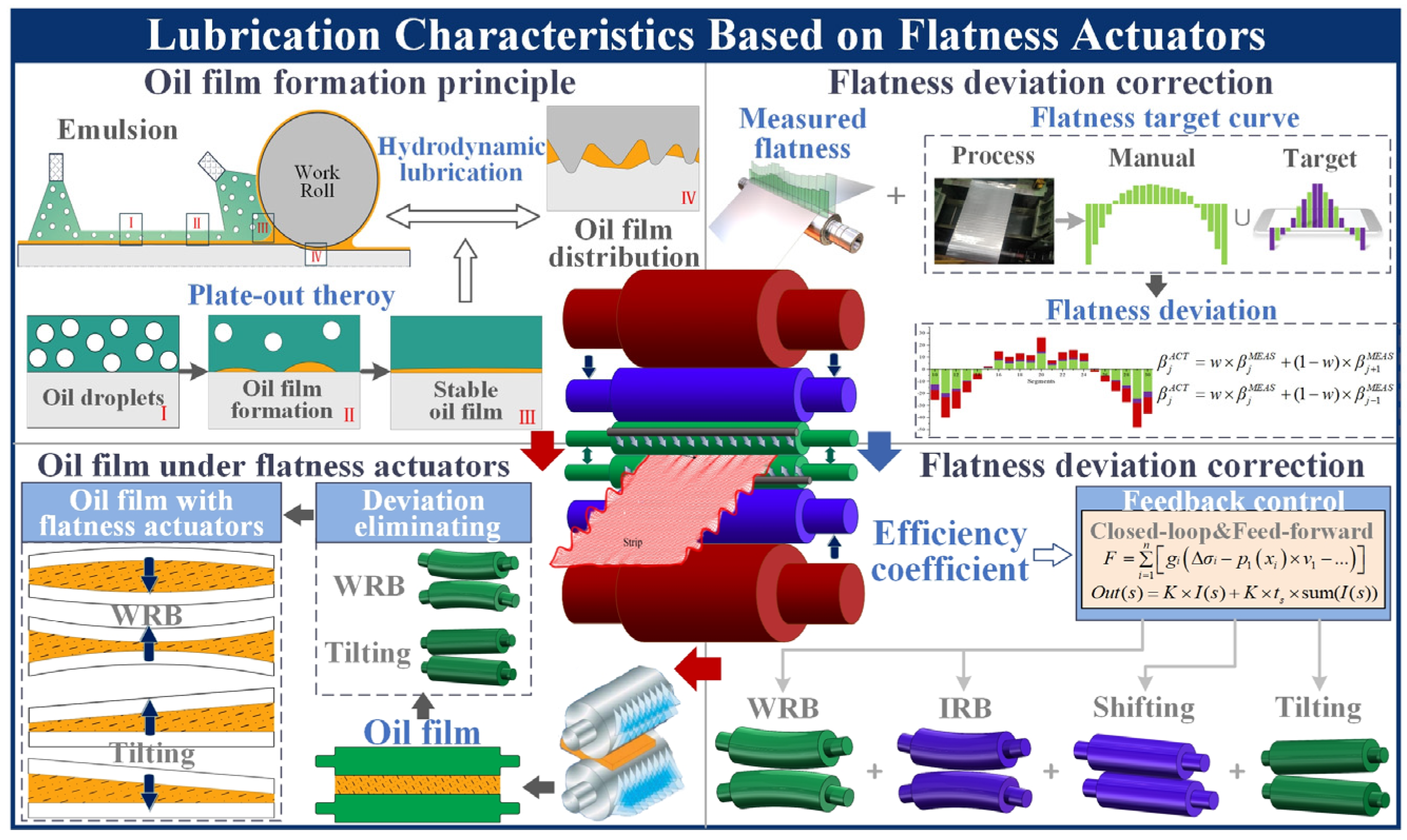
Work roll bending and tilting roll by adjusting the roll surface convexity and roll surface contact angle, respectively, making the change in the profile of the loaded roll gap and online dynamic correction of the flatness, but also affects the lubricant distribution characteristics in the loaded roll gap, and thus changes the lubrication characteristics [10]. The lubrication characteristic of cold strip rolling based on flatness actuators is shown in Figure 1.
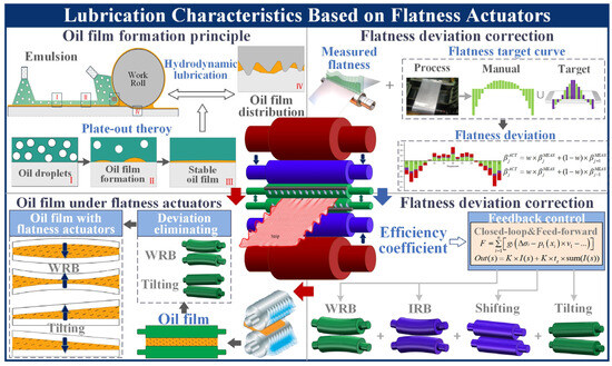
Figure 1.
The cold strip rolling process is based on flatness actuators and lubrication.
The lubrication characteristics directly affect the setting accuracy of key rolling process parameters, especially the rolling force of the final stand with flatness dynamic correction [11]. In the rolling force equation mentioned by Lv et al. [12], the accuracy of the calculated results is affected by the lubrication status factor (LSF). The coefficient of friction is a critical parameter in determining the LSF.
It was found that the lubrication status factor was mismatched with the actual lubrication characteristics in the production research, resulting in a significant deviation between the measured and setting rolling force [13,14]. Therefore, it is an urgent challenge for many enterprises to obtain accurate information on lubrication status to optimize the lubrication status-related parameters for the rolling force calculation in the final stand.
Scholars improve the accuracy of the lubrication status factor by optimizing the coefficient of friction (COF). The most basic way to obtain the COF is the mechanical calculation method, i.e., the COF is obtained by dividing the friction stress measured on the strip surface by the corresponding rolling pressure [15]. Some scholars obtained the setting equation of COF through the combination of rolling theory and lubrication characteristics [16,17]. Also, some scholars got the COF by simulating cold rolling experiments directly [18,19].
However, the current method for obtaining the COF only discusses the effects of rolling characteristics such as reduction, strip width, tension, etc. It neglects the influence of the flatness actuators on the lubrication state. In addition, the theoretical calculation method makes more assumptions, and the experiment methods still deviate from the actual rolling conditions.
The emergence of AI (artificial intelligence)-based optimization methods provides the possibility of further clarifying the hidden relationship between various data types. It has been widely used in the optimization of rolling process parameters optimization for cold strip rolling [20,21]. Optimization of the strip gauge and shape for cold strip rolling can be achieved by the deep neural network method, improving the product quality and efficiency of production [22]. Bu et al. [23] optimized the bending roll force setting model using a multi-objective optimization method to achieve decoupled control between the bending roll and rolling force. Wang et al. [24] improved the accuracy of the coolant output for selective work roll cooling control system by a volution-gray wolf algorithm optimization support vector machine regression.
Therefore, synthesizing the lack of research on the LSF, this paper takes the high-order flatness target in Jin et al. [25] as the basis and considers the influence of the work roll bending and tilting roll in flatness actuators on the lubrication characteristics during strip rolling. This paper then combines this with the current status on the application of the AI-based optimization method in the cold strip rolling, taking the UCM six-roll and five-stand tandem cold rolling mill as the platform and establishing the optimization method of the LSF for the final stand. The accuracy and application value of the proposed method are verified by the rolling force setting accuracy and after-rolling gauge characteristics. The contributions of this paper are as follows:
- Based on the high-order flatness target, the online flatness deviation correction model for the intermediate roll bending, work roll bending, and tilting roll has been established by considering the influence of the rolling process parameters and the different flatness actuators and has been applied to the rolling production;
- Based on the Reynolds equation and the oil film thickness characteristics in the inlet zone, a model for characterizing the instantaneous oil film thickness at any position in the work zone according to the profile of the loaded roll gap has been derived;
- Based on the symbolic regression, the relationship between the LSC and the instantaneous oil film thickness, work roll bending, and tilting roll in the rolling force model of the final stand is established, and the influence of each variable on the LSC is revealed;
- The research method in the paper can ensure that the setting value of the rolling force in the final stand is closer to the actual rolling state and can improve the accuracy of the strip gauge.
The other parts of the paper are as follows: Section 2 introduces the theoretical models developed and needed in the paper, including the flatness correction model of the flatness actuators and the instantaneous oil film thickness model; Section 3 describes the fundamentals, structure, and evaluation of the analytical methods adopted in the paper; Section 4 shows the results of the innovative analytical method via samples, the relationship between the variables and the impact of the analytical results on the critical quality indicators; Section 5 summarizes the research findings, results, and implications on cold rolling production, it also discusses future research directions regarding the content of the paper.
2. Calculation Model
2.1. Flatness Actuators Setting Model
Jin et al. [25] proposed a flatness target-setting method with high-order flatness characteristics. This method increased the number of flatness measurement sensors to refine the flatness measurement results. Thus, an innovative flatness deviation correction should correspond to the new flatness target in the flatness actuators.
Due to the close contact between the rolls, the flatness actuators also interact with each other. Rolling force, strip width, and other vital rolling parameters will also affect the adjusting effect of the flatness actuators on the flatness quality. Therefore, this section establishes an online correction model for flatness deviation of the intermediate roll bending, work roll bending, and tilting roll based on the mutual influence between the flatness actuators and the influence of related rolling process parameters.
First, the quadratic influence sub-coefficients and quadratic influence coefficients based on , , , and are established.
When establishing the influence coefficients, they are all expressed as a quadratic order structure concerning the symmetry characteristics of the flatness target.
(1) Establish quadratic influence sub-coefficients considering , , , and :
where is the identifier of the type of flatness actuators and can be work roll bending, intermediate roll bending, and tilting roll; is the variable for and , , , ; , , and are the constant term coefficient, primary term coefficient, and quadratic coefficient, respectively, of .
(2) Establish quadratic influence coefficients based on :
where is the compensation coefficient.
Next, the flatness deviation correction coefficient is established based on the high-order flatness target:
where are computation coefficients and are queried from the flatness control server; is the normalized position of the strip in the wide direction; is the number of the measured section in the setting of the flatness target; and are the start and end positions of the measured segment in the flatness target, respectively; , , and are all obtained by Jin et al. [25]; is the composite coefficient and is expressed as follows:
where is the self-learning coefficient generated by the self-learning algorithm in the flatness control server; is the control mode coefficient obtained from the basic-level control system.
Lastly, the flatness deviation correction models of roll bending and tilting roll are established by considering the mutual influence of each flatness actuator:
where is the flatness deviation at the jth measured segment; , , and are the gain coefficients of the corresponding flatness actuators.
2.2. Instantaneous Oil Film Thickness in Work Zone
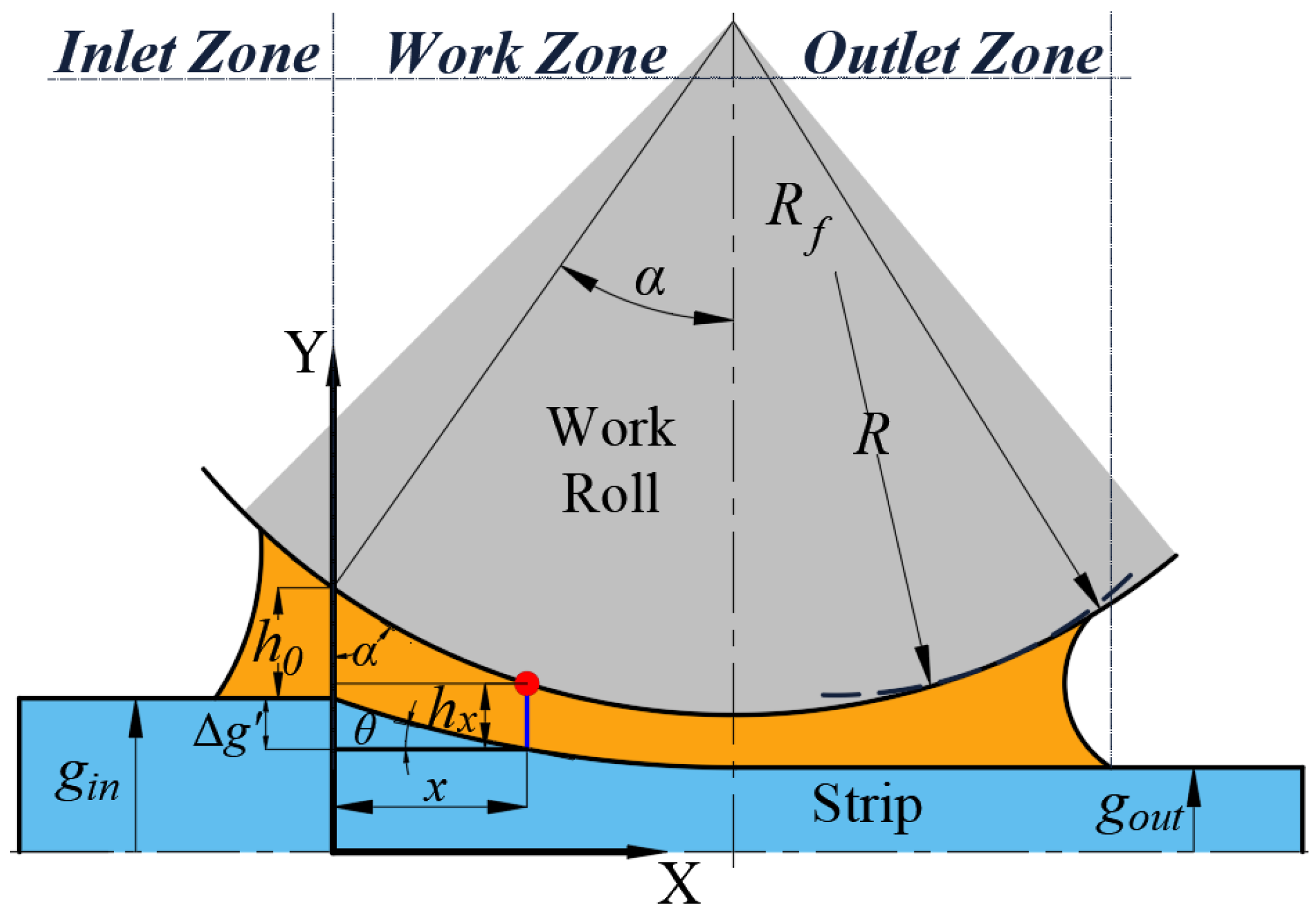
The oil film profile in the work zone coincides with the loaded roll gap characteristics based on the fluid characteristics with sufficient lubrication [26]. Figure 2 shows the distribution characteristics of lubricant in the loaded roll gap under ideal lubrication characteristics in cold strip rolling.

Figure 2.
Distribution characteristics of the lubricant in the loaded roll gap.
Assume that the oil film thickness at any position in the work zone is a linear function of position , as shown in Figure 2, and denote as follows:
Based on the Reynolds equation, the pressure distribution equation of the oil film in the work zone can be expressed as follows [27]:
The instantaneous viscosity of the lubricant at oil film pressure is as follows [28]:
is defined as a dimensionless parameter and denoted as follows:
Equation (8) is taken into the right-hand side of Equation (9):
Equation (12) is integrated and yields the following:
At the boundary of the working zone, is zero, assuming that the oil film pressure gradient is negligible [29]. The result of taking derivatives on both sides of Equation (11) and Equation (10) is carried forward to Equation (13):
Let be, respectively:
Then Equation (14) can be expressed as follows:
The expression for concerning is obtained based on Equation (8) and brought to in Equation (15):
It can be obtained based on Equation (18):
Equation (8) is transformed into the form of a quadratic term and brought to in Equation (15):
Equations (19) and (21) are integrated over and , respectively, and yield:
Then, can be expressed as follows:
where
Based on boundary condition #1: , , . can be expressed as follows:
Based on the Tresca criterion [30], boundary condition #2: , , , then the following occurs:
where in Equation (27) is as follows:
Then, can be expressed as follows:
Therefore, the expression for the dynamic oil film thickness in the work zone is as follows:
2.3. Lubrication Status Factor
The widely adopted rolling force model in cold strip rolling can be expressed as follows [31]:
where , , , , and relative parameters, respectively, are as follows:
The and in Equation (35) are only related to the rolling schedule and remain constant during the rolling of a strip coil. is the elastic deformation of the work roll due to the high pressure. Simulations have shown that the difference between and is not enough to affect the strip rolling process significantly, and some scholars have directly adopted for the calculation of rolling parameters [32,33]. Hence, becomes the only variable in Equation (35). Moreover, a 0.1 change in the value of results in the change of tens of tons in Equation (31).
The lubricant status decisively influences the during the rolling process. The smaller the , the better the lubrication and the corresponding value will be reduced. Moreover, only five variables are included in Equation (31), and the relationship between the variables is multiplicative. Therefore, it is reasonable and efficient to optimize and analyze the directly to obtain a more accurate rolling force.
In the present study, can be called the “stress status coefficient” or “friction status coefficient.” However, the significant change of is mainly caused by the lubrication status. Therefore, in this paper, is named as “lubrication status factor (LSF)”.
3. AI-Based Optimization Methods Modeling
3.1. Symbolic Regression
Symbolic regression is a regression analysis method based on genetic algorithms, revealing potential relationships between data and generating explicit representation equations by simulating the evolutionary process [34,35]. The basic principle of symbolic regression can be expressed as follows:
where is the objective variable; is the optimization coefficient; is the set consisting of all the objective variables; is the set of basis functions containing all the possible functional equations during the execution of the symbolic regression process; is the error term, reflecting the gap between the predicted value and the actual value; is the total number of basic functions. and can be denoted, respectively, as follows:
where to are target variables; is the number of target variables; is the predicted value.
The set of computational laws in symbolic regression can be expressed as follows:
In symbolic regression, the arithmetic rules need to be adjusted in real time based on the optimization condition and validation analysis to achieve efficient and accurate analysis results.
3.2. Analysis Structure
The tree structure is used to characterize the execution process of the algorithm in symbolic regression based on genetic algorithms. The tree structure naturally represents mathematical expressions and facilitates genetic operations with high flexibility and scalability [36]. In the execution process, the following occurs.
First, some individuals from the current population are selected as iterative objects based on the fitness value of the alternative function to obtain higher population quality and faster evolutionary efficiency. Second, the computational rules, by combining the two parents, keep the better characteristics of the parent individuals and thus generate diversity, contributing to finding the optimal solution faster in the search space. Finally, new computational rules are introduced during the iteration process to increase the diversity of the population and prevent the population from falling into local optimal solutions, thus improving the global search capability of the symbolic regression. The analysis procedure of symbolic regression based on the genetic algorithm is shown in Figure 3.
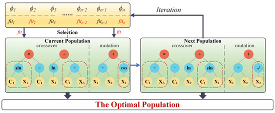
Figure 3.
Symbolic regression based on genetic algorithm.
3.3. Target Variables and Pre-Processing
Work roll bending and tilting rolls affect the profile of the loaded roll gap, changing the distribution characteristics of the lubricant between them and, thus, the lubrication status [37,38]. Therefore, the value of work roll bending and roll tilting are taken as two important variables for analyzing the LSF and denoted as and , respectively. Both and consist of the setting value, the manually adjusted value, and the result of Equation (5) or Equation (7) corresponding to the work roll bending or tilting roll.
The oil film thickness directly determines the lubrication status during cold strip rolling. Therefore, the instantaneous oil film thickness is taken as the third variable that determines the LSF and is calculated by Section 2.2 [39]. can be expressed as follows:
Since the length unit and the mechanical unit belong to different categories of physical quantities, the value of the work roll bending can reach hundreds of kilonewtons, and the value of the tilting roll and the oil film thickness may be only a few micrometers, it will significantly affect the analysis results. Therefore, the variables must be standardized and converted into dimensionless parameters with the same data characteristics. The method of standardization can be expressed as follows:
where ; and are, respectively, the minimum and maximum values of .
3.4. Evaluation Strategy
This paper employs self-evaluation and comparative evaluation. Self-evaluation verifies the accuracy of the prediction results by analyzing the trend agreement and error distribution of the prediction results with the test results. Comparative evaluation validates the effectiveness and applicability of the adopted AI-based analytics in a specific data application environment by comparing different categories of AI-based analytics and other analytics techniques within the same category.
For self-evaluation, the analyzed data are displayed through scatter plots or line graphs, allowing an intuitive and clear presentation of the data trends over time; for the error distribution, the classical frequency distribution histogram is adapted to display the distribution characteristics of the prediction error.
For the comparative evaluation, Root Mean Square Error (RMSE) is more sensitive to larger errors and can identify extreme errors in the model in some cases [40]. Mean Absolute Error (MAE) does not amplify the effect of large errors and makes the evaluation metrics easier to interpret, responding to the average gap between the predicted and the actual values [41]. Mean Absolute Percentage of Error (MAPE) facilitates comparisons of the data on different scales [42]. Therefore, RMSE, MAE, and MAPE were chosen as the evaluation criteria for the comparative evaluation and can be expressed, respectively, as follows:
where and are the measured and predicted values of the data in the th group, respectively; is the total group numbers of collected data.
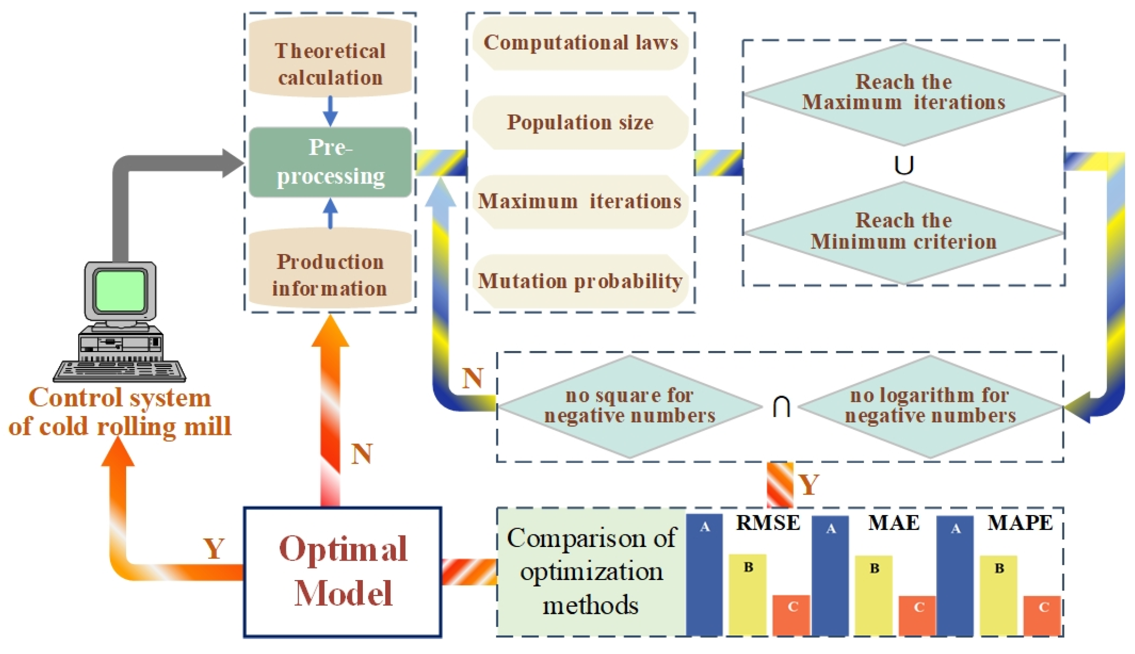
The steps in the optimization analysis of the lubrication status factor are as follows and shown in Figure 4:
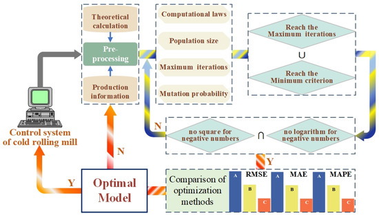
Figure 4.
The optimization architecture of the lubrication status coefficient.
- Extract or compute the training data for selected variables and implement preprocessing for the training data;
- Establish the symbolic regression analysis architecture based on the genetic algorithm, determine initial values for the number of populations, the maximum number of iterations, and the variation probability in the architecture, and formulate the initial law of calculation;
- The analysis results are obtained when the number of iterations reaches the maximum value or the fitness reaches the required value;
- Adjust the maximum number of iterations and the optimal fitness threshold based on the results of Step 3 and adjust the law of calculation by analyzing the function structure of the results;
- Check the function’s structure to ensure no structure for logarithms and squares for negative numbers;
- Repeat Step 3 to Step 5 until the optimum analysis result is obtained;
- Select several optimization methods in the same and different categories as symbolic regression and show the applicability of the selected analysis results by RMSE, MAE, and MAPE;
- The influence of the variables in the optimization results on the analytical objectives is analyzed by single-factor analysis.
4. Analysis and Applications
4.1. Results and Analysis
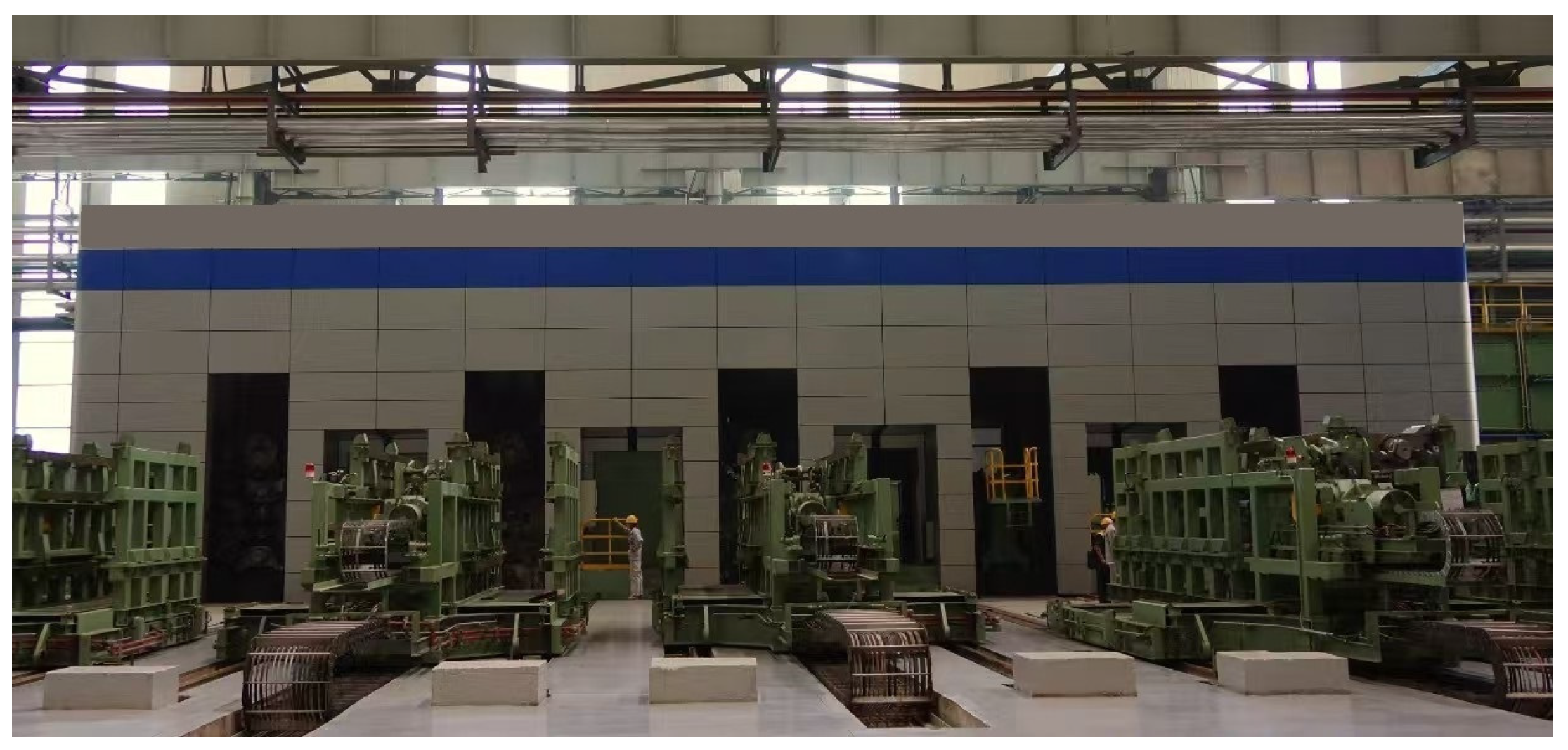
This paper analyzes and validates the study using the 1450 mm UCM six-roll, five-stand tandem cold rolling mill, whose structure is shown in Figure 5.
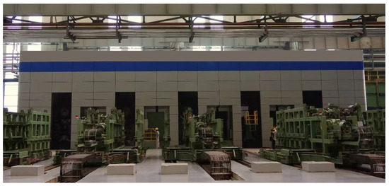
Figure 5.
1450 mm UCM six-roll, five-stand tandem cold rolling mill.
This mill has five flatness control mechanisms: work roll bending roll, intermediate roll positive bending roll, intermediate roll traverse and roll tilting, and segmented cooling. The work roll bending and roll tilting were selected for analysis in this study. The main parameters of the equipment are shown in Table 1.

Table 1.
The basic information about the mill.
The rolling process of a strip oil can be divided into five stages based on the rolling speed characteristics, namely, the head stage, the accelerating stage, the uniform rolling stage, the decelerating stage, and the tail stage, as shown in Figure 6 [43]. Since factors such as the non-uniformity of material properties in the head and tail can affect the accuracy of the analysis, only accelerating, decelerating, and uniform rolling processes were selected for the study, and the accelerating and decelerating phases were combined into the non-uniform rolling stage.
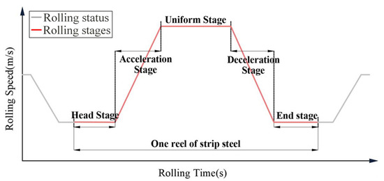
Figure 6.
Characterization of rolling stages based on rolling speed.
For the symbolic regression in this study, the data of the work roll bending and tilting roll are derived from the measured values of the flatness control system in this experimental platform, and this flatness control system utilizes , , and in Section 2. The oil film thickness employs the computed value in Section 2.
, and should be verified based on the mill’s ability to adjust the flatness deviation and the after-rolling flatness standard deviation. When the measured values of , and , meet the corresponding control ranges in Table 1, it can be considered that the control ability of the mill on flatness deviation is satisfied. The flatness standard deviation requires that the average value does not exceed 9 I-Unit and the efficiency is greater than 95.4%. In cold strip rolling, the oil film’s thickness is difficult to obtain online, and most scholars investigate this by experimental methods. Therefore, the classical formula derived by Wilson et al. [44] is used to compare with the presented calculation to verify the validity of the oil film thickness model in the paper.
The validation results for Section 2 are shown in Figure 7. From Figure 7a,b, the measured values of the intermediate roll bending (both sides) are distributed around 215 kN, much smaller than the limit value of 1000 kN; the measured distribution of the work roll bending is from 440 kN to 520 kN, smaller than the limit value of 720 kN. The maximum value of tilting rolls is 0.29 mm, less than the limit value of 1.5 mm. Therefore, it can be concluded that the calculation results of , and are valid. From Figure 7c, the flatness standard deviation distribution is from 5.1 I-Unit to 6.7 I-Unit, smaller than the process standard and with an efficiency of 100%. From Figure 7d, the oil film thickness calculation results mentioned in this paper are slightly larger than the formula of Wilson et al. [44], and the calculation error is only in the range of 0.09 μm to 0.15 μm, with a good agreement of the calculation results and proving the validity of the oil film thickness calculation method in this paper.

Figure 7.
The validation results for bending rolls, tilting roll, and oil film thickness: (a) Work roll bending and intermediate roll bending; (b) Tilting roll; (c) Flatness standard deviation; (d) Oil film thickness calculation error analysis by comparing the results of Wilson et al. [44].
The method in Section 3 was used to analyze and optimize the data for the uniform and non-uniform rolling stages, respectively. The symbolic regression based on the genetic algorithm has seven key setting parameters:
- Computational rules. Computational laws define the operators and algorithms available in symbolic regression and are determined by the nature of the data and the context of the problem, directly affecting the search space of symbolic regression. A restricted computational law can prevent the model from capturing the complex patterns of the data, and a broad computational law can lead to excessive computational overhead and overfitting;
- Population size. The population size indicates the number of candidate solutions used for selection, crossover, and mutation in each generation, and the choice is based on a combination of computational cost and search capability. A too-small population tends to cause the optimization model to fall into a local optimum solution, and a too-large population leads to slower convergence of the optimization model;
- Maximum number of iterations. The maximum number of iterations is the maximum number of optimizations that can be performed and is chosen based on the complexity of the data and computational resources. Too few iterations can leave the search unfinished and miss the best solution, and too many iterations can lead to over-computation and waste of resources;
- Crossover. Crossover is the generation of new individuals by combining the expression structures of two-parent individuals. In symbolic regression, crossover usually generates new expressions by swapping certain subtrees of the parents. Crossover patterns can affect the algorithm’s ability to jump in the search space, and poor choices may result in expressions of the child individuals being too similar, leading to a loss of diversity and thus affecting the optimization process;
- Mutation. Mutation is the process of increasing the diversity of the search space by randomly modifying some part of the mathematical expression represented by the mutation probability. The mutation probability controls the likelihood that each individual will make a mutation. Mutation probability is generally low to prevent too frequent random changes from destroying existing good genes; too low a mutation probability tends to make the model converge prematurely, and too high a mutation probability can lead to too random a search process and loss of convergence;
- Training set ratio. The training set ratio refers to the proportion of data selected from the overall data set for model training, generally 70% to 80% of the total data set. Too small a training set ratio will cause the optimization model to be under fitted and unable to learn the full picture of the data, while too large a training set ratio will cause the model to overfit the training data and reduce its prediction ability for new data;
- Test set ratio. The proportion of the test set refers to the appropriate proportion of data from the total data set used to test the model effect; the test set does not participate in the training of the model and is only used to evaluate the performance of the model, generally 20% to 30% of the total data set. Too small a test set will lead to unreliable evaluation results and fail to accurately reflect the generalization ability of the model, while too large a test set will lead to insufficient training data and affect the learning effect of the model.
The setting results of the key parameters in the optimization method are shown in Table 2.
Table 2.
The key parameters of the optimization method.
The central processing unit (CPU) of i9-13900 and random access memory (RAM) of 32 GB served as the hardware environment for the optimization process. For the software, the optimization method was implemented in Python 3.11, and Pandas 2.1.3 and NumPy 1.26.4 libraries were used to support the pre-processing and analysis of the dataset.
Overfitting is a common model generalization capability flaw in regression-based predictive analytics, reflecting the relationship between the model and the data, particularly the balance between model complexity and data characteristics. Overfitting usually indicates that the model overlearns the details and noise in the training data and fails to learn more general laws that can be generalized to new data. In this paper, we take the following steps to avoid overfitting as much as possible:
- Selection and processing of analyzed data: Since the calculation in Section 2 has included key basic rolling information such as thickness, width, and instantaneous viscosity of the lubricant and is centered on the research theme of this paper, the analyzed variables are only selected as oil film thickness, work roll bending, and tilting roll, to avoid the coupling between the variables and the occurrence of the overfitting phenomenon. Based on the on-site investigation, a few outliers were also eliminated to ensure the consistency of the data characteristics;
- Parameter setting of the analytical model: select the universal and representative algorithms. Meanwhile, the initial value of the model parameters is set to the value that can be obtained with higher accuracy and less overfitting according to the research experience of scholars [45], and some parameters are adjusted appropriately to improve the accuracy of the analysis based on the unique data characteristics in this paper;
- Validation of analysis results: data other than the training and validation sets are added to validate the accuracy of the results and the prediction trends and to check whether the model has an overfitting trend.
Due to the randomness of individual generations within the population, the results differed for each run. After several runs, the prediction results with optimal accuracy and reasonable function structure were selected. The prediction results for the uniform and non-uniform rolling stages are shown in Equations (48) and (49), respectively, and the corresponding tree structures are shown in Figure 8 and Figure 9, respectively.
where and are the optimized LSFs for the uniform and non-uniform rolling stages, respectively.
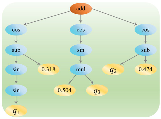
Figure 8.
Tree structure for the analyzed results of the uniform rolling stage.
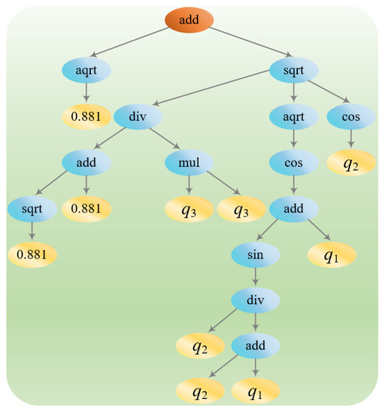
Figure 9.
Tree structure for the analyzed results of the non-uniform rolling stage.
Therefore, the optimized Equation (31) can be characterized as follows:
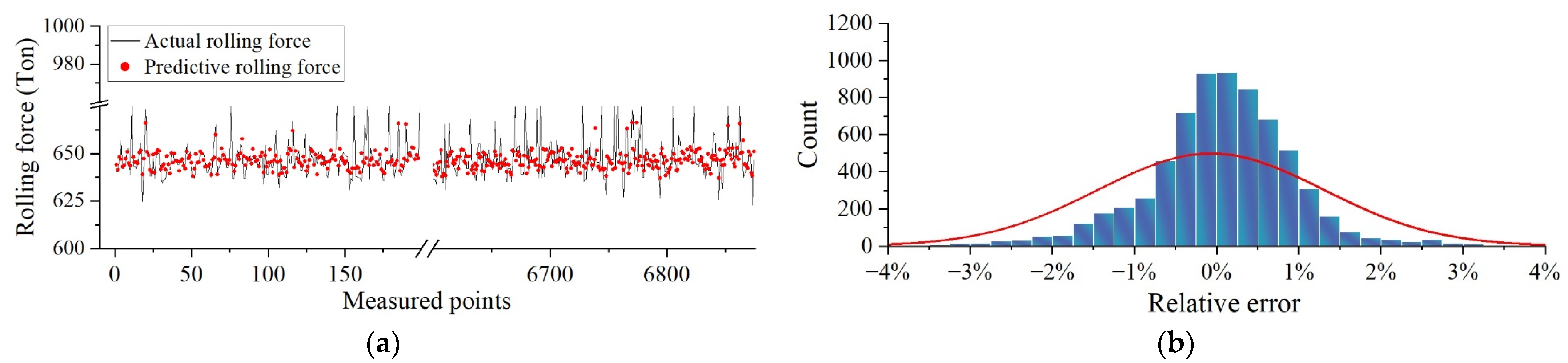
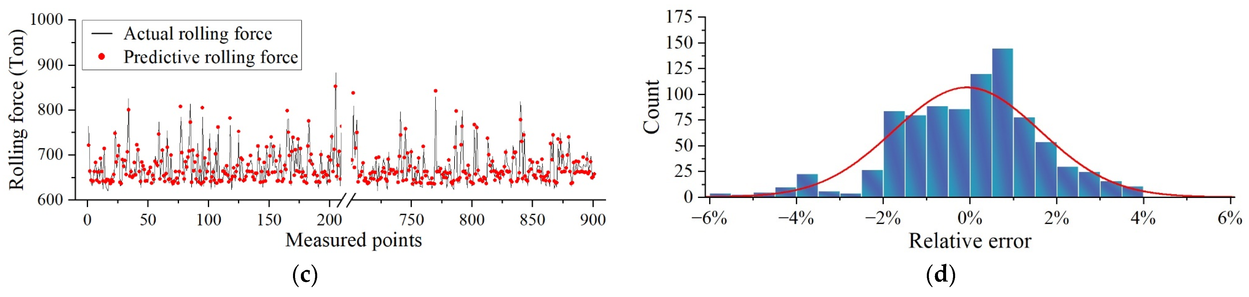
The predicted trends and their corresponding frequency distribution histogram are shown in Figure 10. From the trend analysis plots in Figure 10a,c, the predicted results are consistent with the trend of the actual values. From the frequency distribution histograms in Figure 10b,d, the overall error of prediction for the uniform rolling stage is within ±3%, and most of the data are within ±1.5% of the prediction error; the overall error of prediction for the non-uniform rolling stage is within ±4 and is between ±2% for most of the data and around 6% for a few.

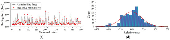
Figure 10.
The trend of the analyzed results and the corresponding frequency distribution of the error: (a) The trend of optimization results in the uniform rolling stage; (b) The frequency distribution of the error in the uniform rolling stage; (c) The trend of optimization results in the non-uniform rolling stage; (d) The frequency distribution of error in the non-uniform stage.
The prediction results’ trend and error distribution characteristics show that the analyzed results have good accuracy and that the uniform stage is better than the non-uniform stage. That’s because the key process features in the uniform rolling stage are more stable, making the analyzed data have obvious regularity. In contrast, the key process features in the non-uniform rolling stage are less stable, resulting in less regularity of the analyzed data.
To verify the superiority of symbolic regression in the application background of the analyzed data, two categories of optimization methods containing Deep Neural Networks (DNNs), Support Vector Machines (SVMs), and traditional Multiple Linear Regression were selected and compared by RMSE, MAE, and MAPE. The key parameters in the DNNs and SVMs are shown in Table 3, and the least squares method was used for Multiple Linear Regression.
Table 3.
The key parameters in the comparison model.
The comparison results in Figure 11 show that, in the uniform rolling stage, the RMSE and MAPE of symbolic regression are superior to the other three methods, but the MAE is slightly weaker than the DNN, and the MAPE is somewhat weaker than the SVM; in the non-uniform rolling stage, all the indexes of symbolic regression are better than the other three optimization methods.
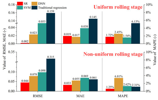
Figure 11.
Performance comparison of comparative analysis by other methods.
In detail, the MAE of the uniform rolling stage is only 0.002 larger than that of the DNN, and the MAPE is only 0.18% larger than that of the SVM. However, these subtle differences are insufficient to differentiate significantly between the two optimization methods. Overall, the analysis results of symbolic regression are superior to several other comparative methods. More importantly, symbolic regression can obtain linear characterization equations, allowing intuitive observation of the influence pattern among the variables on the analysis objectives, which is incomparable to the other three methods.
Only one setting value for the rolling force can be achieved for a strip coil, and most of the production process for a strip coil is in the uniform rolling process. Moreover, based on the analysis of Figure 10, the analysis accuracy of the uniform rolling stage is better than that of the non-uniform rolling stage. Therefore, the setting value of the rolling force is obtained using the uniform rolling stage in Equation (50). Since the poor stability of the accelerating and decelerating rolling stages, the non-uniform rolling stage in Equation (50) is employed to predict occasional abrupt changes in the rolling process and thus avoid the generation of defective products.
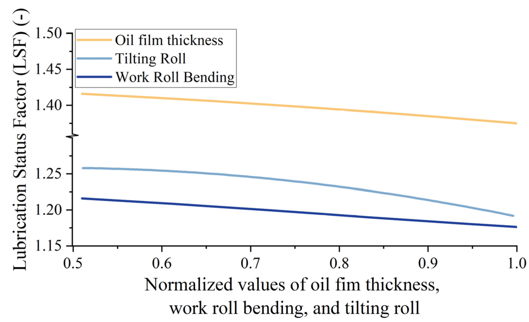
To analyze the influence of flatness actuators on the lubrication status, the impact of oil film thickness, work roll bending, and tilting roll on the LSF was analyzed by single-factor analysis within the appropriate value range. The study’s results are shown in Figure 12.
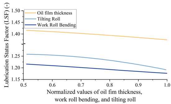
Figure 12.
The trend analysis of the impact of oil film, work roll bending, and tilting roll on LSF.
From Figure 12, it can be seen that the LSF decreases gradually with the increase of oil film thickness, indicating a better lubrication status. This is consistent with the findings of other scholars [46,47] and verifies the accuracy of the physical structure for the optimized LSF’s equation; when the work roll bending and tilting roll are increased, it will make the LSF decrease, meaning that the lubrication effect is better. This is because, according to the hydrodynamic lubrication, the work roll bending and tilting rolls, respectively, increase the deflection of the work roll surface and the angle between the upper and lower work rolls, allowing more lubricant to fill the loaded roll gap, enhancing the lubrication effect and thus reducing the value of .
4.2. Experimental Validation
To indicate the practical application value of the optimization results, strips with target sizes of (width 970 mm, gauge 0.23 mm) and (width 973 mm, gauge 0.199 mm) were used to apply the optimization results and to explore the characteristics of their influence on product quality. The two strips are named Type 1 and Type 2, respectively.
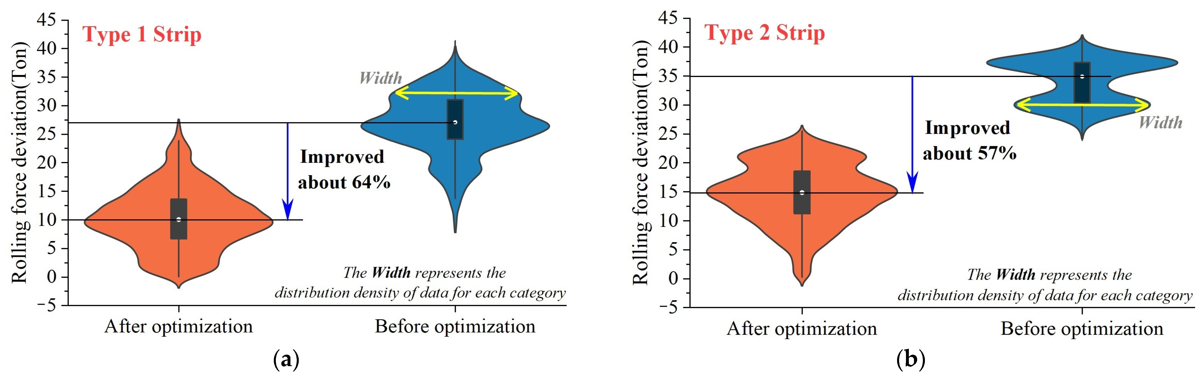
The calculation accuracy of the rolling force for the sample strips is compared in Figure 13. As shown in Figure 13, before optimization, the difference between the setting and the actual value of rolling force for the two types of strips is about 28 tons and 35 tons, respectively; after optimization, only about 10 tons and 15 tons of difference between the setting and the actual value of rolling force for the two types of strips are observed. The accuracy of rolling force prediction has been improved by about 64% and 57%, respectively.

Figure 13.
Comparative analysis of applications based on rolling force errors: (a) Comparison of errors between setting and actual values of rolling force before and after optimization of the Type 1 strip; (b) Comparison of errors between setting and actual values of rolling force before and after optimization of the Type 2 strip.
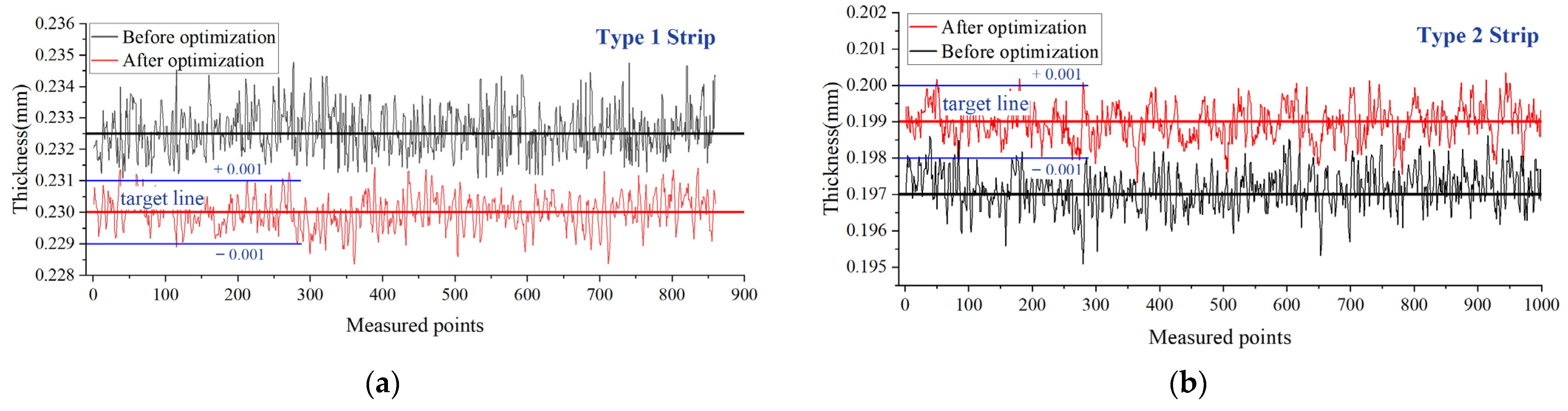
Also, the after-rolling gauge data of the sample coils were collected, as shown in Figure 14. As found in Figure 14, before optimization, the after-rolling gauge of the two type strips fluctuated around 0.2325 mm and 0.197 mm, respectively; after optimization, the after-rolling gauge of the two type strips fluctuated around the target value of 0.23 mm and 0.199 mm, respectively, and the absolute value of fluctuation error is about 0.001 mm.
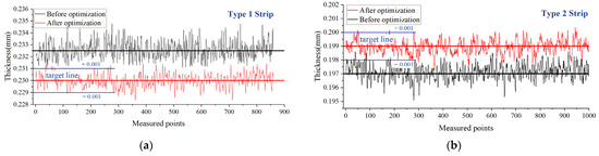
Figure 14.
Comparative analysis of applications based on after-rolling gauge: (a) Comparison of the after-rolling gauge of the Type 1 strip; (b) Comparison of the after-rolling gauge of the Type 2 strip.
The analysis of Figure 13 and Figure 14 shows that the optimized LSF can improve the rolling force setting accuracy and strip gauge index.
To verify the influence trend of work roll bending and tilting on the lubrication status coefficient obtained by the single factor analysis in Section 4.1, the theoretical analysis conclusions were verified experimentally with the rolling force as an observable indicator. Before the experiment, it must ensure the uniform strip material properties, maintain a constant rolling speed, tension, and other crucial rolling parameters, and turn off the work roll bending closed-loop control, tilting roll closed-loop control, flatness feed-forward control, automatic gauge control, and automatic tension control. The experiment scheme is shown in Table 4.
Table 4.
Experimental procedures for analyzing the effects of work roll bending and tilting roll on lubrication characteristics.
As shown from the test results in Figure 15, the measured rolling force decreases when the work roll bending and tilting roll are gradually increased, which is consistent with the trend in Figure 12.
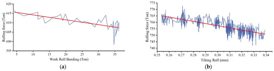
Figure 15.
Experimental analysis of effects of work roll bending and tilting roll on the lubrication state: (a) The experiment result of work roll bending; (b) The experiment result of the tilting roll. (the red lines in (a,b) represent the trend).
According to the hydrodynamic lubrication, this phenomenon can be explained as follows: work roll bending and tilting roll change the roll surface convexity and the tilting angle between the upper and lower work rolls, respectively, enabling more lubricant to enter the loaded roll gap and forming a thicker oil film. The thicker oil film occupies more roll gap space, causing a decrease in strip thickness to ensure that the value of the loaded roll gap remains physically constant.
In other words, a thicker oil film reduces the required rolling force while the target thickness remains constant, which is one reason lubrication improves the mill’s rolling capacity.
5. Conclusions
Lubrication is a key part of the cold strip rolling process and importantly influences the key rolling process parameters such as lubrication status factor, rolling force, and the after-rolling gauge of the strip. This paper deeply analyzes the influence of lubrication characterization parameters on the lubrication status factor in the rolling force model, clarifies the role of flatness actuators’ online dynamic adjustment on the profile of the loaded roll gap and lubrication characteristics, and summarizes the current status of the research on lubrication characterization parameters and its shortcomings. By referring to the application of the AI-based analysis method in cold strip rolling and combining it with the process characteristics of continuous strip rolling, an intelligent optimization method of lubrication status factor in the rolling force model based on the dynamically loaded roll gap characteristics is established adopting the final stand of the UCM six-roll, five-stand tandem cold rolling mill as the research platform, and the following research results are obtained as follows:
- Based on the research results of the high-order flatness target characteristics and considering the mutual influence between each flatness actuator, the flatness deviation correction model of work roll bending, intermediate roll bending, and tilting roll based on the width of the strip, after rolling thickness, rolling force, and intermediate roll transverse shifting is established, and served as the basic data for the AI-based optimization analysis of lubrication status factor;
- Based on the hydrodynamic lubrication and the geometrical characteristics of the loaded roll gap, the geometrical characterization equation of the oil film thickness at any position within the work zone is derived from Reynolds’ equation and also served as the basic data for AI-based optimization analysis of lubrication status factor;
- The pre-treatment method of analyzed data is determined by summarizing and interpreting symbolic regression’s form, principle, and composition. The explicit characterization equations between the lubrication status factor and the oil film thickness, the work roll bending, and the tilting roll are constructed according to the characteristics of the strip rolling process in the uniform rolling stage and the non-uniform rolling stage, respectively;
- The error frequency distribution characteristics discuss the accuracy and superiority of the research results, prediction trend analysis, RMSE, MAE, and MAPE. The influence of the work roll bending and tilting roll in the flatness actuators on the lubrication characteristics in the cold strip rolling is verified by combining the theoretical and experimental analyses. The reasons for the above-influencing characteristics are explained based on the hydrodynamic lubrication.
Meanwhile, the validity of the research results is verified with the application of rolling force and the strip gauge. It is found that the setting accuracy of the rolling force can be improved by about 60%. The quality of the after-rolling gauge can be improved by about 50%, demonstrating that the research method proposed in this paper has a strong application value.
In the traditional setting of rolling procedures, usually, only one characterization method is employed to determine the process parameters under different working conditions. Although these characterization methods consider the influence of closely related parameters, some assumptions can easily lead to a mismatch between the calculation results and the real rolling characteristics. Lubrication during rolling is a process that is very sensitive to the production environment. For example, different rolling speeds can lead to different lubrication characteristics. Therefore, different characterization methods should be established for different production targets and rolling states.
In future research, to further improve the accuracy of the lubrication status factor model, a fine control strategy should be adopted to establish the lubrication status factor equations under different process conditions by categorizing the steel family, width, or thickness of the strip, summarizing all kinds of equations into a database, and incorporating them into the base-level control system.
It is also necessary to introduce the expert setting strategy and add expert correction coefficients in the characterization equations to incorporate special rolling conditions into the setting model and realize the accurate setting of the lubrication status factor under any rolling conditions.
Author Contributions
Conceptualization and Writing—original draft, S.J.; Writing—review and editing and Funding acquisition, X.L., P.W.; Resources and Supervision, X.L., D.Z.; Visualization, F.C.; Methodology, F.L.; Project administration, H.Z. All authors have read and agreed to the published version of the manuscript.
Funding
This research was funded by the National Natural Science Foundation of China, grant number U20A20187; the Natural Science Foundation of Hebei Province, grant number E2024203016; S&T Program of Hebei, grant number 246Z1601G; and Project supported by State Key Laboratory of Featured Metal Materials and Life-cycle Safety for Composite Structures, grant number MMCS20230F07.
Data Availability Statement
Restrictions apply to the availability of these data. Data were obtained from a cooperative company and are available from the corresponding author with the permission of the cooperative company.
Conflicts of Interest
Author Haidong Zhang was employed by the Capital Engineering and Research Incorporation Ltd. The remaining authors declare that the research was conducted in the absence of any commercial or financial relationships that could be construed as a potential conflict of interest.
Nomenclature
| width of strip | mm | |
| target strip gauge | mm | |
| initial strip gauge | mm | |
| reduction | mm | |
| instantaneous reduction | mm | |
| Elastic modulus of work roll | MPa | |
| Poisson ratio of work roll | - | |
| bite angle | rad | |
| the angle based on | rad | |
| change rate of | rad/s | |
| reduction rate | - | |
| Yield stress of strip | MPa | |
| rolling force | kN | |
| the rolling force of the final stand | kN | |
| oil film pressure | MPa | |
| intermediate roll transverse shifting of the final stand | mm | |
| oil film thickness in the work zone | μm | |
| oil film thickness in the inlet zone | μm | |
| change rate of | μm | |
| coefficient of pressure-viscosity | - | |
| initial emulsion viscosity | mm2/s | |
| instantaneous lubricant viscosity | mm2/s | |
| contact arc length | mm | |
| flattening radius of the work roll | mm | |
| radius of work roll | mm | |
| coefficient of friction between strip and work roll | - | |
| coefficient of lubrication factor | - | |
| coefficient of deformation resistance | - | |
| back tension stress | MPa | |
| forward tension stress | MPa | |
| correction of flatness deviation for work roll bending | kN | |
| correction of flatness deviation for intermediate roll bending | kN | |
| correction of flatness deviation for tilting roll | mm |
References
- Ojeda-Lopez, A.; Botana-Galvin, M.; Gonzalez-Rovira, L.; Botana, F.J. Numerical Simulation as a Tool for the Study, Development, and Optimization of Rolling Processes: A Review. Metals 2024, 14, 737. [Google Scholar] [CrossRef]
- Cao, L.; Li, X.; Wang, Q.; Zhang, D. Vibration analysis and numerical simulation of rolling interface during cold rolling with unsteady lubrication. Tribol. Int. 2021, 153, 106604. [Google Scholar] [CrossRef]
- Valigi, M.C.; Malvezzi, M.; Logozzo, S. A Numerical Procedure Based on Orowan’s Theory for Predicting the Behavior of the Cold Rolling Mill Process in Full Film Lubrication. Lubricants 2020, 8, 2. [Google Scholar] [CrossRef]
- Bukvic, M.; Gajevic, S.; Skulic, A.; Savic, S.; Asonja, A.; Stojanovic, B. Tribological Application of Nanocomposite Additives in Industrial Oils. Lubricants 2024, 12, 6. [Google Scholar] [CrossRef]
- Shimura, M.; Kasai, D.; Otsuka, T.; Yamashita, N.; Hirayama, T. Measurement of Oil Film Thickness Distribution in Roll Bite during Cold Rolling Using Quantum Dots. Tetsu-to-Hagane 2023, 109, 865–879. [Google Scholar] [CrossRef]
- Ma, L.; Ma, L.; Lian, J.; Wang, C.; Ma, X.; Zhao, J. Tribological Behavior and Cold-Rolling Lubrication Performance of Water-Based Nanolubricants with Varying Concentrations of Nano-TiO2 Additives. Lubricants 2024, 12, 361. [Google Scholar] [CrossRef]
- Wang, Y.; Li, C.S.; Jin, X.; Xiang, Y.G.; Li, X.G. Multi-objective optimization of rolling schedule for tandem cold strip rolling based on NSGA-II. J. Manuf. Processes 2020, 60, 257–267. [Google Scholar] [CrossRef]
- Sun, W.; Li, J.; Kong, N.; Zhang, J. Flatness defect control during cold rolling of SUS430 stainless steel. Mater. Test. 2024, 66, 896–912. [Google Scholar] [CrossRef]
- Tao, L.; Wang, Q.; Wu, H. Establishment and Numerical Analysis of Rolling Force Model Based on Dynamic Roll Gap. Appl. Sci. 2023, 13, 7394. [Google Scholar] [CrossRef]
- Tieu, A.; Liu, Y.J. Friction variation in the cold-rolling process. Tribol. Int. 2004, 37, 177–183. [Google Scholar] [CrossRef]
- Smmura, M.; Kasai, D.; Otsuka, T. Mechanisms of Slip Generation in Cold Rolling of AHSS. Tetsu-to-Hagane 2023, 109, 377–386. [Google Scholar] [CrossRef]
- Lv, C.; Jiao, Z.J.; Liu, X.H.; Wang, G.D. Hill explicit expression of rolling force taking into consideration elastic deformation of rolled stock. Res. Iron Steel 2000, 3, 32–33+46. [Google Scholar]
- Mercuri, A.; Fanelli, P.; Giorgetti, F.; Rubino, G.; Stefanini, C. Experimental and numerical analysis of roll bending process of thick metal sheets. In Proceedings of the 49th Italian Association for Stress Analysis Conference (AIAS), Genova, Italy, 2–5 September 2020. [Google Scholar]
- Jacobs, L.J.M.; Van Dam, K.N.H.; Wentink, D.J.; De Rooij, M.B.; Van der Lugt, J.; Schipper, D.J.; Hoefnagels, J.P.M. Effect of asymmetric material entrance on lubrication in cold rolling. Tribol. Int. 2022, 175, 107810. [Google Scholar] [CrossRef]
- Le, H.R.; Sutcliffe, M.P.F. A multi-scale model for friction in cold rolling of aluminium alloy. Tribol. Lett. 2006, 22, 95–104. [Google Scholar] [CrossRef]
- Domhof, A.T.M.; Waanders, D.; Hol, J.; Sigvant, M. Friction and lubrication modelling in sheet metal forming: Influence of local tool roughness on product quality. In Proceedings of the 42nd Conference of the International Deep Drawing Research Group (IDDRG), Luleå, Sweden, 19–22 June 2023. [Google Scholar]
- Trzepiecinski, T.; Najm, S.M. Application of Artificial Neural Networks to the Analysis of Friction Behaviour in a Drawbead Profile in Sheet Metal Forming. Materials 2022, 15, 9022. [Google Scholar] [CrossRef] [PubMed]
- Rowe, G.W. Computing the Coefficient of Friction in the Roll Bite from Mill Data. Blast Furn. Steel Plant 1967, 55, 499–508. [Google Scholar]
- Bland, D.R.; Ford, H. The Calculation of Roll Force and Torque in Cold Strip Rolling with Tensions. Proc. Inst. Mech. Eng. 1948, 159, 144–163. [Google Scholar] [CrossRef]
- Zhao, J.W.; Li, J.D.; Qie, H.T.; Wang, X.C.; Shao, J.; Yang, Q. Predicting flatness of strip tandem cold rolling using a general regression neural network optimized by differential evolution algorithm. Int. J. Adv. Manuf. Technol. 2023, 126, 3219–3233. [Google Scholar] [CrossRef]
- Lee, S.H.; Song, G.H.; Lee, S.J.; Kim, B.M. Study on the improved accuracy of strip profile using numerical formula model in continuous cold rolling with 6-high mill. J. Mech. Sci. Technol. 2011, 25, 2101–2109. [Google Scholar] [CrossRef]
- Li, J.D.; Wang, X.C.; Zhao, J.W.; Yang, Q.; Qie, H.T. Predicting mechanical properties lower upper bound for cold-rolling strip by machine learning-based artificial intelligence. ISA Trans. 2024, 147, 328–336. [Google Scholar] [CrossRef]
- Bu, H.N.; Zhou, H.G.; Yan, Z.W.; Zhang, D.H. Multi-objective optimization of bending force preset in cold rolling. Eng. Comput. 2019, 36, 2048–2065. [Google Scholar] [CrossRef]
- Wang, P.F.; Deng, J.K.; Li, X.; Hua, C.C.; Su, L.H.; Deng, G.Y. A novel strategy based on machine learning of selective cooling control of work roll for improvement of cold rolled strip flatness. J. Intell. Manuf. 2024, 35, 3559–3576. [Google Scholar] [CrossRef]
- Jin, S.R.; Li, X.; Wang, P.F.; Li, X.H.; Zhang, D.H. Research and application of the flatness target curve discrete dynamic programming based on two-dimensional decision making. Expert Syst. Appl. 2024, 256, 124947. [Google Scholar] [CrossRef]
- Fu, K.; Zang, Y.; Gao, Z.Y. Partial Film Lubrication Characteristics of Inlet Zone in Cold Strip Rolling. J. Tribol.-Trans. ASME 2014, 136, 041502. [Google Scholar] [CrossRef]
- Patir, N.; Cheng, H.S. An Average Flow Model for Determining Effects of Three-Dimensional Roughness on Partial Hydrodynamic Lubrication. J. Lubr. Technol. 1978, 100, 12–17. [Google Scholar] [CrossRef]
- Pawelski, H. An analytical model for dependence of force and forward slip on speed in cold rolling. Steel Res. Int. 2003, 74, 293–299. [Google Scholar] [CrossRef]
- Wang, Q.Y.; Zhang, Z.; Chen, H.Q.; Guo, S.; Zhao, J.W. Characteristics of unsteady lubrication film in metal-forming process with dynamic roll gap. J. Cent. South Univ. 2014, 21, 3787–3792. [Google Scholar] [CrossRef]
- Heidari, A.; Forouzan, M.R.; Niroomand, M.R. Development and evaluation of friction models for chatter simulation in cold strip rolling. Int. J. Adv. Manuf. Technol. 2018, 96, 2055–2075. [Google Scholar] [CrossRef]
- Li, J.D.; Wang, X.C.; Yang, Q.; Guo, Z.; Song, L.B.; Mao, X. Rolling force prediction in cold rolling process based on combined method of T-S fuzzy neural network and analytical model. Int. J. Adv. Manuf. Technol. 2022, 121, 4087–4098. [Google Scholar] [CrossRef]
- Li, L.; Matsumoto, R.; Utsunomiya, H. Experimental Study of Roll Flattening in Cold Rolling Process. ISIJ Int. 2018, 58, 714–720. [Google Scholar] [CrossRef]
- Wang, H.; Guo, W.; Li, Y.L.; Chen, F.; Wen, J.; Yu, M.; Wang, F.Q. Research on Level 2 Rolling Model of Tin Plate Double Cold Reduction Process. In Proceedings of the Materials Processing Fundamentals Symposium Held at the TMS Annual Meeting and Exhibition, San Antonio, TX, USA, 10–14 March 2019; Springer: Cham, Switzerland, 2019; pp. 131–139. [Google Scholar]
- Makke, N.; Chawla, S. Interpretable scientific discovery with symbolic regression: A review. Artif. Intell. Rev. 2024, 57, 2. [Google Scholar] [CrossRef]
- Engle, M.R.; Sahinidis, N.V. Deterministic symbolic regression with derivative information: General methodology and application to equations of state. AlChE J. 2022, 68, e17457. [Google Scholar] [CrossRef]
- Zhang, H.Z.; Zhou, A.; Qian, H.; Zhang, H. PS-Tree: A piecewise symbolic regression tree. Swarm Evol. Comput. 2022, 71, 101061. [Google Scholar] [CrossRef]
- Song, C.N.; Cao, J.G.; Sun, L.; Tan, X.Y.; Xia, W.H.; Sun, S.T. A multi-stand work roll bending and shifting approach for profile contour and flatness control of electrical steel in multi-width schedule-free rolling using NSGA-II algorithm. J. Manuf. Processes 2024, 120, 895–910. [Google Scholar] [CrossRef]
- Wang, P.F.; Zhang, D.H.; Li, X.; Zhang, W.X. Research and Application of Dynamic Substitution Control of Actuators in Flatness Control of Cold Rolling Mill. Steel Res. Int. 2011, 82, 379–387. [Google Scholar] [CrossRef]
- Fujita, N.; Kimura, Y. Influence of Plate-out Oil Film on Lubrication Characteristics in Cold Rolling. ISIJ Int. 2012, 52, 850–857. [Google Scholar] [CrossRef]
- Chai, T.; Draxler, R.R. Root mean square error (RMSE) or mean absolute error (MAE)?—Arguments against avoiding RMSE in the literature. Geosci. Model Dev. 2014, 7, 1247–1250. [Google Scholar] [CrossRef]
- Mendo, L. Estimation of a Probability with Guaranteed Normalized Mean Absolute Error. IEEE Commun. Lett. 2009, 13, 817–819. [Google Scholar] [CrossRef]
- Elkatatny, S.; Al-AbdulJabbar, A.; Abdelgawad, K. A New Model for Predicting Rate of Penetration Using an Artificial Neural Network. Sensors 2020, 20, 2058. [Google Scholar] [CrossRef] [PubMed]
- Bu, H.N.; Yan, Z.W.; Zhang, D.H. A novel approach to improve the computing accuracy of rolling force and forward slip. Ironmak Steelmak 2019, 46, 269–276. [Google Scholar] [CrossRef]
- Wilson, W.R.D.; Chang, D.F. Low speed mixed lubrication of bulk metal forming processes. J. Tribol.-Trans. ASME 1996, 118, 83–89. [Google Scholar] [CrossRef]
- Trzepiecinski, T.; Lemu, H.G. Improving Prediction of Springback in Sheet Metal Forming Using Multilayer Perceptron-Based Genetic Algorithm. Materials 2020, 13, 3129. [Google Scholar] [CrossRef]
- Lee, R.T.; Yang, K.T.; Chiou, Y.C. Mixture Lubrication with Emulsions in Cold Rolling. Tribol. Trans. 2016, 59, 748–757. [Google Scholar] [CrossRef]
- Li, X.J.; Cui, Y.Y.; He, Z.L.; Bai, Z.H. Model and influence factors of oil film thickness in the deformation zone of double cold reduction mill. Ironmak Steelmak 2020, 47, 757–763. [Google Scholar] [CrossRef]


Disclaimer/Publisher’s Note: The statements, opinions and data contained in all publications are solely those of the individual author(s) and contributor(s) and not of MDPI and/or the editor(s). MDPI and/or the editor(s) disclaim responsibility for any injury to people or property resulting from any ideas, methods, instructions or products referred to in the content. |
© 2025 by the authors. Licensee MDPI, Basel, Switzerland. This article is an open access article distributed under the terms and conditions of the Creative Commons Attribution (CC BY) license (https://creativecommons.org/licenses/by/4.0/).